Journal of Neuroscience Methods
journal homepage: www.elsevier.com/locate/jneumeth
A major depressive disorder classification framework based on EEG signals using statistical, spectral, wavelet, functional connectivity, and nonlinear analysis
Reza Akbari Movahed, Gila Pirzad Jahromi * , Shima Shahyad, Gholam Hossein Meftahi
Neuroscience Research Center, Baqiyatallah University of Medical Sciences, Tehran,
Iran
ARTICLE INFO
Keywords:
Depression
Major depressive disorder (MDD)
Machine learning
Electroencephalogram (EEG)
Computer-aided diagnosis (CAD)
ABSTRACT
Background: Major depressive disorder (MDD) is a prevalent mental illness that is diagnosed through questionnaire-based approaches; however, these methods may not lead to an accurate diagnosis. In this regard, many studies have focused on using electroencephalogram (EEG) signals and machine learning techniques to diagnose MDD.
New method: This paper proposes a machine learning framework for MDD diagnosis, which uses different types of EEG-derived features. The features are extracted using statistical, spectral, wavelet, functional connectivity, and nonlinear analysis methods. The sequential backward feature selection (SBFS) algorithm is also employed to perform feature selection. Various classifier models are utilized to select the best one for the proposed framework.
Results: The proposed method is validated with a public EEG dataset, including the EEG data of 34 MDD patients and 30 healthy subjects. The evaluation of the proposed framework is conducted using 10-fold cross-validation, providing the metrics such as accuracy (AC), sensitivity (SE), specificity (SP), F1-score (F1), and false discovery rate (FDR). The best performance of the proposed method has provided an average AC of 99%, SE of 98.4%, SP of 99.6%, F1 of 98.9%, and FDR of 0.4% using the support vector machine with RBF kernel (RBFSVM) classifier. Comparison with existing methods: The obtained results demonstrate that the proposed method outperforms other approaches for MDD classification based on EEG signals.
Conclusions: According to the obtained results, a highly accurate MDD diagnosis would be provided using the proposed method, while it can be utilized to develop a computer-aided diagnosis (CAD) tool for clinical purposes.
1. Introduction
Major Depressive Disorder (MDD) is a common psychiatric illness that causes persistent feelings of sadness, loss of pleasure, guilt feeling, and impairment of cognitive abilities. MDD patients suffer mostly from the mentioned feelings, and, in the worst case, they might think about suicide as well (Seligman, 1975). According to the World Health Organization (WHO) estimation, more than 350 million people in the world are suffering from MDD as the fourth most common cause of disability (Marcus et al., 2012; Organization, 2001). Currently, psychologists diagnose depression based on the scale-based interview standards, such as Diagnostic and Statistical Manual for depression (DSM-IV) (Castillo et al., 2007), MiniMental State Examination (MMSE) (Folstein et al., 1983), Beck depression inventory (BDI) (Folstein et al., 1983), and
* Corresponding author.
E-mail address: g_pirzad_jahromi@yahoo.com (G.P. Jahromi).
https://doi.org/10.1016/j.jneumeth.2021.109209
Hamilton Depression Rating Scale (HDRS) (Hamilton, 1960). Unfortunately, since these methods do not use any accepted biomarkers, their results are dependent on various factors, including the level of physician’s skill and patient’s cooperation. Consequently, these methods are laborious, time-consuming, and subjective, so that many depressed patients may not be diagnosed accurately due to these limitations. Hence, finding and developing MDD diagnosis approaches based on biological indicators seem necessary to reduce MDD diagnosis subjectivity. Since the electroencephalogram (EEG) signal reflects human brain activity, it is an objective and reliable biological indicator for diagnosing mental and cognitive disorders. Notably, recording of EEG signals is cost-effective, relatively easy, and non-invasive. It can also provide high temporal resolution information of the brain bioelectrical activity, while any alteration of brain functioning and mental state could be reflected in
Received 30 November 2020; Received in revised form 22 April 2021; Accepted 26 April 2021
Availableonline4May2021 0165-0270/©2021ElsevierB.V.Allrightsreserved.
these signals. However, manual interpretation of EEG signals is complicated and tedious due to their intrinsic characteristics, such as intricacy, non-linearity, and non-stationary. The development of machine learning and computer technology has encouraged many researchers to investigate EEG-based machine learning techniques to establish the computer-aided diagnosis (CAD) systems for facilitating the diagnosis of neurological disorders such as epilepsy (Behnam and Pourghassem, 2017; Song et al., 2012; Xiang et al., 2015), seizure (Acharya et al., 2018; Direito et al., 2017; Wei et al., 2019; Ghaderyan et al., 2014), Parkinson’s disease (Hirschauer et al., 2015; Yuvaraj et al., 2016), schizophrenia (Shim et al., 2016), dementia (Durongbhan et al., 2019), and sleep disorders (Hassan and Bhuiyan, 2016; Lajnef et al., 2015; Mousavi et al., 2019; Chinara et al., 2020; Lachner-Piza et al., 2018).
Until now, several approaches have been proposed to diagnose MDD based on EEG signals using computerized methods. For instance, Hosseinifard et al. presented a framework for classifying MDD and healthy control (HC) subjects using some linear and nonlinear features of EEG signals (Hosseinifard et al., 2013). In the mentioned study, the power of alpha, beta, theta, and delta EEG frequency bands and four nonlinear features, including detrended fluctuation analysis, Higuchi fractal, correlation dimension, and Lyapunov exponent were extracted from EEG signals. A feature selection technique based on the Genetic algorithm was used to choose the best subset of features. For classifying MDD and HC subjects, some classifiers such as k-nearest neighbor (KNN), linear discriminant analysis (LDA), and logistic regression (LR) were utilized, and classification accuracy of 90% was obtained by all nonlinear features and LR classifier. Besides that, Puthankattil et al. presented an approach to classify the EEG signals of healthy and depressed cases using relative wavelet energy (RWE) and signal entropy as extracted features and the artificial neural network (ANN) as the classification model (Puthankattil and Joseph, 2012). They applied the bipolar EEG signals of healthy and depressed subjects to the method. The reported results of accuracy, sensitivity, and specificity of this method were 98.11%, 98.73%, and 97.5%, respectively. In 2015, Acharya et al. proposed an automated depression diagnosis method based on the bipolar EEG signals using nonlinear features extraction methods such as fractal dimension, Lyapunov Exponent, sample entropy, detrended fluctuation analysis, Hurst’s exponent, higher-order spectra, and recurrence quantification analysis (Acharya et al., 2015). These features were ranked with t-test feature-ranking process and fed to a Support Vector Machine (SVM) classifier, which achieved a classification performance with an average accuracy of about 98%, sensitivity of about 97%, and specificity of about 98.5%. Mumtaz et al. proposed a machine learning scheme based on EEG-derived measures such as the power of alpha, beta, theta, and delta EEG frequency bands and EEG alpha interhemispheric asymmetry to predict depression disorder. (Mumtaz et al., 2017). In this scheme, rank-based feature selection method was used to reduce the feature space’s redundancy. The classifier models used in this paper were LR, SVM, and Naive Bayesian (NB), among which SVM classifier achieved the highest classification accuracy with an average accuracy of 98.6%. Furthermore, Mumtaz et al. proposed the EEG-based functional connectivity features to classify MDD and HC subjects (Mumtaz et al., 2018). To this end, synchronization likelihood features were extracted as input data for the classification framework, rank-based feature selection was used to choose the best subset of features, and classifiers such as SVM, LR, and NB were employed to classify MDD and HC subjects. They attained the highest classification accuracy of 98% was obtained using the selected synchronization likelihood features and SVM classifier. They also performed a time-frequency decomposition of EEG signals using wavelet transform for automatic MDD diagnosis in another research (Mumtaz et al., 2017). The average classification accuracy reported in their research using selected wavelet coefficients and LR classifier was 89.6%. Sharma et al. used a bandwidth-duration localized (BDL) three-channel orthogonal wavelet filter bank (TCOWFB) to extract features from bipolar EEG signals of healthy and depressed cases
(Sharma et al., 2018). Also, they employed t-test feature-ranking process to select the best features. An accuracy of 99.58% was reported in their study using the least square support vector machine (LS-SVM) classification model. Mahato et al. utilized the band power of delta, theta, alpha, and beta frequency bands, interhemispheric asymmetry, RWE, and wavelet entropy (WE) as EEG-derived features to diagnose MDD (Mahato and Paul, 2019). In this framework, the principal component analysis (PCA) technique was used to reduce the dimensionality of features for improving computational cost and classification efficiency. The multi-layered perceptron neural network (MLPNN), radial basis function network (RBFN), LDA, and quadratic discriminant analysis (QDA) were used to classify MDD and HC subjects. The highest classification accuracy of 93.33% reported in their paper was achieved when the combination of alpha-band power and RWE features was applied to MLPNN and RBFN classifiers. Acharya et al. presented an automated EEG-based depression recognition method using a convolutional neural network (CNN) model (Acharya et al., 2018). They used a CNN model with 13 layers consisting of 5 convolutional layers, 5 pooling layers, and 3 fully-connected layers to classify each bipolar EEG signal to the healthy and depression classes. This approach obtained the accuracies of 96.0% and 93.5% using EEG signals from the right and left hemispheres, respectively. Ay et al. proposed a learning-based technique for automatic depression diagnosis using deep representation and sequence learning with bipolar EEG signals (Ay et al., 2019). They employed a combination model of CNN and long-short term memory (LSTM) techniques to diagnose depressed patients. The classification accuracies of 99.12% and 97.66% were reported in this paper for the right and left hemisphere bipolar EEG signals, respectively. In addition, Mumtaz et al. proposed two methods based on deep learning techniques to diagnose depression using unipolar EEG signals (Mumtaz and Qayyum, 2019). The first proposed model was a CNN model, and the second model was a combination of CNN and LSTM techniques. The reported classification accuracies using CNN and CNN-LSTM techniques were 98.32% and 95.97%, respectively. Mahato et al. investigated the automatic classification of depressed patients and healthy subjects based on alpha power and theta asymmetry EEG features (Mahato and Paul, 2020). In this study, the multi-cluster feature selection was used to select the most effective features. The classifiers used here were SVM, LR, NB, and Decision Tree (DT). According to the reported results, this approach obtained an average accuracy of 88.33% using SVM classifier.
One of the common issues in the mentioned studies is not considering the combination of different types of EEG-derived features for MDD diagnosis. To address this issue, the present study aimed to propose a diagnostic approach of MDD based on the machine learning technique using the combination of different types of EEG-derived features to classify the EEG samples into the MDD and HC classes. The very approach consists of EEG signal preprocessing, data augmentation, feature extraction, feature selection, classification, and validation. Here, we used various analytic methods to extract EEG-derived features, including statistical, spectral, wavelet, functional connectivity, and nonlinear analysis methods. The sequential backward feature selection (SBFS) was also employed to select the best subset of features and enhance classification performance. In the experimental setup of the proposed method, different classifiers were evaluated to select the best one for the proposed framework. Besides that, the performance of each feature set, the effect of data augmentation, EEG signal power differences between MDD and HC subjects in common EEG frequency bands, and the most significant functional connectivity features were also investigated.
The remainder of the paper is organized as follows. In Section 2, the dataset and the proposed framework are explained. The results of the study are reported in Section 3 Finally, the discussion and conclusion are provided in Sections 4 and 5, respectively.
R.A. Movahed
2. Materials and methods
2.1. Subjects
A public data set provided by Mumtaz et al. (Mumtaz et al., 2017) was utilized to evaluate the proposed method of depression diagnosis based on EEG signals. The participants of this study were the outpatients of Hospital Universiti Sains Malaysia (HUSM). This dataset was acquired from 34 MDD patients (17 females + 17 males, mean age (yr) = 40.3 + 12.9) and age-matched 30 HC subjects (9 females + 21 males, mean age (yr) = 38.3 + 15.6). The MDD patients met the diagnostic criteria according to the DSM-IV to confirm the diagnosis (Spitzer et al., 1994). All participants signed the consent forms of participation and were informed about the experimental procedure adopted for experimental data acquisition. The ethics committee of HUSM approved the experimental setup (Mumtaz et al., 2017). The current study was then approved by the ethics committee of Baqiyatallah University of Medical Sciences, Tehran, Iran (ID:IR.BMSU.REC.1398.263).
2.2. EEG signal recording
The resting-state EEG signals were acquired from MDD and HC subjects in the eye-closed (EC) and eye-opened (EO) conditions. The procedure was performed using a 19-channel EEG cap. The cap’s sensors were placed according to the 10-20 electrode placement standard (Jasper, 1958) and linked-ear (LE) reference (Dien, 1998). In other words, EEG signals were recorded from frontal (Fp1, Fp2, F3, F4, F7, F8, Fz), temporal (T3, T4, T5, T6), parietal (P3, P4, Pz), occipital (O1, O2), and central (C3, C4, Cz) regions. These signals were sampled at 256 HZ and filtered with a 0.5 Hz to 70 Hz bandpass filter and an additional 50 Hz notch filter using an amplifier from Brain Master Systems.
2.3. Proposed classification method
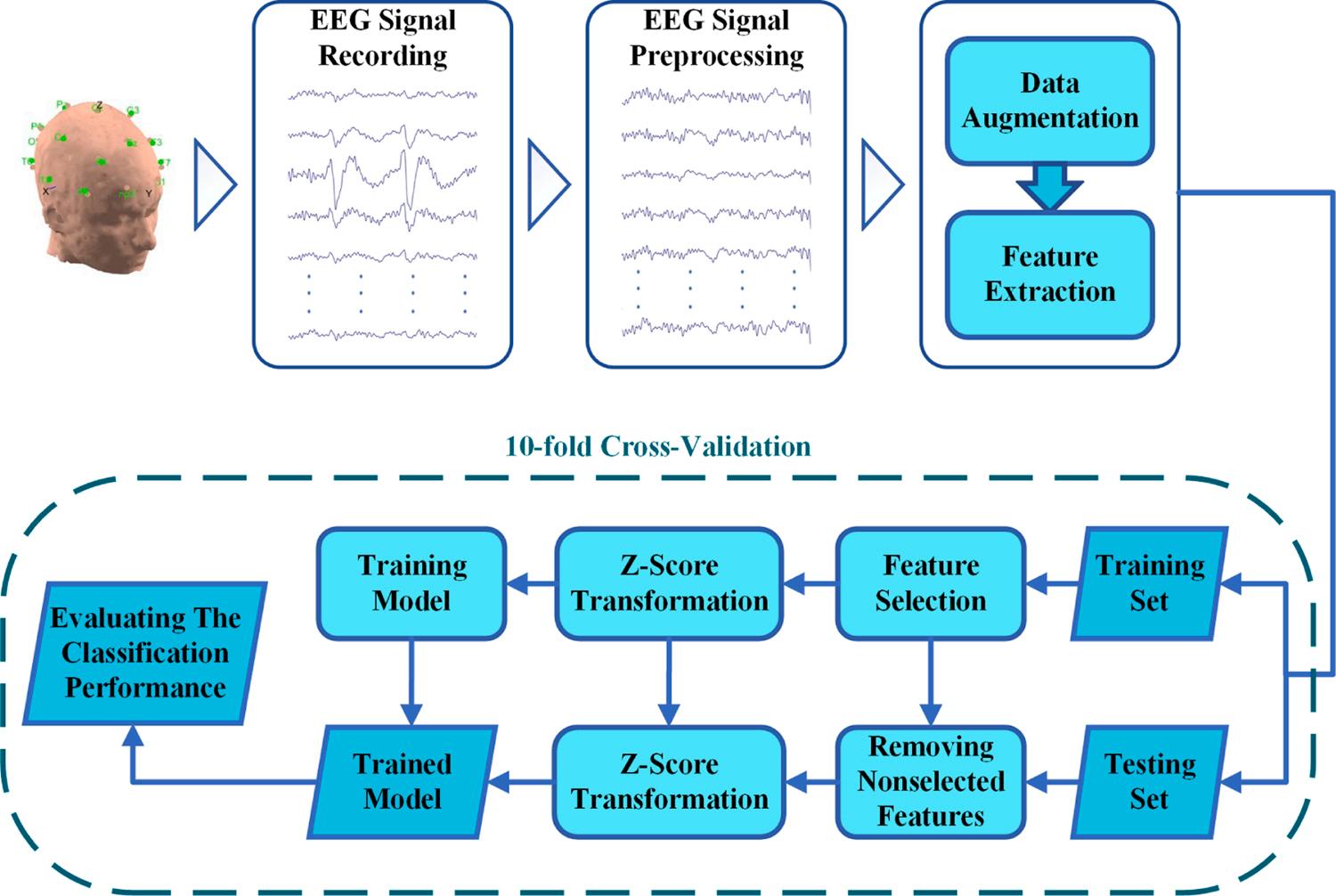
Fig. 1 illustrates the overview of the proposed framework for diagnosing MDD based on EEG signals. As shown in Fig. 1, the proposed method contains EEG signal preprocessing, data augmentation, feature extraction, feature selection, classification, and validation steps. In the first step, the typical noises and artifacts in the signals were suppressed
using the proposed preprocessing method. Next, the number of samples was increased using data augmentation procedure. In the feature extraction step, some measures based on statistical, spectral, wavelet, functional connectivity, and nonlinear analyses were extracted from each sample and arranged column-wise in a matrix called EEG feature matrix. As exhibited in Fig. 1, the feature matrix was then divided randomly into the training and testing sets using 10-fold crossvalidation. To improve the classification performance and reduce the dimensionality of the feature matrix, SBFS method was utilized as the feature selection technique. In this step, the training set was applied to the SBFS algorithm, so that it returned the best discriminative feature subset between HC and MDD classes. It is worth mentioning that SBFS returned a specific subset in each iteration of the execution of the proposed method using 10-fold cross-validation. Next, the classification model was trained and validated by the training and testing sets with selected features. Finally, the classification performance of the proposed method was evaluated based on the classification results of the testing set during each iteration. It should be mentioned that all simulations and implementations were conducted using MATLAB™R2019b on a system with Intel® Xeon® Processor E5-2697 v2 CPU at 2 GHz and 16 GB memory. More details of each step have been provided in the following.
2.3.1. EEG signal preprocessing
During recording, EEG signals get inherently contaminated with different types of noises and artifacts. The origins of these artifacts are various biological and non-biological sources such as eye blinks and movements, muscular activities, heartbeat, channel noise, and power line noise. As a result, EEG signals might not truly represent the underlying neuronal activity. Therefore, EEG signal preprocessing step is considered necessary for noise reduction and destructive artifacts suppression to ensure that preprocessed signals represent pure brainwave activity and avoid subsequent erroneous analysis.
In the present study, a proposed EEG signal preprocessing pipeline was employed, implemented using the EEGLAB toolbox (Delorme and Makeig, 2004) of MATLAB software. Firstly, each EEG signal was re-referenced to the A1-A2 channel. Next, all re-referenced EEG signals were high-pass filtered with 0.5 Hz cutoff frequency and low-pass filtered with 32 Hz cutoff frequency. This procedure suppresses muscle activity and power line noise since most of these artifacts’ power is
Fig. 1. Overview of the proposed framework for MDD diagnosis using 19-channel EEG signals.
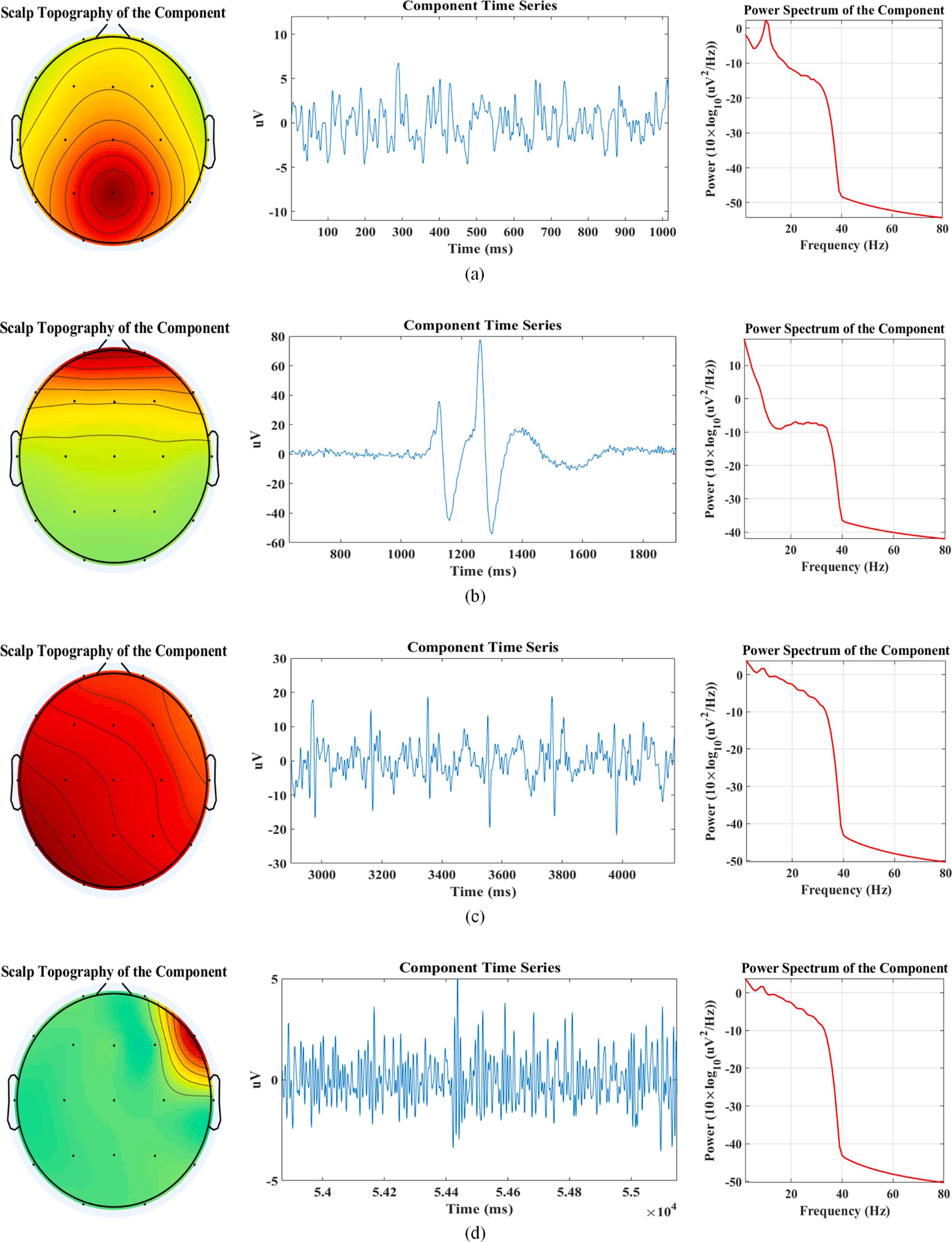
concentrated in higher frequencies. To remove other artifacts, independent components of filtered signals were calculated using the independent component analysis (ICA) algorithm. Since this method assumes that the EEG signal is a mixture of independent components, it decomposes the signal into these parts so that each part could belong to the cerebral and artifactual sources. After applying ICA on a signal, each component was identified as an artifact or cerebral component using a voting classification process with the aid of ICLabel (Pion-Tonachini et al., 2019) and MARA (Winkler et al., 2011) plugins and manual inspection of the component in time and frequency domains. In the voting classification process, each automatic plugin and the manual inspection method made a prediction (vote) for each component, and the final output prediction was the one that received more than half of the votes. Then, artifact components were removed, and the pruned signal was reconstructed. Fig. 2 illustrates the scalp topography, time-series, and power spectrum of some instances of the obtained independent components of the used dataset, which belong to the brain, eye blinking, heartbeat, and muscular activities. Finally, the pruned EEG signal was visually inspected in the time domain to eliminate the remaining noisy intervals.
2.3.2. Data
augmentation
In machine learning applications, data augmentation is used to increase the number of samples without collecting new samples. A typical time-series data augmentation is based on the signal-slicing, which segments a signal into the smaller slices of equal lengths and the same labels, with the original EEG signal label. In this study, an EEG sample was segmented into slices with 1-min lengths to generate new samples and increase the dataset’s diversity. It is worth mentioning that 1-min slicing led to the better results for the proposed method compared with other slicing times. After performing data augmentation, an EEG dataset of HC and MDD subjects with more samples was obtained, consisting of 249 MDD and 261 HC samples, so that each sample included 19 channels. The reasons for the increase of HC samples than MDD cases after data augmentation were the different duration time of the dataset’s EEG signals, eliminating noisy intervals, and unavailability of some EEG signals.
2.3.3. Feature extraction
Feature extraction aims to derive meaningful parameters from a dataset providing informative features, reducing the number of variables, and facilitating the subsequent steps of machine learning frameworks. In this study, the feature extraction step involved statistical, spectral, wavelet, functional connectivity, and nonlinear analysis methods. This step constructed a feature matrix called EEG feature matrix consisting of 510 rows and 735 columns, where each row and each column represent each sample and its corresponding features, respectively. In the following, each category of the proposed features for classifying MDD and HC signals is described in detail.
(1) Statistical analysis: In this study, some statistical measures were extracted from artifact-free EEG segments as statistical features. The statistical features include average, skewness, kurtosis, minimum, maximum, and Hjorth parameters extracted from each channel of EEG segments. The Hjorth parameters proposed by Hjorth (1970) consist of three main measures called activity(h0 ), mobility(h1 ), and complexity(h2 ), which are defined as follows:
where x(t ) is the time-series, var is the variance function and x ′ (t ) is the first-order derivative of x(t ). The activity parameter represents the variance of a time-series signal. The mobility and complexity parameters indicate the proportion of the standard deviation of the power spectrum and the change in frequency of the signal, respectively.
(2) Spectral analysis: EEG spectral analysis intends to interpret the power of fluctuations of the EEG time-series in EEG frequency bands at different scalp regions. Numerous studies indicated the significant relationships between the characteristics of EEG spectral features and neurological disorders, cognitive state, and mental illnesses. Therefore, EEG spectral features may be useful for characterizing EEG signals to be recognized and analyzing cognitive states or neurological dysfunctions. The proposed method employed the band power of EEG signals in the typical EEG frequency bands and interhemispheric asymmetry as EEG spectral features. These frequency bands are associated with different cognitive tasks, mental states, and neurological brain mechanisms, and could be interpreted as depression biomarkers because of their relation with various mental states. For instance, beta frequency band is associated with expectancy, consciousness, memory, and problem-solving, and having too much of that may lead to excessive stress and anxiety (Freeman and Quiroga, 2012; Abhang et al., 2016; Evans and Abarbanel, 1999). Alpha frequency band is related to relaxation state, and prominence of that causes daydreaming, inability to focus, and deep relaxation. In contrast, its suppression can lead to anxiety, high stress, and insomnia (Abhang et al., 2016; Evans and Abarbanel, 1999; Rao, 2013). Theta frequency band is involved in shallow sleep state, emotional processing, creativity, memory, and perceptual functions. The unbalanced of this activity may result in anxiety, poor emotional awareness, stress, hyperactivity, and impulsivity (Abhang et al., 2016; Evans and Abarbanel, 1999; Rao, 2013; Li et al., 2019; Aftanas et al., 2002). Delta frequency band is typically associated with the deepest levels of relaxation and restorative and healing sleep. If delta activity is abnormal, a person may experience learning impairment, inability to think, or difficulties maintaining conscious awareness (Freeman and Quiroga, 2012; Abhang et al., 2016; Evans and Abarbanel, 1999; Harmony et al., 1996; Knyazev, 2012). Furthermore, many studies have shown relationships between EEG frequency bands and MDD with different results. For example, it was observed that the decreased theta and delta activity are related to MDD (Saletu et al., 2010; Knott et al., 2001; Coutin-Churchman and Moreno, 2008). In contrast, it was reported that increased delta and theta activity was associated with MDD (Liu et al., 2017; Nystrom et al., 1986). Some studies determined relations between MDD and variation of alpha and beta activity (Coutin-Churchman and Moreno, 2008; Lee et al., 2018; Roh et al., 2016; Begi´ c et al., 2011). Although many studies have been conducted about the relation between MDD and EEG frequency bands, a consistent finding has not been obtained due to methodological differences across studies and the inherent heterogeneity of the populations under investigation. Herein, the power of four common EEG frequency bands, i.e., delta (0.5–4 Hz), theta (4–8 Hz), alpha (8–13 Hz), and beta (13–32 Hz) were computed. To compute the power of frequency bands, the Welch periodogram method was used to estimate the power spectral density of signals (Oppenheim et al., 1989). In this work, the Hamming window with 50% overlap between the segments was used to estimate the Welch power spectral density. Interhemispheric asymmetry is a spectral feature that measures EEG signal power differences between the left and right hemispheres in the common EEG frequency bands (Hinrikus et al., 2009). The equation of interhemispheric asymmetry can be modeled as follows:
R.A. Movahed et
2. The scalp topography, time-series, and power spectrum of some instances of the obtained independent components of the EEG dataset signals. (a): Brain component, (b): eye blinking component, (c): heart activity component, (d): muscular activity component.
Fig.
Amn = log(PRH ) log(PLH ), (4)
where Amn , PRH , and PLH are the interhemispheric asymmetry, the power of EEG signal in the right hemisphere, and the power of EEG signal in the left hemisphere, respectively. Here, the interhemispheric asymmetry was computed for delta, theta, alpha, and beta frequency bands for each EEG channel pair. The channel pairs in this study were Fp2-Fp1; F4-F3; F8-F7; C4-C3; T4-T3; P4-P3; T6-T5; O2O1.
(3) Wavelet analysis: Wavelet transform is a time-frequency decomposition technique that provides better time-frequency localization than other similar methods such as empirical mode decomposition and short-time Fourier transform (Rosso et al., 2006). It utilizes time windows with different lengths, decomposing a signal into different frequency resolutions. The continuous wavelet transform (CWT) of a time-series signal is defined as follows:
where i = 1, 2, , N indicates the level of the wavelet decomposition.
(4) Nonlinear analysis: EEG signals are non-stationary and stochastic, inherently, containing some nonlinear characteristics. These properties limit the linear analysis to describe these signals completely. Therefore, many studies related to EEG signal processing employ nonlinear analysis to investigate the complexity and dynamics of these signals. In this study, some nonlinear methods such as detrended fluctuation analysis, Higuchi, correlation dimension, Lyapunov exponent, C0-complexity, Kolmogorov entropy, Shannon entropy, and approximate entropy were applied to the preprocessed EEG segments to extract nonlinear features.
where x(t ) is the time-series signal, ψ is the shifted and scaled wavelet basis, and a and b are the scaling and shifting parameters, respectively. Unfortunately, the information obtained by CWT may be highly redundant and requires a high computation load to be achieved. The discrete wavelet transform (DWT) is proposed to address this problem, which is defined as follows: DWT(a, b) = 1
where j and k represent the frequency and time localization, respectively. In the optimum DWT, the signal is passed through quadrature mirror filters, consisting of a series of high-pass and lowpass filter pairs. These filter pairs decompose a signal into the approximate (Ai ) and detail (Di ) coefficients, which represent low and high-frequency components of the signal, respectively. This decomposing procedure can be applied to the Ai coefficients for several times, creating a hierarchal structure. In this research, the three-level DWT decomposition was conducted by Coiflet 5 window function.
After that, RWE and WE were computed as wavelet features using wavelet coefficients. The energy at the kth decomposition level (Ek ) can be obtained using (7), which is defined as follows: Ek = ∑ l ⃒ ⃒Ck l ⃒ ⃒ 2 , (7)
where Ck,l is the wavelet coefficients at the kth decomposition level, l is the number of coefficients, and k = 1, 2, , N denotes the decomposition level. The total energy (ET ) at the kth decomposition level is obtained using (8), formulated as follows: ET = ∑ N
Then, RWE at kth resolution level (RWEk ) can be computed using the following equation:
RWEk = Ek ET (9)
The equation of WE is based on Shannon entropy formulation, which is represented as follows:
(11) Detrended fluctuation analysis: Detrended fluctuation analysis is a mathematical approach for analyzing stochastic processes that estimates the correlation properties of a timeseries signal (Jospin et al., 2007). In the first step of this analysis, given a finite time-series signal, x(t ) of length N, the summation of it (X(k)), is computed using the following equation:
where x denotes the average value of x(t ) Then, X (k) is divided into the n time windows with equal lengths, and a least-squares line was fitted to the data within each window. Let Yn (k) indicate the resulting least-squares line fitting. Next, the fluctuation (F (n)) is computed using the following equation:
Finally, the calculation process of (12) is repeated for time windows with different sizes to construct a logarithmic scale of F (n) against n The relation between logarithm of F (n) and n can be expressed by F (n) = nα , which α represents the correlation properties of the time-series signal.
(12) Higuchi: In 1988, Higuchi introduced a method for estimating the fractal dimension of a set of points (Higuchi, 1988). Suppose x(t ) is a time-series signal with a length of N samples. Given this signal, T new time-series signals are generated using (13),
where τ = 1, 2, …, T and [r] is the integer part of r. The length of each time-series (Lτ (T )) is defined as follows:
In this algorithm, an average length is calculated for each timeseries using the below equation:
WE = ∑ N i=1 RWEk logRWEk , (10)
The calculation of (15) is replicated for all T values ranging from Tmin to Tmax . Finally, the slope of the linear fitting of lnL(T ) versus ln 1/T is estimated as the fractal dimension of x(t ). In this research, the Tmin and Tmax were chosen to 1 and 30 values, respectively.
(13) Correlation dimension: Correlation dimension is a method for estimating the space’s dimensionality occupied by a set of random points. Grassberger and Procacia proposed the most commonly used correlation dimension algorithm in 1983 (Grassberger and Procaccia, 2004). In the first step, this algorithm generates an m-dimensional vector using time delay (τ) and embedding dimension (m), which can be represented as:
X (i) = [x(i), x(i + τ ), , x(i + (m 1)τ ) ], (16)
where i = 1, 2, , N (m 1)τ, x is the time-series signal with N samples, and X is the m-dimensional vector. After that, the correlation integral of X is computed using the following equation: C (r ) = 2
where C(r) is the correlation integral and ϕ is the Heaviside step function. Next, the raw correlation dimension is estimated using (18), which is denoted as follows:
D = lim r→0 lnC (r ) ln(r ) (18)
The computation of (18) is repeated by increasing m, resulting in a gradual increase of D until it is saturated. The saturated value of D is the estimated correlation dimension of x(t ) signal. (14) Lyapunov exponent: Lyapunov exponent is a measure of dynamic systems that characterizes the rate of convergence or divergence of close trajectories in phase space (Roschke et al., 1995). For a dynamic system with d dimension, d number of Lyapunov exponents can be computed. However, the largest Lyapunov exponent (LLE) is calculated instead of all exponents in most practical applications. For a dynamical system, the maximum Lyapunov exponent (λ1 ) can be defined as follows:
dj (i) = dj (0)exp(λ1 i▵t ), (19)
where dj (i) is the average Euclidian distance between two neighbor trajectories at i time and dj (0) is the Euclidian distance between the jth pair of initially most adjacent neighbors after i time. The LLE is calculated using (20), which is defined as follows:
y(i) = 1 ▵t < ln( dj (i) ) >, (20)
where y(i) is the approximated LLE and < ln( dj (i) ) > is the mean value of the natural logarithm of dj (i) over all values of j. (15) C0-complexity: C0-complexity is a measure to quantify irregularities in a time-series signal proposed by Shen et al. (En-hua et al., 2005). In summary, a time-series signal can be divided into the regular and stochastic components, and the C0-complexity defines the proportion of the amount of irregularity to the regularity of a signal. In other words, it indicates the complexity and randomness of a time-series.
Given a time-series signal x(n) with N samples, the mean amplitude of the power spectrum of x(n) (M) can be obtained using (21): M = 1 N ∑ N 1 k 0 |X (k ) |2 , (21)
where X(k) is the fast Fourier transform of the x(n) A new spectrum is constructed using X (k) and M as follows:
Y (k ) = { X (k ) |X (k ) |2 > M 0 |
By calculating the inverse Fourier transform of Y (k) (y(n)), the C0complexity (C0) of the x(n) can be computed as follows:
where A1 and A0 are the power of irregular and regular parts of x(n), respectively.
(16) Kolmogorov entropy: Kolmogorov entropy (KE) is another measure for characterizing the chaotic degree of a system (Aftanas et al., 1997). It also reflects the rate of loss of information per unit of time for a time-series signal. Mathematically, it is defined based on the average rate of loss of information of a signal with n samples as follows:
where Pi0 in 1 is the loss of information per each sample. The positive and finite value of KE indicates that the dynamic phenomena in the time-series are chaotic. The zero value of this parameter means that the time-series contains regular phenomena, and infinite KE refers to the existence of non-deterministic phenomena in the signal.
(17) Shannon entropy: Shannon entropy is a quantity to measure the rate of the uncertainty of a random time-series, introduced by Shannon (Shannon, 1948). The larger value of this measure indicates more uncertainty and randomness of a signal. The Shannon entropy of a random time-series with N samples can be defined as:
where H and pi are the Shannon entropy of the signal and the probability of i sample in the time-series, respectively.
(18) Approximate entropy: In 1991, Pincus et al. proposed approximate entropy as an algorithm to quantify the rate of the unpredictability of a time-series signal (Pincus, 1991). The more value of approximate entropy shows the more irregularity of a time-series. Firstly, given a time-series x(n) with N data points, a new vector X(i) is constructed using (16) on the assumption that τ = 1. Next, the distance between X(i) and X (j) (D[X(i)), X(j) ]) is calculated as follows: D[X (i), X (j) ] = maxk=1,2, ,m [|x(i + k 1) x(j + k 1) | ] (26)
where | | is the Euclidean distance. After that, Cm i (r ) is computed for each i, i = 1, 2, , N m as follows:
R.A. Movahed
Cm i (r ) = numberof D[X (i), X (j) ] ≤ r N m 1 , (27)
where r is the threshold for D[X(i), X(j) ] Finally, the approximate entropy (ApEn) is defined as follows:
where the equation of Φm (r ) is:
m (r ) = 1
In this research, the values of m and r were chosen to 2 and 0 2var(x), respectively.
(5) Functional connectivity analysis: Different perceptual and cognitive tasks require a coordinated flow of information distributed in the brain regions. Functional connectivity is a method for analyzing the dynamic coordination of neuronal activities in the brain. In other words, functional connectivity investigates the statistical relationships between neurobiological activities and connections between different brain regions such as frontal, temporal, central, parietal, and occipital (Squire et al., 2009). Since some MDD-related cognitive tasks such as emotional regulation, thinking, attention, problem-solving, and memory-related functions are associated with frontal and temporal lobes and their connection, functional connectivity features could be interpreted as MDD biomarkers using brain network representation (Smith and Kosslyn, 2007; Uttal, 2011). Many studies have also shown that the pathogenesis of MDD is related to the abnormalities in the structures and networks of the brain regions (Zhu et al., 2012; Wu et al., 2013; Avery et al., 2014; Sheline, 2003; Koolschijn et al., 2009; Olbrich et al., 2014; Leuchter et al., 2012). Therefore, functional connectivity features could be effective for MDD diagnosis. There are different metrics for quantifying functional connectivity, such as coherence, mutual information, and synchronization likelihood. In this study, the synchronization likelihood metric was used to extract a set of features based on the functional connectivity analysis. Synchronization likelihood characterizes synchronization between two times-series signal (Stam and Van Dijk, 2002). The value of synchronization likelihood between two time-series ranges from [0,1] interval. The zero value represents the complete non-synchronization, while one value expresses the complete synchronization between two signals. Consider M simultaneously recorded EEG channels (xk,i ), where kε{1, 2, , M} and iε{1, 2, , N} denote the channel number and the index of each discrete sample, respectively. According to (30), an embedded vector (Xk,i ) is constructed using the EEG signal corresponding to a channel as follows:
Xk,i = [xk,i , xk,i+l , , xk,i +(m 1)l ], (30)
are used for autocorrelation effects and sharpen the synchronization measure’s time resolution. These parameters are chosen such that ω1 ≪ω2 ≪N. Next, the critical distance (εk,i ) is computed for each k and each i for which Pεk i k,i = pref , where pref ≪1. Now, the number of channels where the Xk,i and Xk,j will be closer together than εk,i (Hi,j ), is determined for each sample pair (i, j) and within the considered window (ω1 < |i j| < ω2 ) as follows:
Hi,j = ∑ M k 1 ϕ( εk,i ⃒ ⃒Xk ,i Xk,j ⃒ ⃒ ) (32)
In other words, Hi,j indicates how many of the embedded signals resemble each other. In the next step, the synchronization likelihood for each channel (k) and each discrete sample pair (i, j), (Sk,i,j ) is defined as follows:
Hi,j 1
,i,j =
Finally, the synchronization likelihood (Sk,i ) is computed as follows:
Sk,i describes the rate of synchronization between channel k at sample i and other M 1 channels. If Sk,i = pref , all M signal channels are uncorrelated whereas Sk,i = 1 indicates the maximum synchronization of all M signal channels. In this study, the pref , l, m, the size of ω1 and ω2 were chosen to 0.01, 10, 10, 100, and 410, respectively. It is worth mentioning that the synchronization likelihood between the same channels was removed, and the synchronization likelihood between different channels has remained as the functional connectivity features.
2.3.4.
Feature selection
In machine learning or statistical pattern recognition applications, the extracted features from a dataset may contain redundant or irrelevant features. In another point of view, high-dimensional extracted features increase the computational load, which leads to the overfitting issue of the models. Feature selection is a technique to select the desired subset of features, reduce the dimension of feature space, and improve the classification performance of the pattern recognition model. In this work, SBFS was utilized to select a subset of features for improving the classification performance. The steps of this algorithm are summarized in Algorithm 1. In this study, the objective criterion (J) was defined as the mean of misclassification rates during 10-fold cross-validation process. This algorithm initially considers the whole feature set and then sequentially removes features from the feature set until the elimination of further features leads to the increase of the objective criterion (Pudil et al., 1994). It should be mentioned that the classifier model in the SBFS step is the same as the classifier model in the classification step of the proposed method.
Algorithm 1 The SBFS algorithm
Input: The set of all features, Y = {y1 , y2 , , yd }
(31)
where m and l are the embedding dimension and lag parameters, respectively. To estimate that the embedded vectors are closer to each other than a distance of ε, a probability distribution (Pε k,i ) is considered for each channel (k) and each sample (i). The formulation of Pε k,i is defined as follows: Pε k,i = 1 2(
where ϕ, | |, ω1 ,and ω2 are Heaviside step function, Euclidean distance, Theiler correction window,and sharpening window, respectively. The Theiler correction window and sharpening window
Output: An optimum subset of features, Sk = {Sj |j = 1, 2, , k; Sj εY} where k = 1, 2, , d
1. Start with the full set, S0 = Y
2. Remove the worst feature, s∗ = argmax(J(Sk s) ), where s ε Y Sk
3. Update Sk+1 = Sk s∗ ; k = k + 1.
4. If J(Sk ) > J(Sk 1 ), go to step 6.
5. Else go to the step 2. 6. Stop.
2.3.5. Classification
Classification is a fundamental part of the automatic identification of patterns in many statistical pattern recognition problems. In the present study, different classifiers such as Support Vector Machine with linear (LINSVM) and radial basis function (RBFSVM) kernels, LR, DT, NB, and some ensemble classifiers like RusBoost (RB), GentleBoost (GB), and Random Forest (RF) were employed to select the best one for the proposed machine learning framework. A data standardization based on zscore transformation was performed on the training and testing sets to modify unequal distribution of each feature and eliminate outliers. It should be mentioned that the hyperparameters of LINSVM, RBFSVM, LR, DT, NB, RB, and GB classification models were optimized using the Bayesian optimizer. It is worth mentioning that the number of trees in the RF ensemble classifier ranged from 2 to 50 during the training procedure to find the optimum value of this hyperparameter.
2.3.6. Validation
In the present study, 10-fold cross-validation was employed to fairly assess the classification performance of the proposed method. In this procedure, the dataset is initially divided into 10 folds, of which 9 folds are randomly used as a training set, and the remaining fold is employed as a testing set. This process is repeated 10 times until each fold is utilized as a testing set. During each iteration, the testing set is applied to the trained model, which results in 10 different evaluation metrics values. For investigating the overall classification performance, the average and the standard deviation of the evaluation metrics were considered. The evaluation metrics used in this study were accuracy (AC), sensitivity (SE), specificity (SP), F1-score (F1), and false discovery rate (FDR), which are defined as follows:
and investigated. Finally, the proposed method was evaluated using another independent dataset, and its results were reported in the last part of this section.
3.1. Results per classifier models
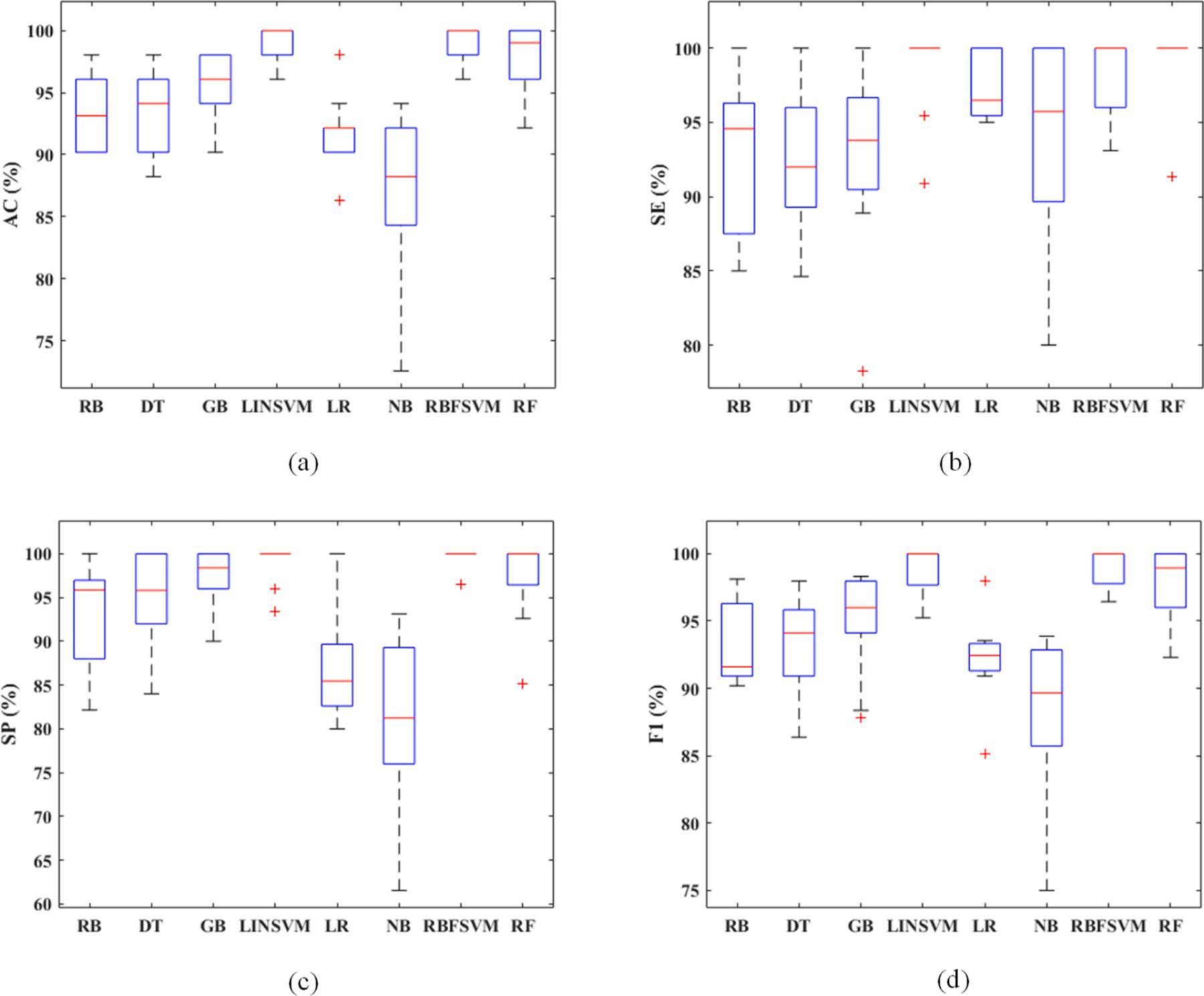
Table 1 shows the numerical results of the proposed method using different classifier models. As demonstrated, RBFSVM classifier model provided the best performance among all classifiers with the highest mean of AC, SP, and F1 metrics and the lowest mean of FDR measure. The average AC, SE, SP, F1, and FDR metrics obtained by RBFSVM classifier were 99.0%, 98.4%, 99.6%, 98.9%, and 0.4%, respectively. RBFSVM classifier obtained the lowest standard deviation of AC, SP, F1, and FDR metrics compared to the other utilized classifiers, which indicates the more robustness of this classifier’s performance in the proposed method. According to the reported results in Table 1, the second and third best classifiers in the proposed method were LINSVM and RF classifiers, respectively. NB classifier exhibited the worst performance with the lowest mean of AC, SP, and F1 metrics. The other classifiers provided a similar performance. Overall, the obtained results show that all of the utilized classifiers except NB classifier approximately achieved reliable and accurate performances for the classification of MDD and HC cases. Fig. 3 illustrates the box plots of the obtained values of AC, SE, SP, and F1 metrics using different classifiers. As shown in Fig. 3, the obtained AC, SE, SP, and F1 metric values of all classifiers except NB classifier were relatively high, which confirms the acceptable performance of the proposed method. However, the AC, SE, SP, and F1 metric values of RBFSVM classifier were higher than the computed values of these metrics using other classifiers. Also, the boxplots of the AC, SE, SP, and F1 metrics of RBFSVM and LINSVM classifiers had the lowest height compared to the other classifiers, indicating that the performance metric values of RBFSVM and LINSVM classifiers were closer to the average performance compared to the other methods. Therefore, it can be proven that RBFSVM and LINSVM classifiers provided the optimal robustness/performance compared to the other classification models for the proposed classification framework.
3.2. The effect of data augmentation
where TP is the number of MDD samples that are correctly classified, FN is the number of MDD samples that are incorrectly classified as HC samples, FP is the number of HC samples that are incorrectly classified as MDD cases, and TN is the number of HC cases that are correctly classified.
3. Results
In this section, the performance of the proposed machine learning method to diagnose MDD based on EEG signals is evaluated in several aspects. In the first part, the obtained numerical results of various classifiers in the proposed framework are provided. In the second part, the effect of the data augmentation procedure on the proposed framework is analyzed. Next, the obtained results of the proposed method are compared with the previous approaches. Then, each set of features is individually used as a feature matrix to assess their performance for classifying MDD and HC signals. In the fifth part, the EEG signal power differences between MDD and HC subjects are investigated. The most significant functional connectivity features are analyzed in the sixth part of this section. Next, the intersection of the returned subsets by SBFS in 10-fold cross-validation execution of the proposed method is reported
In order to analyze the effect of data augmentation on the performance of the proposed method, EEG signals with different segment lengths were applied to the proposed classification framework. Firstly, the proposed framework was validated without data augmentation. Then, it was tested by 1- and 2-min EEG segments. The obtained results of these simulations based on the three best classifiers are reported in Table 2 As shown in Table 2, the proposed method with both data augmentation strategies, 1- and 2-min slicing, achieved a better classification performance. In other words, the presented framework with both data augmentation strategies achieved higher means of AC, SE, SP, F1 metrics, and lower means of FDR measure compared to the proposed method without data augmentation. Only 2-min slicing with RBFSVM classifier led to a higher FDR mean than the 1-min and without slicing conditions. According to the results, it can be interpreted that the data augmentation procedure with 1-min slicing led to the best classification performance.
3.3.
Comparison with other methods
In order to compare the performance of the proposed method with other approaches, we implemented the methods described in (Mahato and Paul, 2020; Mahato and Paul, 2019; Mumtaz et al., 2017; Mumtaz et al., 2018; Mumtaz et al., 2017). For a fair comparison, all of the methods were validated using 10-fold cross-validation technique. It is worth mentioning that the generated indices for training and testing sets using 10-fold cross-validation were considered the same for all approaches. Table 3 provides the obtained numerical results of the
R.A. Movahed
Table 1
The classification results of the proposed method using different classifier models in terms of the percentage (%) of the mean and
deviation of AC, SE, SP, F1, and FDR metrics.
proposed method as well as the previous ones for automatic diagnosis of MDD based on EEG signals. According to the summarized results in Table 3, the proposed framework achieved the highest mean of AC, SE, SP, and F1 metrics and the lowest mean of the FDR metric compared to the other methods, indicating that the proposed method is more accurate for the classification of MDD and HC subjects based on EEG signals. In another point of view, the proposed method, compared with (Mumtaz et al., 2018; Mahato and Paul, 2020; Mahato and Paul, 2019; Mumtaz et al., 2017; Mumtaz et al., 2017), improved the AC mean by 7.60%, 19.56%, 17.85%, 15.78%, and 28.73%, respectively. Furthermore, the proposed method achieved the lowest standard deviation between all evaluation metrics compared to the previous approaches of the automatic classification of MDD and HC subjects based on EEG signals.
Compared to (Mumtaz et al., 2018; Mahato and Paul, 2020; Mahato and Paul, 2019; Mumtaz et al., 2017; Mumtaz et al., 2017), it has been observed that the AC standard deviations were reduced by 68.29%, 80.59%, 87.25%, 81.42%, and 84.88%, respectively using the proposed method. These results demonstrate that the classification performance of the proposed method is relatively stable and more reliable than other methods.
3.4. Results per feature set
In this section, each set of the proposed features was used as the feature matrix individually in the proposed method using RBFSVM, LINSVM, and RF classification models. Table 4 lists the classification
Fig. 3. The box plots of the achieved values of AC (a), SE (b), SP (c), and F1 (d) metrics per each classifier using 10-fold cross-validation method.
Table 2
The comparison of the classification results of the proposed method using data augmentation procedure with 1- and 2-min slicing and without data augmentation, in terms of the percentage (%) of the mean and standard deviation of AC, SE, SP, F1, and FDR metrics. Method
1-min slicing
2-min slicing
Table 3
The comparison of the classification results between the proposed method and previous works for identifying MDD and HC subjects based on the EEG signals. Method
and Paul, 2020)
et al.,
et al., 2017)
Table 4
The classification results of the proposed method based on RBFSVM, LINSVM and, RF classification models using
(%) of the mean and standard deviation of AC, SE, SP, F1, and FDR metrics.
Functional connectivity
results based on each feature set and integrated feature sets using the mentioned classifiers.
It is clear from the provided results in Table 4 that the integrated EEG feature sets achieved a better performance than each EEG feature set. By
comparing the results, it can be concluded that the integrated feature sets obtained the highest average of AC, SE, SP, and F1 parameters and the lowest mean of the FDR metric. In addition, the integrated feature sets provided the classification results with the lowest standard
deviation of evaluation metrics. It is worth mentioning that the best classification performance of the integrated feature sets was obtained by RBFSVM classifier, which provided a classification performance with an average AC of 99.0%, SE of 98.4%, SP of 99.6%, F1 of 98.9%, and FDR of 0.4%.
As demonstrated in Table 4, the functional connectivity feature set achieved the highest classification accuracy compared to the other EEG feature sets. In other words, it obtained the highest mean of AC, SE, and F1 measures among all EEG feature sets. These results show the superiority of the functional connectivity feature set compared to the other feature sets for the automatic classification of MDD and HC subjects based on EEG signals. For this feature set, RBFSVM classifier provided the best classification performance with an average AC of 93.3%, SE of 93.9%, SP of 92.8%, F1 of 93.2%, and FDR of 7.3%.
According to Table 4, the second best feature set for the automatic classification of MDD and HC subjects based on EEG signals was the spectral feature set. By comparing the functional connectivity and spectral feature sets results, the spectral feature set was determined to obtain the higher means of SP metric and lower means of FDR measure. It indicated that this feature set is more accurate to classify HC samples. For this feature set, RBFSVM classification model obtained the best classification performance by providing an average AC of 92.5%, SE of 91.9%, SP of 93.2%, F1 of 92.6%, and FDR of 6.5%.
According to the reported results in Table 4, the third best feature set in terms of classification performance was the nonlinear feature set, and its best performance was achieved by RBFSVM classifier (AC=87.4%, SE=87.3%, SP=87.8%, F1=86.9%, and FDR=13.1%).
Among these feature sets, the statistical and wavelet feature sets obtained the worst classification performance, respectively. For the statistical feature set, LINSVM and RF classifiers performed almost identically and achieved the highest classification performance. The best classification results with the wavelet feature set were obtained by RF classification model (AC=85.8%, SE=81.2%, SP=90.5%, F1=84.5%, and FDR=10.9%). Therefore, it can be interpreted that the wavelet feature set obtained the worst classification performance compared to the other EEG feature sets.
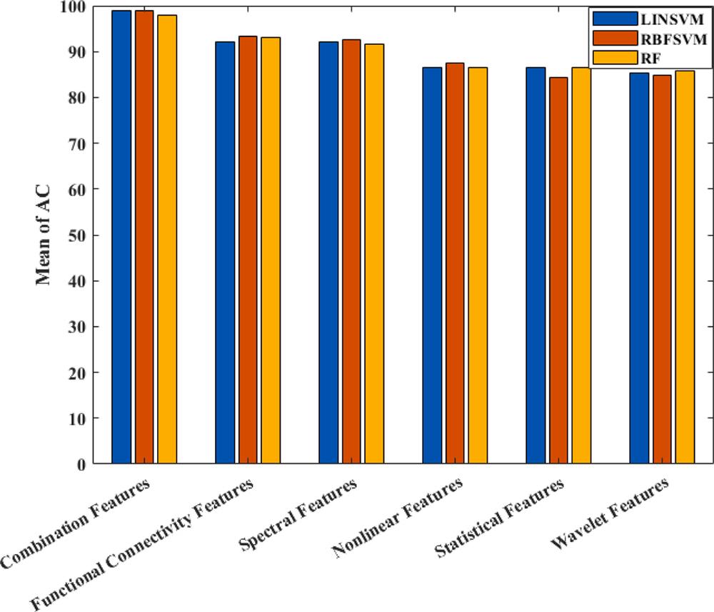
Fig. 4 exhibits the bar plot of the average accuracies achieved by each EEG feature set and the combination of them using LINSVM, RBFSVM, and RF classification models. As depicted in Fig. 4, the combination of all feature sets achieved the highest mean of AC metric (AC=99.0%). Among the feature sets, the functional connectivity
feature set obtained the highest mean of AC (AC=93.3%). The spectral, nonlinear, and statistical feature sets achieved the second, third, and fourth highest mean of AC, respectively. It is worth mentioning that the highest average of AC by spectral, nonlinear, and statistical feature sets were 92.5%, 87.4%, and 86.6%, respectively. The wavelet feature set achieved the lowest AC mean compared to the other EEG feature sets by providing the average AC of 85.8%.
3.5. EEG signal power analysis
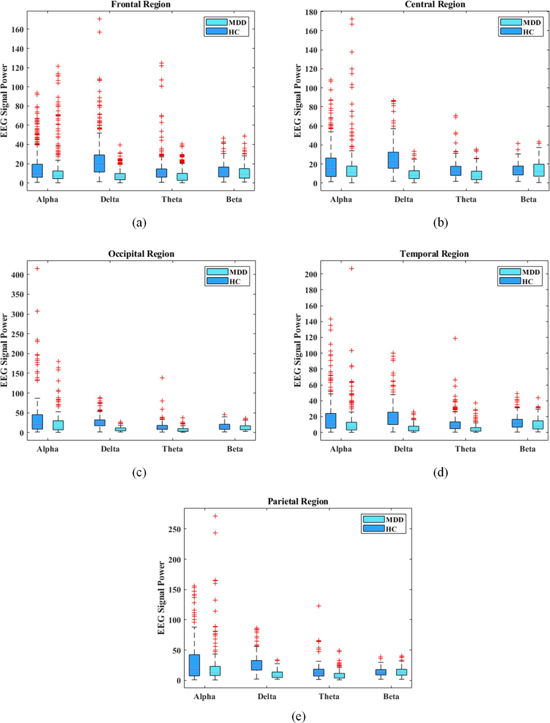
The main goal of this section is to investigate the EEG signal power differences in common EEG frequency bands at different scalp regions between MDD and HC samples. To this end, the alpha, theta, beta, and delta band powers of MDD and HC cases were analyzed by t-test and ftest methods to measure the difference between the two groups by the mentioned features. Table 5 lists the t-test and f-test results on the alpha, theta, beta, and delta EEG signal powers of MDD and HC cases in each channel. The delta power provided the most significant difference between MDD and HC samples in all brain regions based on the reported results. The second best EEG power for MDD and HC discrimination was the theta power. Nevertheless, the alpha and beta powers could not provide a significant difference between MDD and HC samples. However, the alpha power could provide more discrimination between MDD and HC samples compared to the beta power, especially in occipital and temporal regions. In terms of brain regions, the frontal, temporal, and parietal provided the most discrimination between HC and MDD samples using delta and theta powers. The best scalp regions for alpha power were temporal and occipital regions. It was also observed that the beta powers of the temporal region, especially on the right side, provided more discrimination than the beta powers of other brain regions. Fig. 5 illustrates the boxplots of alpha, theta, beta, and delta EEG signal powers of MDD and HC samples at the frontal, temporal, parietal, occipital, and central scalp regions. As demonstrated in Fig. 5, the most discriminative EEG signal powers between MDD and HC subjects in all regions were delta, theta, alpha, and beta powers, respectively. Fig. 5 shows that the delta power provided the most significant difference between the MDD and HC classes. It has been observed that the theta and alpha signal powers provided a slight difference between the MDD and HC samples. However, the theta signal power provided more discrimination between MDD and HC samples than the alpha signal power. Nonetheless, the beta signal power in all regions did not provide significant differences between the MDD and HC cases.
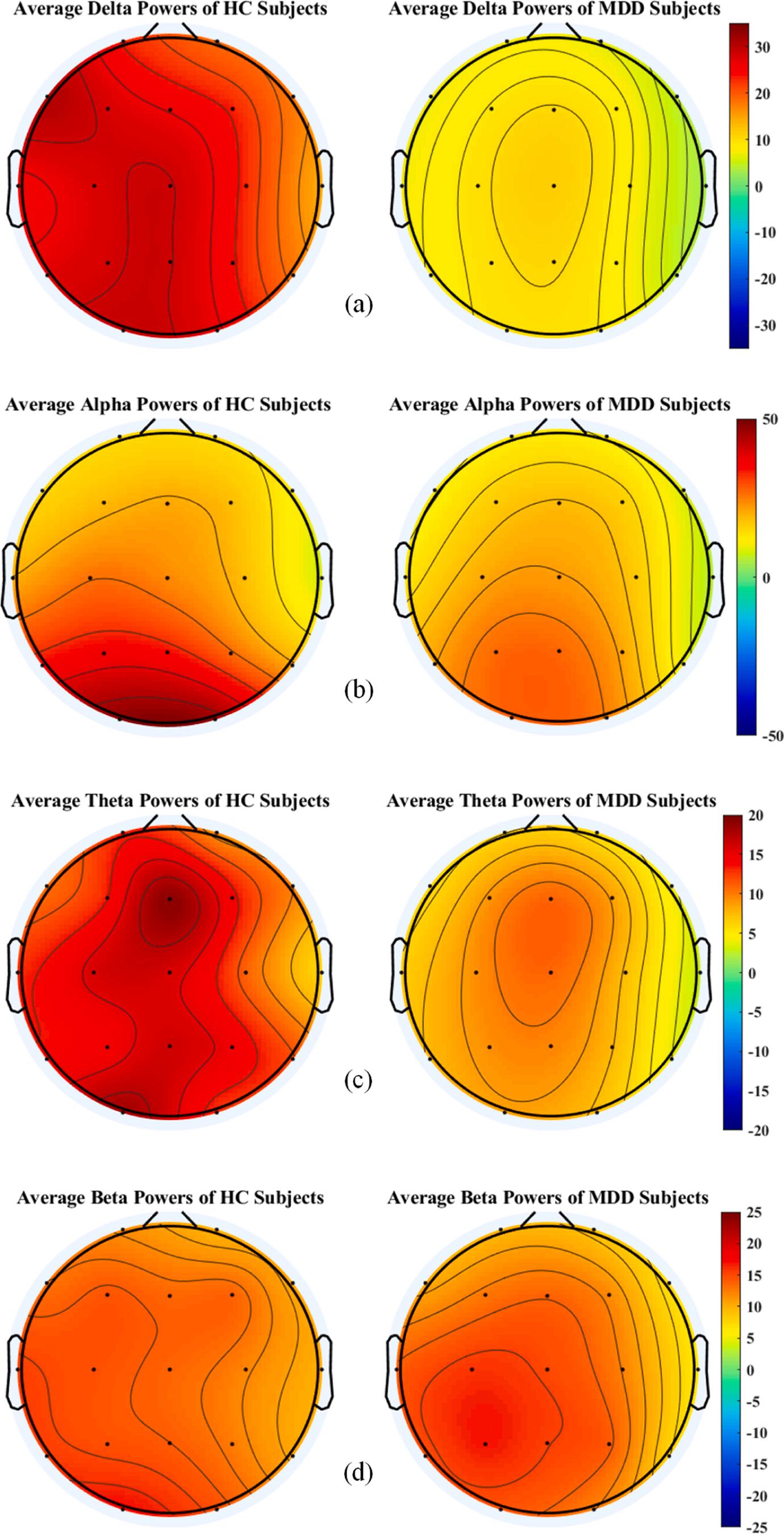
Fig. 6 shows the constructed scalp topographic maps of HC and MDD samples in terms of average powers of alpha, delta, beta, and theta frequency bands in each EEG channel. As depicted in Fig. 6, the delta power in all brain regions provided significant differences between HC and MDD cases. In addition, the theta power showed significant differences between HC and MDD cases, especially in temporal and frontal regions. In other words, it was observed that MDD cases had lower delta and theta activity compared to HC cases. Also, the MDD class had lower average alpha powers than the HC class in frontal, occipital, parietal, and central regions. In terms of beta power, the right temporal region provided more discrimination between HC and MDD cases than other regions. However, the beta power did not significantly differentiate HC and MDD cases in other scalp regions.
3.6. Functional connectivity analysis
According to the mentioned results, the best individual EEG-derived feature set for discrimination between HC and MDD cases is the functional connectivity feature set. In this subsection, the most significant functional connectivity features which discriminate HC and MDD cases are investigated. To this end, the functional connectivity features of MDD and HC cases were ranked using the p-value metric of t-test method, and ten top of them were determined. For more investigation, these ten top features were also analyzed by f-test method. Table 6
Fig. 4. the bar plot of the obtained AC metrics achieved by each EEG feature set and the combination of them using RBFSVM, LINSVM and, RF classification models. R.A. Movahed
Table 5
The t-test results on the alpha, theta, beta, and delta EEG band powers in each EEG channel. Bolded items indicate p value < 0 01.
Frontal
reports ten top significant functional connectivity features with their ttest and f-test results. Also, the boxplot of ten top significant functional connectivity features of MDD and HC cases is illustrated in Fig. 7 According to these results, the computed statistical significance of ten top functional connectivity features using t-test method for the difference between MDD and HC cases is less than 1e-6, which indicates the significant difference between the classes using each of these features. These ten top features were the F4-F8, T5-P4, T5-T6, Fz-Fp2, Fp1-Fz, T5T4, Fp1-Fp2, T5-C4, Fz-F8, and T5-Cz, which provided the most significant difference between HC and MDD cases among functional connectivity features. Additionally, the exhibited boxplots in Fig. 7 show that these ten top features can lead to significant differences between MDD and HC cases. Moreover, it can be interpreted that the functional connectivity between frontal and temporal scalp regions provided the most significant differences between MDD and HC classes.
3.7. Selected features
In the experimental setup of this study, SBFS method returns a specific subset of features as selected features in each iteration of 10-fold cross-validation execution, which resulted in 10 subsets of features for all iterations. In this subsection, the intersection of all these 10 subsets is reported and investigated. Table 7 lists these features with their details. The number of these features was 506, of which 108 belonged to the spectral set, 171 belonged to the functional connectivity set, 77 belonged to the statistical set, 54 belonged to the wavelet set, and 96 belonged to the nonlinear set. It was observed that all functional connectivity and spectral features were selected in all iterations and had the largest share in the selected features, while statistical and wavelet features had the least share in the selected features.
3.8.
Validation on independent dataset
In order to evaluate the proposed method on another independent dataset, we applied the MODMA EEG dataset of MDD and HC subjects (Cai et al., 2020) to the proposed method using 10-fold cross-validation.
This dataset contains 128-channel resting-state EEG signals acquired from 24 MDD patients and 29 HC subjects. It should be mentioned that the 19 EEG channels compatible with the proposed framework were extracted from each signal to prepare the mentioned dataset for validating the proposed framework. Table 8 reports the obtained results of this assessment using the three best classification models. As shown in Table 8, LINSVM provided the best classification performance by obtaining an average AC of 97.3%, SE of 98.3%, SP of 97.0%, F1 of 97.6%, and FDR of 2.5%. By comparing the results in Table 8 and the results of LINSVM, RBFSVM, and RF classifiers in Table 1, it can be interpreted that the obtained results by the proposed method were close in both cases, and it provided an acceptable and robust performance on both datasets.
4. Discussion
This study proposes an EEG-based machine learning framework to discriminate MDD and HC cases automatically. The proposed framework utilized various EEG-derived features such as statistical, spectral, wavelet, functional connectivity, and nonlinear features. In other words, the main objective of this study was to analyze the combination of different types of EEG-derived features to classify MDD and HC subjects. Also, different classification models were evaluated and compared to select the best one for the proposed framework. In order to select the best subset of features, SBFS algorithm was used. According to the reported results in Table 1, the best classification performance on the Mumtaz et al. (Mumtaz et al., 2017) EEG dataset, was provided by RBFSVM model by obtaining an average AC of 99%, SE of 98.4%, SP of 99.6%, F1 of 98.9%, and FDR of 0.4%. Also, the best classification performance on MODMA dataset (Cai et al., 2020) as the independent dataset, was provided by LINSVM model by providing an average AC of 97.3%, SE of 98.3%, SP of 97.0%, F1 of 97.6%, and FDR of 2.5%. These results on both datasets indicate the accurate and robust classification performance of the proposed framework. Furthermore, each set of EEG-derived features was individually evaluated in the proposed framework for discriminating the EEG signals of MDD and HC cases.
Although the obtained results confirm the high potential of all proposed EEG-based feature sets to distinguish MDD patients and HC subjects, the combination of all proposed EEG-based feature sets provided the best classification performance. Among the feature sets, the functional connectivity and spectral feature sets achieved the best performance, respectively. Another advantage of these feature sets is that they could also provide some biological information about MDD and some
MDD-related mental states and cognitive tasks. In addition, these feature sets had the largest share in the intersection of returned feature subsets by SBFS during 10-fold cross-validation and were selected in all iterations. It is worth mentioning that the wavelet feature set could obtain better results by changing its hyperparameters, such as window function, decomposition level, and combining the wavelet features of different decomposition levels. Besides, analyzing EEG signal powers of
Fig. 5. the boxplots of the delta, alpha, theta, and beta signal powers of MDD and HC subjects at frontal (a), central (b), occipital (c), temporal (d), and parietal (e) areas of the scalp.
Fig. 6. the scalp topographic plots of average powers of delta (a), alpha (b), theta (c), and beta (d) frequency bands.
Another random document with no related content on Scribd:
A feléje nyujtott kezet pillanatnyi meghökkenés után megfogta s addig tartotta, mig csak a leány ki nem vonta az övéből.
– Nagyon örvendek, hogy találkoztunk, – mondta a leány.
– Én is, – felelte Lewisham egyszerűen.
Egy sokat kifejező pillanatig szemben állottak egymással. Azután a leány egy mozdulatával jelezte, hogy vele szándékozik végigmenni a fasoron.
– Nagyon szerettem volna – mondta a leány a czipőjét nézegetve, – megköszönni magának, hogy elengedte Teddy büntetését. Ezért akartam önnel találkozni.
Lewisham az első lépést tette mellette.
– Furcsa, ugyebár furcsa, – folytatta a leány, Lewisham úrra tekintve, – hogy megint ugyanezen a helyen találkozunk. Azt hiszem, itt volt… igen… Pont ezen a helyen találkoztunk.
Lewisham úrnak a nyelve megbénult.
– Gyakran szokott erre jönni? – kérdezte a leány.
– Igen, – felelte Lewisham és hangja különös módon rekedt volt, mikor beszélt. – Nem… nem. Azaz hogy… legalább is nem gyakran. Néha-néha. Tudniillik nagyon szeretem olvasásra az ilyen helyeket. Itt mindig nagy a csend.
– Bizonyára sokat szokott olvasni?
– A ki tanít, annak szüksége van rá.
– De ön…
– Én egyébként is szivesen olvasok. És ön?
– Én is nagyon szeretem az olvasást.
Lewisham úr nagyon örült, hogy a leány szereti az olvasást. Bizonyára kellemetlenül érintette volna, ha másként válaszol. De a feleletében őszinte meggyőződés volt. Szeretiaz olvasást! Ez nagyon kellemesen hatott rá. Igy bizonyára némileg őt is meg fogja érteni.
– Mindenesetre én nem vagyok olyan okos, – folytatta a leány, –mint mások sokan. És azokat a könyveket kell olvasnom, a melyeket másoktól kapok.
– A mi azt illeti, úgy vagyok vele én is, – mondta Lewisham. –Olvasta Carlylet?…
A beszélgetés ilyenformán szépen megindult. Egymás mellett haladtak a himbálózó ágak alatt. Lewisham urat ragyogó érzések töltötték el, melyeket csak az az aggodalom árnyékolt be, hogy esetleg valamelyik diákja az útjokba talál botlani… A leány nem olvasott „sokat“ Carlyleből… Pedig mindig szerette volna, már kis leány korától kezdve, hisz oly sokat hallott róla. Tudta, hogy nagy író, hogy igazán nagy író. Mindaz, a mit olvasott tőle, nagyon tetszett neki. Ezt nyugodtan mondhatta. Azonkívül látta a Carlyleházat Chelseaben.
Ez a körülmény Lewisham úrra, kinek ismeretei Londonról hat vagy hét különálló nap kirándulási tapasztalatain alapultak, mély benyomást tett. Szinte bizalmas kapcsolatot látszott létesíteni a leány és a tekintélyes irodalmi személyiség között. Eddig soha teljes elevenségében nem érzékelte fel, hogy az ilyen nagy íróknak is van igazi lakóhelyük. A leány nehány leíró vonást rajzolt meg előtte, a mi a házat rögtön megfoghatóvá és felérzékelhetővé tette. Ő maga nem messze, mint mondta, gyalogjárásnyi távolságra lakik a háztól, Claphamban. Lewisham úr nyomban elfeledkezett homályos tervéről, hogy a Sartor Resartus-t kölcsön adja és a leány otthona tekintetében igyekezett kiváncsiságát kielégíteni.
– Clapham… az ugyebár Londonban van? – kérdezte.
– Igen, – felelte a leány, de otthoni körülményeiről további részletezésekbe nem bocsátkozott, csak általánosságban tette hozzá:
– Nagyon szeretem Londont, különösen télen.
Azután tovább dicsérte Londont, a közkönyvtárakat, az üzleteket, a nagy embertömegeket, a lehetőséget, „hogy mindenki azt tegye, a mi neki tetszik“, a hangversenyeket és szinházakat, melyekbe el lehet járni. Beszéde szerint nagyon jó társaságban foroghatott.
– Ott mindig van valami látnivaló, még ha csak sétálni megy is az ember, – tette hozzá, – itt pedig nincs egyéb szórakozás, csak ostoba regények olvasása. És ezek is már rendesen nem újak.
Lewisham úr sajnálkozva volt kénytelen a kulturának és szellemi tevékenységnek hiányát Whortleyban beismerni. Ez a beismerés borzasztóan éreztette alárendeltségi érzését a leánynyal szemben. Mindezzel csak könyvmolyságát és bizonyítványait tudta szembeállítani, – a leány pedig ismerte a Carlyle-házat!
– Itt, – mondta a leány, – másról nem is beszélnek, csak pletykákról. – Ebben nagyon igaza volt.
A kerités kapujánál, mely mögött az ezüsthajtású és aranyos himporú fűzfák váltak el ragyogva az ég kékjétől, ösztönszerű együttérzéssel megfordultak és visszafelé irányozták lépteiket.
– Itt nekem egyszerűen senkim sincs, a kivel beszélhetnék, –mondta a leány. – Nincs senkim, a kivel beszélni tudnék.
– Remélem, – mondta Lewisham nagy elhatározás hangján, –hogy esetleg, a míg itt marad Whortleyban…
Hirtelen megállt és a leány Lewisham tekintetének az irányában egy nagy fekete alakot látott közeledni.
– Azt hiszem, – fejezte be Lewisham félbemaradt mondatát, –még valószinűleg lesz alkalmunk, hogy találkozzunk.
Épen ajánlani akarta a leánynak, hogy megállapodva valahol találkozzanak. A folyó partján kanyargó kedves ösvény lebegett előtte. De Bonover György úrnak, a whortleyi földesúri iskola
igazgatójának a látóhatáron való megjelenése zavarba hozta és lehűtötte. Kétségtelenül a jóindulatú véletlen volt az, a mely a fiatal pár találkozását megrendezte; Bonover urat illetőleg azonban bűnös elővigyázatlanságot látszott tanusítani. A véletlen nem tette meg kötelességét, Lewisham úr pedig a legkellemetlenebb érzések közepette találta magát szemben egy olyan társadalmi rendnek a tipikus képviselőjével, a mely interalianagyon nem szivesen látja a nőtlen kisegítő tanítóknak más nemhez tartozó egyénekkel való érintkezését.
– … valószinűleg lesz alkalmunk, hogy találkozzunk, – ismételte Lewisham úr elbátortalanodva.
– Remélem, – felelte a leány.
Szünet. Bonover úr egész alakja, különösen pedig a bozontos fekete szemöldökpár, melynek összeránczolása a felfokozott csodálkozást látszott kifejezni, veszedelmesen közeledett.
– Bonover úr az, a ki ott jön? – kérdezte a leány.
– Igen.
Ujabb szünet.
Vajjon megáll és megszólítja őket Bonover úr? Mindenesetre ennek a rettenetes hallgatásnak végét kellett szakítani. Lewisham úr elméjében valami megjegyzés után kutatott, a mivel palástolja gazdájának közeledését. Meglepetve kellett azonban tapasztalnia, hogy az agya olyan üres, mint a sivatag. Rettenetesen erőlködött. Ha csak beszélgetni tudnának, ha csak némi könnyebbséget mutathatnának! De ez a teljes elnémulás valósággal olyan, mint a bűnösség beismerése.
– Gyönyörű nap van ma, – mondta végre Lewisham úr, –ugyebár?
A leány ráhagyta:
– Valóban.
Bonover úr elhaladt mellettük. Homlokát jelentősen összeránczolta, mintha valamit mondani akarna, ajkát pedig kifejezésteljesen összeszorította. Lewisham úr megemelte kollegiumi sapkáját. Csodálkozására Bonover úr erősen megkülönböztetett köszönéssel válaszolt, púpos formájú kalapjával széles ívet rajzolt le, kutató, helytelenítő tekintete egy pillanatra rája szegeződött, azután tovább ment. Lewisham elbámészkodott a kölcsönös ismeretségük folyamán szokásos fejbólintás ilyetén megváltozásának láttára. A rettenetes inczidens ezzel egyelőre véget ért.
Pillanatnyilag azonban bizonyos felháborodás fogta el. Végeredményben Bonover úrnak vagy akárki másnak mi köze van, ha ő egy leánynyal beszél, ha neki úgy tetszik? Elvégre, ha tudni akarja, ők be lehetnek egymásnak mutatva. Például a kis Frobisher mutathatta be őket. Mindamellett Lewisham úrnak tavaszi hangulata fagyosra változott. A társalgás további folyamán nagyon ostobának érezte magát és a vállalkozási szellemnek kellemes érzése, a mely ösztökélte és egyúttal csodálkozással töltötte el előzőleg, mértéktelenül összezsugorodott. Boldognak, határozottan boldognak érezte magát, mikor az ügy véget ért.
A park kapujánál a leány kezét nyujtotta.
– Bocsásson meg, ha megzavartam az olvasásában, – mondotta.
– A legkevésbbé sem, – mondta Lewisham úr kissé felmelegedve. – Régen nem társalogtam ilyen kellemesen.
– Tudom, hogy az etikett ellen vétettem, mikor megszólítottam, de annyira szükségét éreztem, hogy köszönetet mondjak önnek…
– Szót sem érdemel, – felelte Lewisham úr, a kinek titokban imponált az etikett kifejezés.
– Isten önnel.
Lewisham úr habozva állt a park kapujánál, azután visszafordult a fasorba, hogy ne lássék úgy, mintha nyomon követné a leányt a West Streetbe.
Miközben pedig távolodott tőle, eszébe jutott, hogy se könyvet nem adott neki kölcsön, a mint tervezte, sem pedig nem állapodott meg, hogy újból találkozzanak. Pedig a leány bármely pillanatban felcserélheti Whortleyt a claphami élet vázolt kellemetességeivel. Megállt és határozatlanul tétovázott. Utána szaladjon? Eszébe jutott azonban Bonover úr talányszerű arczkifejezése. Úgy vélte, hogy a leányt követni nagyon is szembeötlő volna. De mégis talán… Így állt dicstelen habozás közepette, miközben múltak a másodperczek.
Mikor hazaért a lakására, Mundaynét már az ebéd közepén találta.
– Maga elvisz valami könyvet magával, – mondta Mundayné, a ki anyai érdeklődéssel viseltetett iránta, – azután olvas, olvas és egyáltalán nem gondol az időre. Így félig hidegen kell megenni az ebédjét és ideje sem marad, hogy rendesen megeméssze, mielőtt elmegy az iskolába. Így egészen tönkreteszi a gyomrát, meglássa.
– Ne tessék félteni a gyomromat, – felelte Lewisham, felriadva zavaros és láthatólag komor elmélkedéseiből, – az az én bajom.
A szavai majdnem haragosan hangzottak.
– Én mégis azt hiszem, hogy a jól működő gyomor mindig többet ér, mint a teli fej, – válaszolt Mundayné.
– Én másként vélekedem, – mondta kurtán Lewisham úr és ismét visszasülyedt komor hallgatásába.
– Ifjúság, meggondolatlanság, – motyogta Mundayné az orra alatt.
VI.
A botrányos kirándulás.
Mihelyt vége volt az iskolának, Lewisham felmentette önmagát további kötelezettségei alól és hazarohant a lakására, hogy ott töltse az időt, mig az ebéd elkészül. Vajjon helyesen járt-e el így?… Kissé nehéznek tűnik fel ezt mondani Lewisham úrnak és az is kétséges, hogy egy férfi regényírónak nem volna-e tartozó kötelessége a saját nemével szemben, hogy őt megfékezze, de hát, mint az ablakkal szemben levő falon levő felírás mondotta: „Magna est veritas et prevalebit“… Lewisham úr buzgalommal kefélte és festői módon rendezte el a haját, kipróbálta valamennyi nyakkendőjének a hatását és egy fehéret választott, egy régi zsebkendővel kifényesítette a czipőjét, nadrágot váltott, mert a hétköznapi nadrágja kissé ki volt rojtosodva a sarkánál és tintával befestette a könyökét, a hol a szálak kissé kifehéredtek. Azután, mind jobban belemelegedve, szőrtelen arczát különböző látószögekből nézegette a tükör előtt és megállapította, hogy előnyére válnék, ha orra egy gondolattal kisebb volna…
Rögtön ebéd után elment hazulról és a legrövidebb úton az üres telkek melletti útra indult, azt mondva magában, hogy nem törődik vele, ha az utczán Bonoverral találkozik. Nem volt vele egészen tisztában, hogy mit szándékozik tenni, de világosan állott előtte, hogy látni akarja a leányt, a kivel a fasorban találkozott. Tudta, hogy látnia kell őt. Az akadályok érzése csak megszilárdította elhatározásában s ez jól esett neki. A telkek melletti útról a kőlépcsőkön felment a Frobisherék házán uralkodó lépcsős kis útra,
arra az útra, a honnét a Frobisherék hálószobáját figyelte. Ott összefont karokkal, szemben a házzal leült.
Tiz percz híja volt két órának. Húsz perczczel három óra előtt még mindig ott ült, de kezét mélyen a kabát zsebébe dugta és lábát türelmetlen egyhangusággal tánczoltatta a lépcsőfokon. Felesleges szemüvege a mellény zsebében tűnt el, a honnét délután nem is került elő, kalapja pedig kissé hátracsúszott a homlokáról és látni engedte elülső hajcsomóit. Alatta az úton egy-két ember haladt, de úgy tett, mintha nem látta volna őket, hanem inkább két erdei szürkebegy nézésével szórakozott, melyek egymást kergették a napfényes, széltől hullámzó vetés hosszában. Mindenesetre indokolatlan volt, de haragudni kezdett a leányra, a mint az idő haladt. Érzése csökkenő irányzatot mutatott.
Háta mögött az ösvényen lépteket hallott. Nem akart visszanézni, mert bántotta a gondolat, hogy mások látják őt ülni ebben a helyzetben. Előbbi erős megfontoltsága, noha már leküzdötte, még mindig burkoltan tiltakozott a délutáni vállalkozás ellen. Egyszerre a járás fent az ösvényen megszünt.
– Hordanád el magad, – mormogta Lewisham a fogai között… Mögötte rejtelmes zaj kezdődött, a sövény gallyai hevesen suhogtak és egészen könnyű ugrások toppanása hallatszott.
A kiváncsiság ösztökélni kezdte Lewishamot és rövid küzdelem után úrrá is lett rajta. Hátratekintett és a leány volt mögötte, háttal feléje s a virágzó szúrós kökény után ágaskodott, mely áthajolt a tulsó sövényen. Csodálatos véletlen! A leány nem látta őt.
Lewisham lába egy szempillantás alatt szinte lerepült az ösvényen. Akkora lendületet adott a lépteinek, hogy a leány mellett belerohant a tüskés sövénybe.
– Engedje meg, – mondta izgatottan, mikor látta, hogy a leány nem mutat csodálkozást.
– Lewisham úr! – kiáltotta a leány tettetett meglepetéssel és félrehúzódott, hogy helyet adjon neki a kökény előtt.
– Melyik gallyat akarja? – kérdezte Lewisham túláradó örömmel. – A legfehérebbet? A legmagasabbat? Parancsoljon!
– Azt ott, – jelölte meg a leány találomra, – a melyikből kiáll a fekete ág.
A gallynak hófehér virágtömege az áprilisi ég felé ágaskodott és Lewisham, a ki minden erejével el akarta érni, – a megjelölt ág ugyanis egyáltalán nem volt a legkönnyebben elérhető, –fantasztikus elégtétellel látott kezén egy hosszú karczolást először megfehéredni, azután vörösre változni.
– Arra felfelé az ösvény mentén, – mondta Lewisham, mikor diadalmaskodva és elfulladva megállt, – ott van igazán kökény… Ezt nem is lehet vele összehasonlítani.
A leány mosolygott és megfontolatlan helyesléssel nézett a kipirultan, szemében diadalmas tekintettel előtte álló Lewishamra. Lewisham előrehajló arcza már a templomban, a karzaton, bizonyos érdeklődést keltett benne, de ez egészen más volt.
– Mutassa meg azt a kökényt, – mondta, noha tudta, hogy bármely irányban mérföldnyire ez az egyetlen hely, a hol kökényt lehet találni.
– Tudtam, hogy látnom kell magát, – mondta Lewisham olyan hangon, mintha felelne. – Biztosan éreztem, hogy ma látni fogom.
– Majdnem az utolsó alkalma volt, – felelte a leány úgy, hogy szinte az elismerés csengett ki a szavából. – Hétfőn hazamegyek Londonba.
– Tudtam, – kiáltotta Lewisham diadalmasan. – Hazamegy Claphamba?
– Igen. Állást kaptam. Ön nem tudta, hogy én gyors- és gépírónő vagyok? Igen. Most végeztem a kurzust a Grogram-iskolában. Most akadt egy öreg úr, a ki titkárnőt keres.
– Maga tud gyorsírni? – kérdezte Lewisham. – Ahhoz kell a drótvégű töltőtoll… Azok a sorok is azzal voltak irva… Még megvannak.
A leány mosolygott és a szeme felvillant.
– Itt, – mondta Lewisham és felső mellényzsebére tette a kezét.
– Ezen az ösvényen, – folytatta s beszélgetése sajátságosan nélkülözte a folytonosságot, – illetve egy darabig ennek az ösvénynek a mentén, azután fel a halmon és megint le róla… ott van egy kapu, a mely a folyó mentén vezető gyalogútra nyilik. Járt már arra?
– Nem, – felelte a leány.
– A legszebb kiránduló út Whortley körül. Kivezet Immering Commonra. El kell jönnie, mielőtt elutaznék.
– Most? – kérdezte a leány felvillanó tekintettel.
– Miért nem?
– Azt mondtam Frobisher néninek, hogy négy órára otthon leszek.
– Ezt a sétát nem szabad elmulasztani.
– Helyes, – mondta a leány.
– A fák mind virágzanak, – mondta Lewisham, – a nád sarjadzik és a folyó szélén véges-végig millió meg millió kicsiny virág uszkál a vizen. A nevüket nem tudom, de nagyon szépek… Vihetem azt a kökénygallyat?
Mikor átvette az ágat, kezük egy pillanatra összeért, Lewisham úr pedig megkapta a másik sokat jelentő karczolást.
– Nézze ezeket a felhőket, – mondta Lewisham, visszaemlékezve az észrevételre, melyet tenni akart; miközben meglóbálta a fehér kökényvirágot, – és nézze a kék eget közöttük.
– Csakugyan gyönyörű. A szép időből a legszebb mostanra maradt. Az utolsó napra. A legutolsó napomra.
A két fiatal személy erősen felvillanyozódottan elindult, –Frobishernének, a ki a padlásszoba ablakából nézte őket, nagy csodálkozására, – úgy érezve, hogy az egész világ az ő szórakoztatásukra oly fényes és ragyogó. A dolgok, melyeket megláttak és egymásnak elmondogattak ezen a délután odalent a folyó partján… a tavasz csodálatos volt, az új levelek csodaszépek, a virágbimbók meglepőek, a felhők vakítóak és pompásak s valami felséges eredetiség volt bennük! És gyermeki módon örültek, hogy egyetértenek egymással ezekben az új gyönyörűségekben. Szinte nem is úgy éreztek, mintha a véletlen játéka hozta volna össze őket.
Először azon az úton haladtak, a mely a fák között kanyarog a folyó mentében, de még mielőtt háromszáz yardot mentek volna, a leánynak ezt természetesen meg kellett bánni s az alsó, hajóvontatóutat kivánta meg, közvetlenül a víz partján. Igy Lewishamnak alkalmas helyet kellett keresni, hogy a leány leszállhasson, ott hol egy barátságos fának a kiugró gyökerei megfelelő lépcsőül kinálkoztak s a hol a leány kezét az ő kezébe téve lekúszott.
Odalent egy bajuszát mosogató vizi-cziczkány alkalmat adott kezük hirtelen összeérintésére, a suttogásban rejlő meghitt bizalmaskodásra és az együttes hallgatásra. Utána Lewisham egy mályvavirágot akart megszerezni a leány számára, mint megállapították, élete veszélyeztetésével s el is érte azon az áron, hogy a czipője tele lett vízzel. A fekete és fénylő zsilip korlátjánál, a hol az ösvény elkanyarodik a folyótól, a leány egy váratlan hőstettel felülmúlta őt: a fiú segítő kezét igénybe véve, felment a korlát felső sinvasára és a másik oldalon, könnyed és kecses mozdulattal lebbent a földre.
Bátran átvágtak a réten, mely ragyogott a sok kis tavaszi virágtól s Lewisham – külön kifejezett kivánságra, – a leány és három tiszteletreméltó tehén között haladt, ugyanazt érezve, mint Perseus, mikor megszabadította hölgyét a tengeri szörnyetegtől. Igy mentek el a malom mellett s jutottak egy gyalogúton Immering Commonra. A réten Lewisham a leány foglalkozására terelte a beszédet.
– Hát csakugyan azért megy el innen, hogy gyors- és gépírónő legyen? – kérdezte, olyan tárgyat érintve meg, melyről a leány a szakmabelinek a lelkesedésével beszélt. Összehasonlító rendszer szerint beszéltek a dologról és csak akkor vették észre, hogy a világos ég elborult, mikor a futó esőnek gyors lába épen föléjük ért.
– Nézze csak! Amott egy pajta! – kiáltotta Lewisham és mindketten futásnak eredtek. A leány nevetve, ritmikusan és könnyedén futott. Lewisham mindkét kezével segítette át egy sövényen, kiszabadította a szoknyáját egy ragaszkodó tövisbokorból és így eljutottak a kis fekete pajtába, mely egy rengetegül nagy méretű rozsdás boronát rejtegetett. Lewishamnak feltűnt, hogy a leány hogy pihegett a futás után.
A leány a boronára ült és nem tudta, hogy mitévő legyen.
– Le kell vennem a kalapomat, – mondta, – mert az eső tönkreteszi, – s Lewishamnak így alkalma nyilt, hogy hajfürteinek valódiságát megcsodálja, nem mintha ugyan előzőleg kételkedett volna henne. A leány maga elé levette a kalapját és zsebkendőjét tartva a kezében, veregette le róla az ezüstös cseppeket. Lewisham a pajta ajtajánál állt és az áprilisi eső lágy fátyolán keresztül a tájékot nézte.
– Kettőnk számára is van hely a boronán, – mondta a leány.
Lewisham először tagolatlan hangokkal jelezte vonakodását, azután odament és leült a leány mellett, oly közel hozzája, hogy majdnem egészen érintette. Fantasztikus vágyat érzett, hogy karjába ragadja és megcsókolja s ezt az őrültséget csak nehezen tudta leküzdeni.
–
Tulajdonképen még a nevét sem tudom, – mondta, a beszélgetésben keresve menekvést kavargó gondolatai elől.
– Henderson, – felelt a leány.
– Henderson kisasszony?
A leány arczába mosolygott és habozott.
– Igen… Henderson kisasszony.
Szeme és az egész légkör, mely körülvette, elbájoló volt.
Lewisham azelőtt sohasem ismerte ezt az érzést, ezt a különös izgatottságot, mely olyan volt, mint a könnyek gyengéd visszhangja. Meg akarta kérdezni a leány keresztnevét, hogy a „kedves“ jelzővel szólíthassa és hogy lássa, mit mond hozzá. Minden bevezetés nélkül Bonover egyéniségének terjengős leírásába és annak elmondásába merült, hogy miként füllentett róla és nevezte Smith kisasszonynak s így megszabadult a kellemetlen erkölcsi válságtól…
Kint az eső zúgása alábbhagyott és egészen megszünt és a napfény csillogva világított be az Immering mögött látható erdőbe.
Pont ugyanakkor elhallgattak s a hallgatás megint merész gondolatok rajzását jelentette Lewisham úr számára. Hirtelen fölemelte a karját és a leány mögött a borona rúdjára helyezte.
– Menjünk, – mondta a leány egyszerre. – Az eső már elállt.
– Ez a kis ösvény egyenesen Immeringbe vezet, – mondta Lewisham úr.
– De… négy óra?
Lewisham kivette az óráját és összeránczolta a homlokát. Már majdnem negyed öt volt.
– Négy óra már elmult? – kérdezte a leány és hirtelen szembe kerültek a bucsuzás kérdésével. Hogy Lewishamnak félötkor programmszerű kötelessége van, borzasztóan köznapi dolognak tűnt fel.
– Úgy van, elmult, – mondta, csak lassan érzékelve fel, hogy az elválás mit jelent. – De okvetlenül kell menni magának? Én… én még beszélni szeretnék magával.
– Hát nem beszélt velem?
– Nem úgy értettem… Különben is, még nem beszéltem.
A leány állt és úgy nézett rá.
– Megigértem, hogy négy órára otthon leszek, – mondta. –Frobisher néninél vendégek vannak teára…
– Többé már nem lesz alkalmunk, hogy találkozzunk.
– És?
Lewisham hirtelen nagyon elfehéredett.
– Ne hagyjon el, – mondta megtörve a feszült hallgatást, hirtelen nyomatékkal a hangjában. – Ne hagyjon el. Maradjon még velem… kis időre… Esetleg eltévesztheti az utat.
– Ön úgy látszik, azt hiszi, – mondta a leány nevetést erőltetve, –hogy én evés és ivás nélkül élek.
– Annyi mondanivalóm lett volna magának. Már mikor először láttam… De eleinte nem mertem… Nem tudtam, hogy megengedi-e, hogy beszéljek… És most, épen mikor… boldog vagyok, itt hagy engem.
Hirtelen megállt. A leány lesütötte a szemét.
– Nem, – felelte, kört rajzolva czipőjének az orrával. – Nem. Nem megyek.
Lewisham örömében ujjongani szeretett volna.
– Velem jön Immeringbe? – kiáltotta és miközben a keskeny gyalogúton haladtak a nedves fű között, természetes őszinteséggel arról kezdett beszélni a leánynak, hogy milyen kedves neki a
társasága. – Nem cserélném el, – mondta, kihíva az ellentmondást, –semmiért a világon… Nem megyek vissza a munkámhoz. Nem törődöm vele. Nem bánom, akármi történik is, mig együtt vagyunk ezen a délután.
– Én sem, – mondta a leány.
– Köszönöm, hogy velem jön, – mondta Lewisham túláradó hálával. – Köszönöm, hogy velem jön, – ismételte és a kezét nyujtotta. A leány elfogadta és igy haladtak, mig a falucska utczáját el nem érték. Elhatározásuk, hogy elmulasztják a kötelességüket, akármi lesz is, csodálatos bajtársi érzést váltott ki belőlük. – Nem tudom magát Henderson kisasszonynak szólítani, – mondta Lewisham. – Higyje el, képtelen vagyok rá. Higyje el… A keresztnevét akarom tudni.
– Ethel.
– Ethel, – mondta Lewisham, miközben a leányra nézett és bátorítást keresett, hogy így szólította. – Nagyon szép név. De egy név se lehet elég szép a maga számára… kedves Ethel.
A kis vendéglő Immeringben egy sárga violákkal teli kert mögött feküdt s egy nagyon kövér és nagyon barátságos kicsiny asszony volt a gazdája, a ki úgy mutatta, mintha testvéreknek nézné és állandóan „kedveseimnek“ szólította őket. Ezt a bizalmaskodást megengedve magának, csodálatosan jó és meglepően olcsó teát adott nekik. Lewisham úrnak a bizalmaskodó megszólítás nem nagyon tetszett, mert némileg az ő utolsó merészségét látszott érinteni. De a tea, vajaskenyér és afonya-jam jobban izlett, mint bármi más étel a világon. Az asztalon egy vázában nehéz illatú violák állottak és Ethel mondogatta, hogy nagyon szereti őket s mikor ismételte, a kis öreg asszony nógatta, hogy vigyen egy csokrot magával.
A kirándulásuk, alapjában véve, akkor vált botrányossá, mikor Immeringet elhagyták. A nap már aranyos lapda volt nyugaton a kékes halmok fölött s a mi két fiatal személyünket lángoló alakokká
varázsolta, mégis ezek, a helyett, hogy hazafelé indultak volna, a wentworthi utat választották, a mely a forshawi erdőbe vezet. Mögöttük a majdnem teli hold megjelent a kék égen, a fák fölött, kisértetiesen és kiváncsian s lassan olyan mértékben növelte a fényét, a mint a nap letűnt az égről.
Kifelé menet Immeringből, a jövőről kezdtek beszélgetni. Nagyon fiatal szerelmesek számára nincs más jövő, csak a közvetlen jövő.
– Ugyebár ír majd nekem? – mondta Lewisham, mire a leány azt felelte, hogy nagyon „ostoba“ leveleket szokott írní. – Nekem ugyanis annyi írni valóm van, – tette hozzá a fiú.
– Hogy akar írni nekem? – kérdezte a leány és az új akadályt kezdték megvitatni, mely közöttük felmerült. Mert haza egyáltalán nem lehet írni neki. Ebben a leány feltétlenül bizonyos volt.
– Az anyám, – kezdte, de rögtön elhallgatott.
Ez a tilalom elvágta a lehetőségét, hogy rögtönösen terjedelmes levélíró legyen Lewisham úrból. Egyebet azonban tulajdonképen várni nem lehetett. Az egész világ kedvezőtlen, valósággal rosszindulatú volt velük szemben… A helyzetük ragyogó elszigeteltség volt – àdeux.
Esetleg a lány találhatna valami helyet, a hova neki a leveleket czimezni lehetne. Ez viszont csalásszerűnek tűnt fel neki.
A két fiatal lény így haladt egymás mellett, eltelve szerelmük felfedezésével, de egyuttal annyira eltelve az ifjuság szemérmével, hogy a szerelem szó ezen a napon nem hagyta el az ajkukat. De a mint beszéltek s a mint a jóindulatú homály sűrüsödött körülöttük, hangjuk és szivük mindjobban összecsengett. De a mit beszéltek, hidegvérrel leírva, olyan elcsépeltnek tűnnék fel, hogy helyesebb, ha elmellőzöm. Nekik mindenesetre nem volt elcsépelt.
Mikor végre a kerülő úton megérkeztek Whortleyba, a hallgatag fák már oly feketék voltak, mint a tinta, a hold arcza halavány volt és varázslatos s a leány szeme úgy ragyogott, mint a csillagok. Még
mindig kezében tartotta a kökénygallyat, melyről már lehullott majdnem minden virág. Az illatos sárga violák még mindig illatosak maradtak. Messze, a távolság által ellágyítva, a whortleyi zenekar, ebben az esztendőben először a szabadban, a vikárius háza előtt kenetes lassusággal valami érzelmes darabot játszott. Nem tudom, hogy az olvasó emlékszik-e a kora nyolczvanas éveknek erre a kedvelt melódiájára:
– Arczok, kik jöttök-mentek a drága álomhonból (bum, bum)
Emléket hozzatok a rég letűnt napokról…
A lényeges benne az ellágyulás és gyengédség bum-bum kisérettel. A bum-bum a vidító elem benne, de reménytelenül vidító a szétáradó szomorúság mellett, melyet még a gyenge melódia is súlyosbít. De fiatal lelkekre másként hat az ilyesmi.
– Nagyon szeretem a zenét, – mondta a leány.
– Én is, – mondta Lewisham.
Lementek a West Street lejtőjén. Rézsút áthaladtak a hangok érczes és kemény zürzavarán, a sárga lámpák kis megvilágított fénykörében. Többen nézték őket és csodálkoztak, hogy a fiúk és lányok mire vetemednek manapság s egy szemtanú viselkedésüket utólag egyenesen arczátlannak írta le. Lewisham úr kollégiumi szegletes sapkáját viselte s így nem lehetett félreismerni. Elhaladtak a whortleyi földesúri iskola előtt s az ablak mögött, szinte bekeretezve látták Bonover úr sárga alakját, a ki „szolgálatot“ tartott elkóborolt kisegítő tanítója helyett. A Frobisherék háza előtt el kellett válniok egymástól.
– Isten vele, – mondta Lewisham. – Isten vele, Ethel.
A leány habozott. Egyszerre hirtelen mellette termett. Lewisham a kezét a vállán, puha és meleg ajakát az arczán érezte, de mielőtt átkarolhatta volna, eltűnt mellőle és belibbent a ház árnyékába.
„Isten vele!“ – hangzott a leány kedves, csengő hangja a homályból s mialatt Lewisham még habozott a válaszon, kinyilt az ajtó.
Még egy pillanatra látta a leányt, feketén a tornáczon, nehány ki nem vehető hangot hallott s azután bezárult az ajtó és magára maradt a holdfényben, a leány ajkától még égő arczával…
Igy végződött Lewisham úr első napja a szerelemmel.