Machine learning approaches for prediction of fine-grained soils liquefaction
Mustafa Ozsagir a, * , Caner Erden b, c , Ertan Bol a , Sedat Sert a , As ¸ kın Ozocak a
a Sakarya University, Faculty of Engineering, Department of Civil Engineering, Sakarya 54050, Turkey
b Sakarya University of Applied Sciences, Faculty of Applied Sciences, Department of International Trade and Finance, Kaynarca, Sakarya 54650, Turkey
c AI Research and Application Center, Sakarya University of Applied Sciences, Sakarya, Turkey
ARTICLE INFO
Keywords:
Soil liquefaction
Machine learning
Decision trees
Random forest
Support vector machines
ABSTRACT
Since soil liquefaction is a dimension that increases the amount and severity of losses in an earthquake, it is vital to estimate the liquefaction potential accurately. Traditionally, several analytical inferences were made for the prediction of soil liquefaction. However, it is necessary to use machine learning methods to establish nonlinear relationships of soil physical characteristics and develop an accurate classification model. In this study, the applicability of seven different machine learning algorithms; decision trees, logistic regression, support vector machines, k-nearest neighbors, stochastic gradient descent, random forest, and artificial neural network, were investigated on a data set obtained from field experiments (Standard Penetration Test) on soils in Adapazari region after the 1999 earthquake. Performance metrics such as accuracy, recall, precision, F1 score, and receiver operating characteristic evaluated algorithms. As a result of experimental studies, the decision tree algorithm performed best on the dataset, with an overall accuracy of 90%. The decision tree model provides an easy and effective tool for evaluating ground liquefaction potential to decision-makers. As a result of the decision tree study, it was observed that the mean grain size (D50) soil feature has the most significant effect on the liquefaction potential.
1. Introduction
In geotechnical engineering, the behavior of the soil under static loads is constantly examined, and the behavior of the soil under the influence of dynamic loads, mainly caused by earthquakes, is also discussed. The adverse effects caused by earthquakes in alluvial environments are much more than in other environments. This is called the amplification effect, reduction in shear strength, and liquefaction in the alluvial environment. During the August 17, 1999, Kocaeli earthquake, much structural damage caused by liquefaction in saturated alluvial soils was reported. It was understood that liquefaction occurred in finegrained soils and sands (Bol et al., 2010; Bray et al., 2004).
In evaluating liquefaction in fine-grained soils, the decision is made by evaluating the physical properties of the relevant soil or based on the laboratory test results. The disadvantages of laboratory experiments include limited accessibility, increasing costs, time-consuming procedures, and needing experienced operators to prevent them from being preferred in routine applications. In addition, difficulties in undisturbed
* Corresponding author.
sampling, which are also seen in silty soils, similar to sands, create obstacles to providing initial stress conditions in the tests. There are many criteria in determining the liquefaction potential of fine-grained soils based on the physical properties of the relevant soil. In the liquefaction analysis of a fine-grained soil, physical properties of the investigated soil such as liquid limit, clay percentage, plasticity index, and wn/wL ratio representing in-situ soil consistency are taken into consideration.
One of the harmful effects of earthquakes on soils is liquefaction. Liquefaction is defined as the rapid increase in pore water pressures and reducing effective stresses to zero with a dynamic effect in saturated loose sandy soils (Kramer, 1996). The 1964 Niigata, Japan, and 1964 Great Alaska earthquakes focused scientists on liquefaction and played a significant role in developing liquefaction research. Seed and Idriss (1967), Lee and Seed (1967) observed two types of behavior depending on the relative density in undrained experiments performed under cyclic loads on clean sand samples in the laboratory. In loose sands, under cyclic loads, the pore water pressure suddenly increased and became equal to the effective stress, and as the soil liquefied, it lost its shear
E-mail addresses: ozsagir@sakarya.edu.tr (M. Ozsagir), cerden@subu.edu.tr (C. Erden), ebol@sakarya.edu.tr (E. Bol), sert@sakarya.edu.tr (S. Sert), aozocak@ sakarya.edu.tr (A. Ozocak).
https://doi.org/10.1016/j.compgeo.2022.105014
Received 27 March 2022; Received in revised form 15 August 2022; Accepted 5 September 2022
Availableonline15September2022 0266-352X/©2022ElsevierLtd.Allrightsreserved.
Table 1 Different criteria from the literature.
Wang (1979)
Jennings (1980)
(1982)
Polito (1999)
Andrews & Martin (2000)
Polito & James (2001)
et al. (2003)
& Sancio (2006)
Bol et al. (2010)
Pathak & Purandare (2016)
strength by showing great deformation. On the other hand, in saturated dense sands, although the pore water pressure reaches a value equal to the effective stress at one stage of the loading cycle, with the expansion of the soil, the pore water pressure decreases, and the sample gains resistance against cyclic load. This phenomenon is called “preliquefaction.”
Although many studies have been conducted on the liquefaction of sands, studies on fine-grained soils’ liquefaction are relatively few. As a result of the liquefaction of silt soils in Adapazarı, especially in the 1999 Kocaeli earthquake, studies in this direction began to intensify in Turkey (Sancio et al., 2002; Bray et al., 2004; Bol et al., 2010).
SPT, CPT, and shear wave velocity (Vs) measurements can be used to determine the liquefaction potential of coarse sandy soils by using the cyclic stress (Andrus and Stokoe, 2000; Seed and Idriss, 1971; Youd and Idriss, 2001). In this method, a safety factor is obtained by comparing the shear stress created by the earthquake with the resistance of the soil. The result is obtained by simply dividing the resisting forces by the driving forces and correcting the earthquake magnitude.
Seed et al., 1985 stated that it would not be appropriate to use the cyclic shear stress method in determining the liquefaction potential of fine-grained soils where the cyclic shear stress method can be used for clean sands and silty sands. Liquefaction potential in fine-grained soils is generally determined by considering the physical properties of the soils.
Different researchers have suggested using some physical properties of soils to determine the liquefaction potential of fine-grained soils. It has been stated that the liquefaction potential of soils can be estimated by using parameters such as liquid limit (wL), clay content (C%), water
content (wn), liquidity index (IL), and average grain size (D50). Different liquefaction criteria use these parameters with varying limit values in the literature.
After the earthquakes in China, Wang (1979) and Seed et al. (1983) developed the methods, commonly known as the “Chinese Criterion” , and “Modified China Criterion” respectively, to decide if the liquefaction phenomena are possible. In these methods, for a fine-grained soil to liquefy, the liquid limit (wL) should be less than 35, the clay content should be less than or equal to 15 %, and the water content (wn) should be greater than 0.9 × wL
Koester (1994) stated that for liquefaction to occur, the liquid limit (wL) must be less than 36, the clay ratio must be less than or equal to 10 %, and the water content must be more significant than 0.9 × wL.
In their studies, Finn et al. (1994), for liquefaction to occur, stated that the liquid limit (wL) should be less than 34 and the clay ratio should be less than or equal to 10 %.
Andrews and Martin (2000) stated that clay content and liquid limit could be considered “key” parameters are separating liquefiable and non-liquefiable soils. They said that if the liquid limit (wL) is less than 32 and the clay ratio is less than or equal to 10 %, the soil is liquefiable, and if the soil meets any of these conditions, additional tests should be performed.
Bol et al. (2010) investigated the fine-grained soils in Adapazarı, where liquefaction or no liquefaction occurred. For liquefaction to occur in silt environments under groundwater level and at Mw > 7 conditions: (i) the liquid limit (wL) is less than or equal to 33, (ii) the clay content is less than 10 %, (iii) liquidity index (IL) or wn/wL ratio for NP soils should be greater than 0.9, (iv) the average grain size D50 should be greater than 0.02 mm. However, they revealed that soils with a value of 25 < wL < 33 and soils with a 10–15 % clay content and an average grain size of between 0.02 mm and 0.06 mm should be subjected to additional testing.
Some researchers, such as Polito (1999), Seed et al. (2003), and Bray and Sancio (2006), have developed criteria that consider the plasticity index of soils in the determination of liquefaction. Since liquefiable soils are generally “non-plastic (NP)” that do not show plastic properties or the plasticity index is difficult to determine, it is difficult to use these criteria in an extensive area in practice.
The criteria based on the physical properties proposed by the researchers are summarized in Table 1
As it can be understood from the literature study, most researchers express a test region, and it is emphasized that additional tests should be done to determine this region. This is a reasonable suggestion, but it is a complicated and expensive method to bring undisturbed samples, especially silty soils, from the field. When sampling with the standard procedure, silty soils are heavily disturbed during insertion and removal from the tube.
It is not easy to determine the liquefaction potential of soils
Fig.
M. Ozsagir
Table 2
Attributes and descriptions (Soil properties).
Abbreviation Description Units Data Type
Clay Soil Particle Diameter is < 0.002 mm percent (%) Continuous
wL Liquid Limit percent (%) Discrete
IP Plasticity Index percent (%) Discrete
wn Natural Water Content percent (%) Continuous
D50 Mean Particle Size mm Continuous
FC Fines Content percent (%) Continuous
Depth Soil Depth m Continuous
Liq Liquefaction – Binary
Table 3
Summary statistics of the dataset.
according to criteria based on physical properties due to the nonlinear relations. At this point, several “Machine Learning” (ML) methods are applied to determine soils’ liquefaction potential. Although it is given by comparing machine learning algorithms, the prominent algorithms and
studies can be given as follows: Kumar et al. (2021) presented a deep learning (DL) model for reliable soil classification in liquefaction determination. The applicability of the DL model was tested with emotional backpropagation neural networks (EMBP). Tung et al. (1993) present a computer model for estimating soil liquefaction potential using developed neural networks. The model is built with data sets obtained from past events, and it is stated that it can be used to understand future events. García et al. (2012) present a machine learning scheme to evaluate the liquefaction potential of soils based on geotechnical, geometric, and seismic load parameters. A relatively large database of CPT and vs measurements and field liquefaction performance observations of historical earthquakes are analyzed. This database creates a nonlinear environment where liquefaction can be predicted using neural networks and classification trees. Ahmad et al. (2021) investigated the performance of four machine learning (ML) algorithms by cone penetration test (CPT) based on field case history records to evaluate the earthquakeinduced liquefaction potential of the soil. Hu (2021) created two Bayesian network models to predict soil liquefaction based on dynamic penetration testing and shear wave velocity databases. The models made were compared with the existing models, and it was stated that they gave a good performance. Some other studies can be found in the literature, such as artificial neural networks (Park et al., 2020; Tung et al., 1993); deep-learning (Feng et al., 2019); decision tree (Ahmad et al., 2021; García et al., 2012), support vector machines (Goh & Goh, 2007; Samui & Sitharam, 2011), multiple linear regression (Makasis et al., 2018), super learner (Taghizadeh-Mehrjardi et al., 2021),
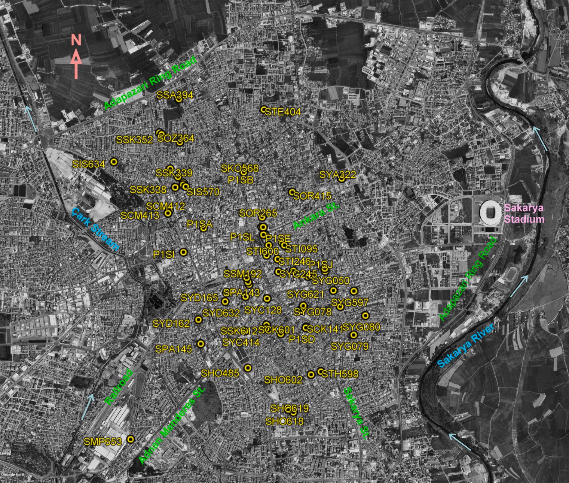
Fig. 2. Adapazari city centre and research points of the study.
ensemble learning (Alobaidi et al., 2019).
This study aims to understand the gray region between the different transition zones proposed liquefiable-non-liquefiable zone. ML models can be used to discover linear or nonlinear relationships. In this study, the advantages and effectiveness of ML models, including decision trees (DT), logistic regression (LOGREG), support vector machines (SVM), knearest neighbors (KNN), stochastic gradient descent (SGD), random forest (RF), and artificial neural network (ANN) for the prediction of soil liquefaction potential were investigated. Algorithms were coded in Python and applied to the dataset taken from the Adapazari/Turkey region after the 1999 Kocaeli earthquake. The main contribution of our work includes (i) Finding the best predictive model for soil liquefaction. (ii) An original data set (never used for machine learning) in Adapazari data
was modeled by ML models. (iii) Different ML models were tried for different parameters, and the best model was the decision tree algorithm. (iv) The model can be used in Adapazari soil samples. This paper is organized as follows: Section 2 presents the methodology and the proposed approaches, including data collection and characteristics. Also, it explains the details of the different machine learning methods. Section 3 presents the experimental results and performance comparison of the ML models. Finally, Section 4 presents the conclusions and possible future works.
2. Materials and methods
2.1. Study area and dataset
The field data results of many drillings and seismic cone penetration tests (SCPT) were collected in the dataset covering the entire city of Adapazarı, Turkey. In addition, classification and strength properties tests were carried out on the samples from the drillings and transferred to the database (Onalp et al., 2001; Bol et al., 2008, 2010). Bray et al. (2004) presented critical layers in Adapazarı where soil damage due to liquefaction was observed after the 1999 Kocaeli earthquake. These layers’ soil properties were taken from the report published on Pacific Earthquake Engineering Research Center (PEER) website and added to the database (Bray et al., 2001).
Soils can be formed in many different environments, including the main titles of residual and transported soils. Soil types that cause problems in geotechnical are generally soils formed by transport with thick layers. This type of soils can also be formed in very different facies and sub-facies environments. For example, moraines carried by glaciers, dunes formed by winds, talus formed by gravity and finally alluviums carried by water. Alluviums carried by water are considered to be of fluvial origin. In particular, the meandering river-based fluvial environments from which the soils used within the scope of this study originate carry very different sub-facies. For example, abandoned riverbed, set top deposits, cravasse splay deposits, oxbow lake deposits and flood plain deposits. The soils used in this study are also fluvialorigin flood plain sediments. The Adapazarı soils, from which the samples used in this study were taken, are flood plain sediments of fluvial
Fig. 3. A sample representation of the decision tree.
Fig. 4. Network Architecture of an MLP.
M. Ozsagir
5. Boxplots indicating the distribution of the features.
origin.
A large part of Adapazarı and its surroundings are formed by quaternary alluvial deposits containing gravelly and silty sands brought by
Fig.
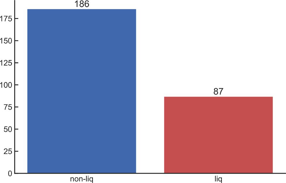
Fig. 6. Target value frequencies.
Fig. 7. 5-fold cross-validation method.
Fig. 8. Confusion matrix of the soil liquefaction potentials.
Table 4
Correlation matrix of the soil features.
Table 5
Selected hyperparameters of each algorithm.
DT max_depth: [3,4,5, ,20], min_samples_leaf: [3,4,5, ,20], criterion: [gini, entropy], splitter: [best, random], max_features: [auto, sqrt, log2]
LOGREG penalty: [l1, l2, none],C: np.linspace(-100, 100, 50)
, fit_intercept: [True, False], solver: [newton-cg, lbfgs, liblinear]
SVM kernel: [rbf, linear],C: np.linspace(-100, 100, 50) ,gamma: np.linspace (0, 100, 20)
KNN n_neighbors: [1,5,10, ,100], weights: [uniform, distance], leaf_size: [20, 25, , 100], p: [1, 2], algorithm: [auto, ball_tree, kd_tree, brute]
SGD loss: [hinge, log, modified_huber, squared_hinge, perceptron], penalty: [l1, l2, elasticnet],alpha: np.linspace(0.001, 100, 50)
, learning_rate: [constant, optimal, invscaling, adaptive], eta0: [1, 10, 100]
RF criterion: [gini, entropy], max_depth: [2,3,4, ,10], min_samples_split: [2,3,4, ,10], min_samples_leaf: [2,3,4, ,10], n_estimators: [2,3,4, ,10], max_features: [auto, sqrt, log2]
ANN hidden_layer_sizes: [(2,), (3,), (4,), (2, 2), (2, 3), (2, 4), (3,3),(3,4),(4,3),(4,4),(5,5),(6,6)], activation: [tanh, relu, logistic], solver: [sgd, adam], alpha: [0.0001, 0.001, 0.01, 0.1, 0.05], learning_rate: [constant, adaptive]
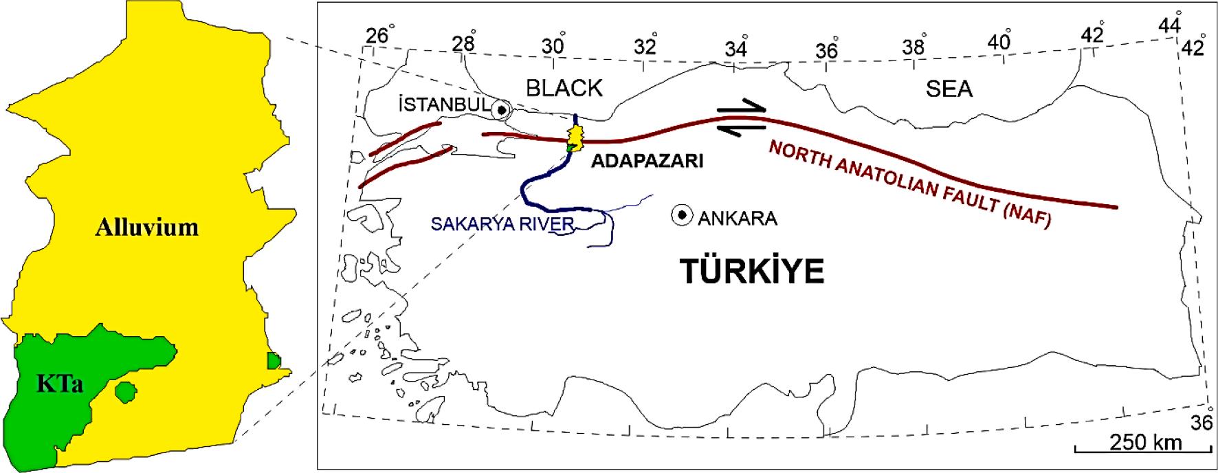
the Sakarya river. Different facies are observed to varying depths in different parts of the Adapazarı plain. A small section in the city’s southwest was founded on the cretaceous Akveren formation. The formation consists of claystone, sandstone, limestone, and marl layers. The densely populated areas are on the alluvial layers (Fig. 1). Adapazari city centre and research points of the study are shown in Fig. 2
In the initial dataset, presented in Table 2, includes soil samples taken from different points of the Adapazari region and 8 soil features. A column on whether the soil properties used caused soil liquefaction is also included in the data set with the binary values [0,1]. The value of “0” denotes non-liquefied, and ”1” denotes liquefied soils, which is known as the “target” variable in data science applications. The binary criterion of liquefaction/no-liquefaction was judged primarily based on surface manifestation of liquefaction, such as sand boils, ground settlement, and lateral spreading (or lack thereof), and in some cases (such as those reported by Bray et al. 2004; Bol et al. 2010), critical layers were identified by field observations supplemented with detailed dynamic finite element analyses or confirmed by multiple existing liquefaction
evaluation methods.
In the data preprocessing stage, the data missing any feature was detected and removed from the data set. At the same time, inconsistent data in the data set (- values, non-numerical, different typed data with the same meaning) was cleaned (cleansing). After the pre-processing stages, there is very little data left in the dataset that is inconsistent or noisy. Having missing values in a data set reduces the model performance (Kang, 2013). The statistical summary of the feature sets includes the mean, standard deviation (std), minimum (min), and maximum (max), which are presented in Table 3
2.2. Machine learning methods
Machine learning (ML) models, a subset of artificial intelligence, can be divided into three subgroups. These are supervised learning, unsupervised learning, and reinforced learning. Supervised learning is used when the target variables in the data set are known. In unsupervised learning, the values of the target variables are initially unknown (El Naqa & Murphy, 2015). The target variable discussed in this study, i.e., the potential for soil liquefaction will be given to the model. Therefore, supervised learning algorithms will need to be used. Supervised learning algorithms can be collected under regression and classification studies. The target variable in this study is binary, so the study will be treated as a classification study. In most studies, it can be determined by trialing different algorithms that will work better. The quality and quantity of data can be determined by looking at the relationship of characteristics in the data with each other to select appropriate machine learning algorithms (Zhang, 2020). After the relationships in the data are revealed, the data set is trained with parametric methods such as logistic regression, artificial neural networks, naive Bayes, or non-parametric methods such as k-nearest neighbors algorithm, decision trees, and support vector machines (Bonaccorso, 2017). If linear models can be used among the features in the data set, the model will work better with linear machine learning algorithms. The approaches to this study include both parametric and non-parametric methods, which are outlined below.
2.2.1. Decision trees
Decision tree algorithm (DT) is used for classification tasks in machine learning, and it can work with both categorical and continuous data. Thus, it has a more widespread use (Charbuty & Abdulazeez, 2021). DTs enable modeling in a tree structure that extends from the root to the leaves. The creation of the tree begins from the root. When determining the feature on the root node, the Gini index or entropy values are examined. The impurity status of the feature denotes a degree of inhomogeneity values. If the probability of a condition is pi , the entropy value (E) is calculated as follows (Breiman et al., 1984; Kingsford & Salzberg, 2008; Quinlan, 2014; Rokach & Maimon, 2005):
The formula for the Gini index (G) is estimated as:
These measures determine the impurity value of a feature. The feature selection process is completed by choosing the highest
Table 6 Best hyperparameter combinations for DT algorithm. criterion max_depth max_features min_samples_leaf
Table 7 Best
Table 8
Best hyperparameter combinations for SVM algorithm.
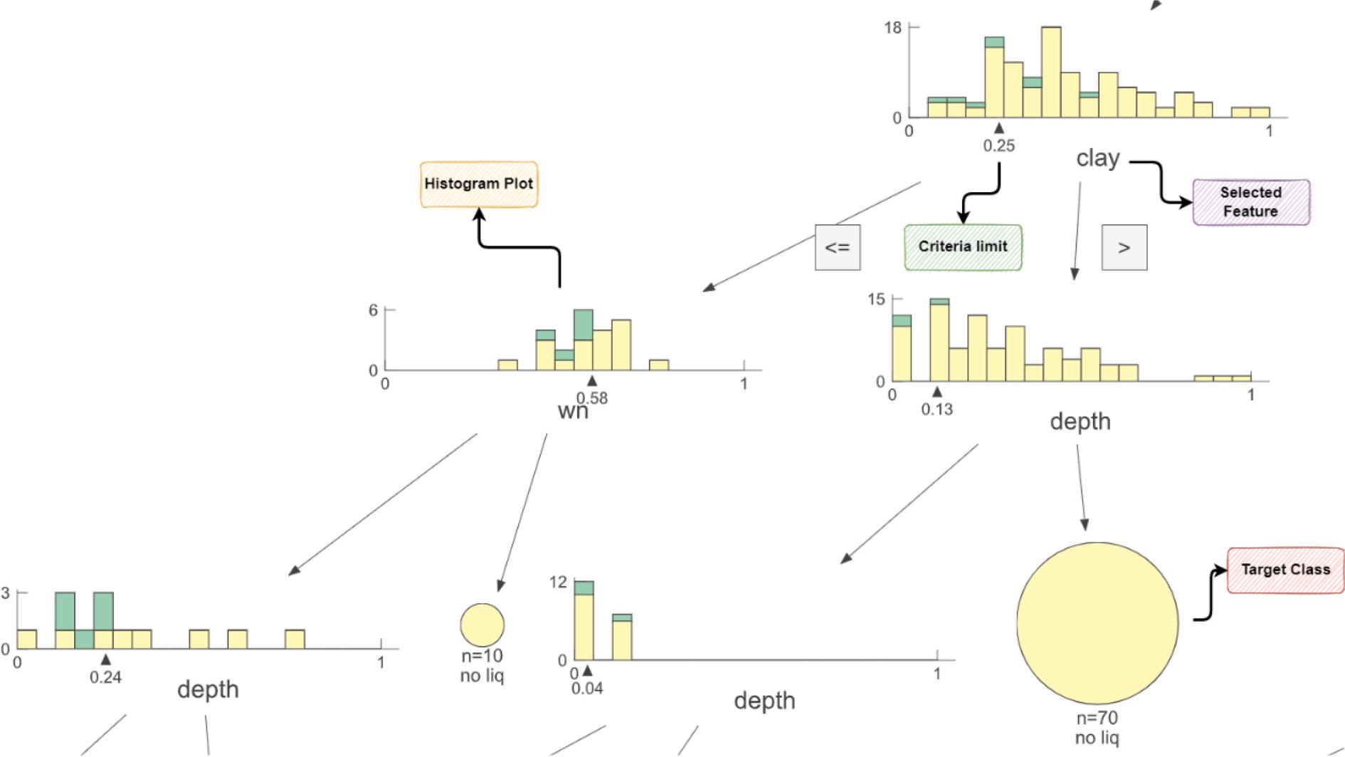
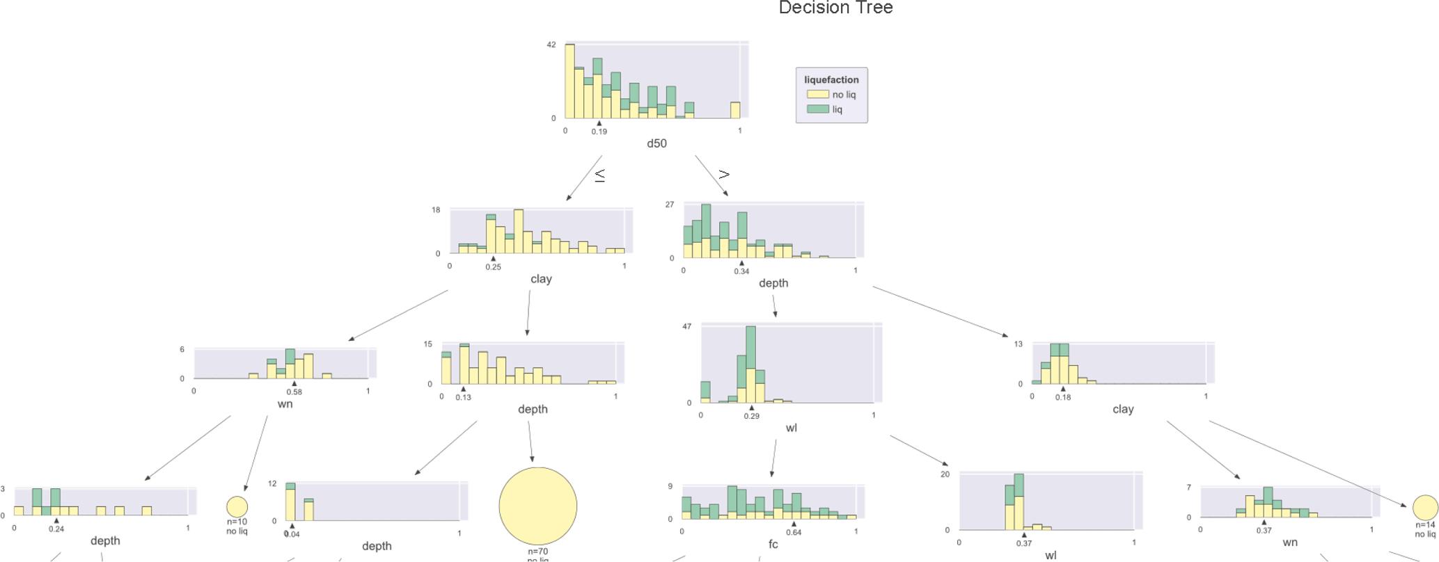
values because the feature with a high impurity value provides the most information gain. After deciding which feature to branch out in the decision tree, the criteria are determined. Criteria are branched out to see which number is more significant than smaller. If there is a 100 % class under the branch, the representation in that branch is completed. Fig. 2 is an example decision tree generated from the data in this study. Accordingly, clay has been selected as first branching feature. If clay is lower than 0.25, it should go to the left side(the wn side). Otherwise, in the right side, if depth is lower than 0.13, it should go to the left side. Otherwise, as a result of the branching to the right, the target class is determined as non-liquefied based on 70 samples.
2.2.2. Random forest
Learning is carried out by using a single tree in DT. Ensemble methods work with more than one tree. DTs may involve overfitting. The random forest algorithm performs training by working with some decision trees to prevent overfitting (Breiman, 2001). The random forest algorithm chooses the best by rating decision trees. The random forest algorithm is an algorithm that can be used instead of decision trees to avoid overfitting in high-size data sets. Other models developed with decision trees are boosting algorithms. In this study, ensemble decision trees were applied with random forest algorithms.
2.2.3. Support vector machines
Support vector machines (SVMs) are an algorithm classified by drawing boundary lines between classes (Joachims, 1998) used for both regression and classification problems (Mavroforakis & Theodoridis, 2006). SVM ensures the maximum distance between classes where boundary lines are drawn. Boundary lines of support vector machines are sometimes linear and sometimes work with high-sized kernels to predict more features.
2.2.4. K-nearest neighbors
K-Nearest Neighbors algorithm (K-NN) is another non-parametric classification algorithm. It can be used in both classification and regression (Altman, 1992). Because the K-NN algorithm is not parametric, it provides an excellent opportunity for data that does not fit a model. The most crucial parameter in the K-NN algorithm is the number of k, which specifies how many neighbors a point belongs to a class. In this study, the k coefficient in the KNN algorithm was tried with different parameters.
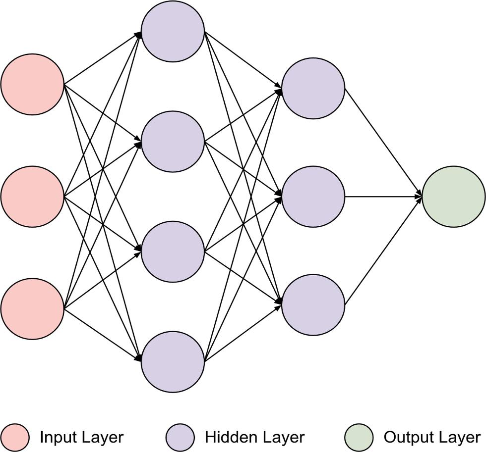
2.2.5. Artificial neural network (multilayer perceptron)
Artificial neural networks or multilayer perceptron (MLPs) consist of 3 layers: input, hidden, and output layers. MLPs may not have hidden layers. This case means that a simple artificial neural network (ANN) has been used. Besides, hidden layers can be used to detect more complex relationships. The number of units in the layers is one of the most critical parameters of these algorithms. The layers are entirely connected. Fig. 3 shows a representative artificial neural network.
2.2.6. Logistic regression
Linear regression models are used if the output variables are continuous. Logistic regression models have been developed to use regression models in classification problems. Intercept and slope values are estimated as linear regression in logistic regression (Hosmer et al.,
2013). A function is needed for the predicted value to be intermittent, a logistical function. Thanks to the logistics function, output values in linear regression are discontinuous. The resulting categorical variables indicate a class. The formula of the logistics function is given in Eq. (3).
L: max value of the curve k: logistic growth rate of the curve x0 : sigmoid’s midpoint x value
2.2.7. Stochastic gradient descent (SGD)
Stochastic gradient descent (SGD) is an iterative procedure applied in many machine learning studies. The algorithm SGD mimics Polyak’s heavy-ball method for the optimization problems (Polyak, 1964). SGD is a good and popular algorithm that has been implemented in well-known machine learning packages Pytorch (Ketkar & Moolayil, 2021) and Tensorflow (Dillon et al., 2017).
2.3. Data pre-processing
It is necessary to determine the practical factors in soil liquefaction to make the data set appropriate for machine learning applications. For this purpose, the factors determined by expert opinion are included in the data set. One essential pre-processing phase that improves the performance of machine learning algorithms is the scaling or normalization process. In this study, each feature is scaled with min–max scaling. Using Eqs. 4 and 5, the min–max scaling method scales the features to the range [0,1].
Xstd = X Xmin(axis 0) Xmax(axis 0) Xmin
here X is the original value, Xmin and Xmax the minimum and maximum value of the feature, respectively. Xscaled is the scaled value.
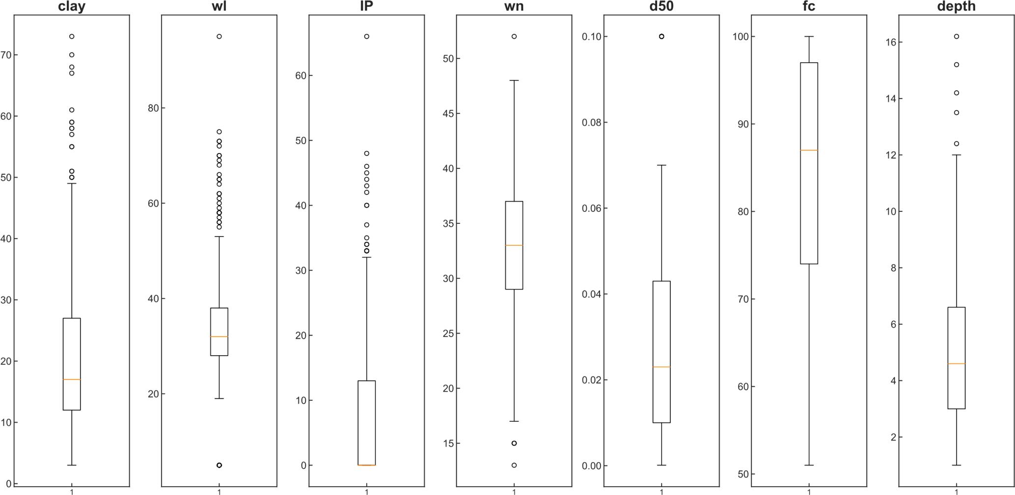
Boxplot graphs are drawn to detect outlier data (Fig. 4). Since the outlier data is not at the extremes, it was decided not to remove it from the model with expert opinion.
There are 186 data points for non-liquefied and 87 data points for liquefied soils in the data set, shown in Fig. 5. If dataset of machine learning applications is imbalanced (the number of observations in one target class is significantly lower than the number of observations in another class), this should be considered in training and test sets. F1score is the most approprite metric for calculating performance of the model (Eq. 9). If there are excessive classes in the training set, poor performance can be observed in the test set. Distributed data sets can be determined close to each other in training and test sets to eliminate this situation. In this study, since the entire data set is used in both training and verification using cross-validation, there is no need for a distributed data set preference close to each other.
The best model can be developed with cross-validation without relying on the training and test set in the data set. If only one training and test set is used, a good performance obtained by adhering to the
M. Ozsagir
Table 9 Best hyperparameter combinations for KNN algorithm. algorithm leaf_size n_neighbors p
Table 10 Best
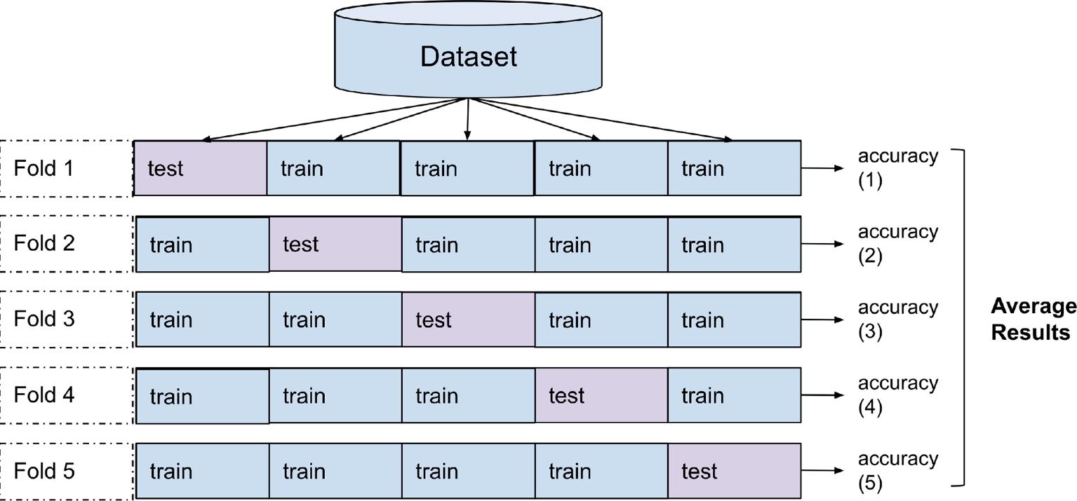
training set may not be generalized to the entire test set or data set. If the model produces results that are very close to the data in the training set but produce far-from-the-right results in the test set, the model may have ’overfitting’ memorization. If the model has low performance in the training set and high performance in the test set, which means the model is simple, called ‘underfitting’ The generalization of machine learning models is possible with hyperparameter optimization and crossvalidation methods. In cross-validation, the data set is divided into k subsets, then the k 1 set is used for training, and the other set is used for testing. In this study, the cross-validation data set was divided into five parts. In other words, 20 % validation and 80 % of the data set are used for training with each validation. Fig. 6 illustrates how to separate the data set into a training and test set in the cross-validation phase.
2.3.1. Performance metrics
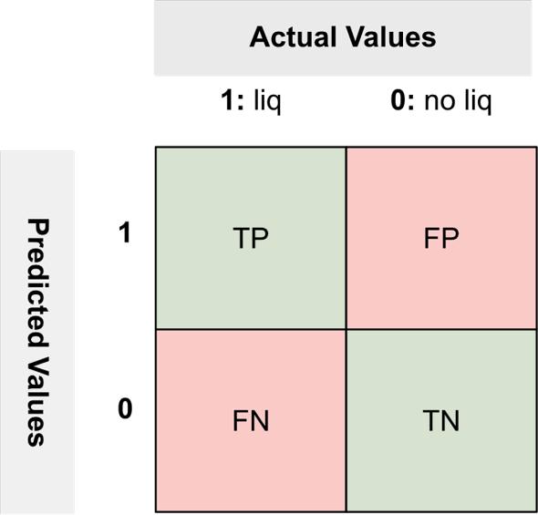
The model with the best average performance value in crossvalidation was used for modeling the data set. In the validation of the model, the data set split %80, %20 for the training and testing process, respectively. Moreover, the training accuracy, test accuracy, and accuracy of the entire data set were saved. Performance metrics were used to evaluate the performance of the model. Since the problem addressed is a binary classification problem, the confusion matrix consisting of a 4-cell window can be used for performance comparisons. Fig. 7 shows the confusion matrix for this study.
TP (True Positive): Correct predictions of liquefied soil.
TN (True Negative): Correct predictions of non-liquefied soil.
FP (False Positive): Incorrect predictions of liquefied soil.
FN (False Negative): Incorrect predictions of non-liquefied soil.
Accuracy is the most common performance metric used for binary classification problems. Another performance metric is the true positive rate (TPR) or recall, true positive predictions. Accuracy and the TPR are calculated using Eqs. 6–7:
Accuracy = TP + TN TP + TN + FP + FN (6)
Recall = TP TP + FN (7)
True Negative Rate (TNR) or Precision is the proportion of true negative predictions, which can be calculated by Eq. 8:
Precision = TN TN + FP (8)
F1-score or F-score or F-measure is the precision and recall weighted average. F1-score can be calculated by Eq. 9:
F1 = 2 × precision × recall precision + recall (9)
Area Under Curve (AUC), the Receiver Operating Characteristic (ROC) represents true positive and false-positive rates for different threshold values.
2.3.2. Feature selection
In the data preparation, incorrect data detection and cleaning, outlier data analysis, and incomplete data transactions were carried out. The data deemed contrary was removed from the data set by taking expert opinion to clean up the outlier data. In addition, the missing data has been removed from the data set because it is predicted that model performance will decrease due to filling in the missing data with one of the missing data filling methods.
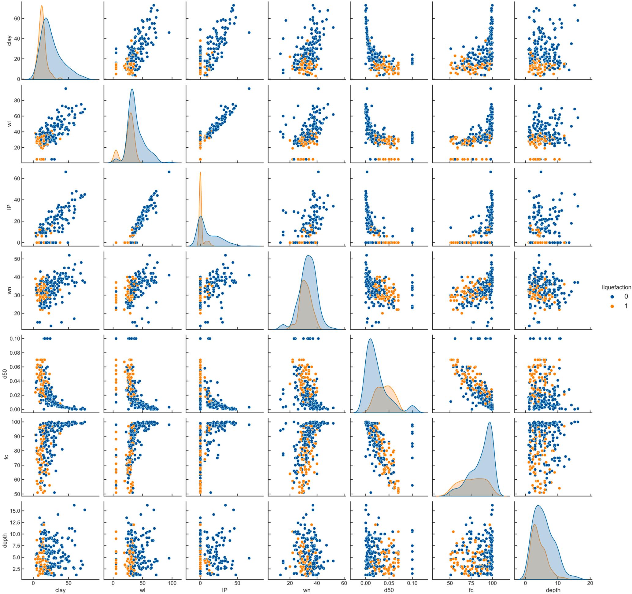
Scatter plots are given in Fig. 8 to show the distributions between properties and the target variable. As shown in Fig. 8, some features do not exhibit parametric distribution. When looking at the different feature values for liquefied and non-liquefied soils together, it was observed that it is impossible to make a linear distinction. Such situations will affect the performance of machine learning algorithms. It has Table 11 Best hyperparameter combinations for ANN algorithm.
Performance comparisons of the models. Models
been observed that the values of 0, especially in the IP feature, are in high numbers. In the laboratory, the plastic limit is difficult to measure on silty soils and is very dependent on the operator. In addition, the repeatability of the plastic limit test is one of the most difficult among geotechnical laboratory tests. Therefore, the IP feature is not considered
in many liquefaction criteria.
The correlation matrix was used for interactions between features (Table 4). If the correlation between the features is high, one of the features must be removed from the data set. In this study, it was aimed to work with as many features as possible. Therefore, feature with the Table 12
Fig. 9. Relation between features.
highest correlation(IP feature with a correlation of 0.86) is removed from dataset. So, the threshold value for this study was set as 0.85.
3. Results and discussion
The Scikit-Learn library was used in the Python programming language for machine learning models and codes developed for performance calculations in this study (Pedregosa et al., 2011). The experiments were done on a laptop with Intel(R) Core(TM) i7-5600U CPU @ 2.60 GHz and 12 GB RAM running 64-bit Windows. The data set discussed in the study is trained with 5-folds cross-validation. The average of the cross-validation results was taken and sorted according to different parameters using the Grid Search technique as an optimization method. Table 5 provides value ranges for the parameters used and the total number of experiments of each algorithm.
Models have been developed with the best parameters obtained due to cross-validation. Five of the best combinations obtained by Decision Tree (DT), Logistic Regression (LOGREG), Support Vector Machines (SVM), k-Nearest Neighbor (KNN), Stochastic Gradient Descent (SGD), Random Forest (RF), and Artificial Neural Network (ANN) crossvalidation are given as in Tables 6-11. The best parameter combination obtained with the parameters specified in the table will then be tried on the entire data set and added to the study’s outputs. Some hyperparameters combinations produced the same results. One of these combinations is presented in summary. The information presented in the tables shows an example of the best results. Performance evaluations
were made according to the average test accuracy score. CPU times of the algorithms were given as 64.5 s. 44.2 s 58.4 s 122.9 s 135.2 s 320 s respectively.
Models have been developed with the best parameters obtained due to cross-validation. The results obtained when the model has tried again in the randomly selected 20 % test set with the algorithm that gives the best result due to cross-validation are summarized in Table 12 The best overall accuracy for all dataset is 90 % was reached in the DT classifier. After the DT classifier, the RF classifier, a decision tree-based algorithm, comes in second place with an 86 % accuracy rate. According to table, DT obtained best accuracy rate in also precision (91 %), recall (96 %), and f1-score(93 %, 83 %). In addition, the results in which the RF algorithm can also be highlighted. RF obtained the best results on precision and recall rate.
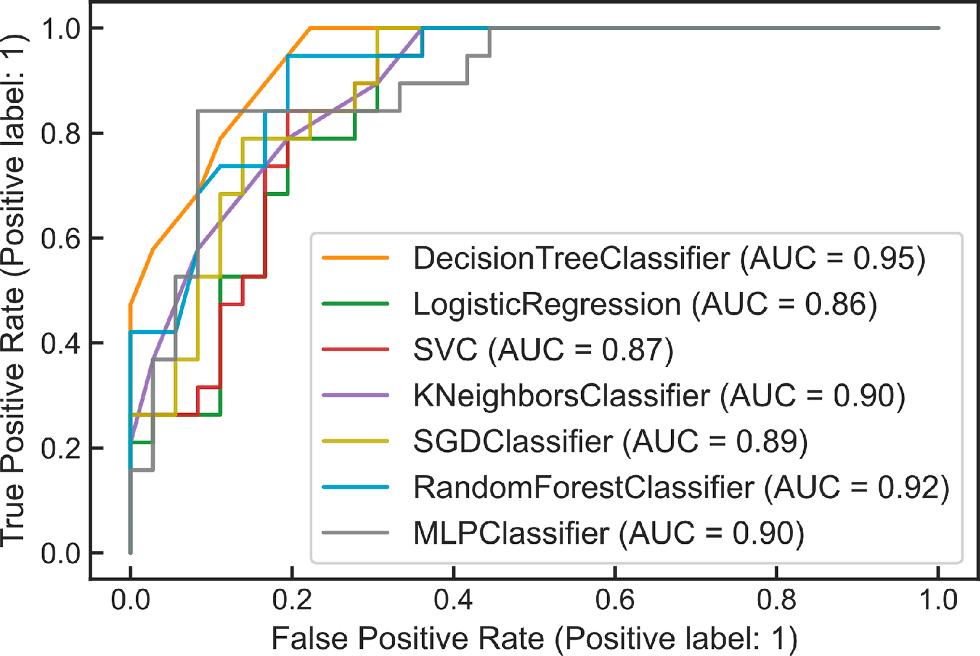
Another performance metric that is noted in this study is the ROC (Receiver Operating Characteristic) in which true positive rate is usually plotted on the Y axis, whereas false positive rate is plotted on the X axis. This suggests that the “ideal” point is in the upper left corner of the figure, with a false positive rate of zero and a true positive rate of one (scikit-learn, 2022). The true positive rate represents the percentage of liquefied soils that the model predicted as liquefied. Vice versa, false positive rate is the percentage of non-liquefied soils, but the model predicted them as liquefied soil. This metric summarizes the goodness of fit of a classifier. ROC curves for both training and test sets are given in Fig. 9. The best feasible prediction approach would result in a point in the upper left corner of the ROC space. A random guess would result in a
Fig. 10. ROC Curve for both test and train sets of the models.
Fig. 11. Best decision tree model visualization.
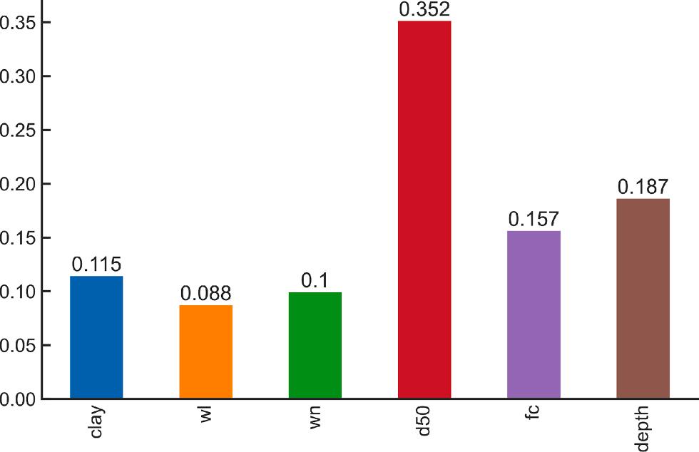
Fig. 12. Feature importance generated from DT model.
M. Ozsagir
point running diagonally from the bottom left to the top right corners. Looking at the ROC curves, it can be seen that the DT classifier again gives the best results with 97 % in the training set and 95 % in the test set best on various parameters. The RF classifier comes in second place.
According to the results given, it is concluded that the DT classifier can be used in the estimation of the potential for soil liquefaction. In the classification made with the decision tree, 178 non-liquefaction soil cases were correctly estimated. Conversely, 8 cases were incorrectly estimated. Sixty-seven samples from non-liquefaction soils were accurately estimated. By contrast, 20 cases were incorrectly estimated. The DT classifier is an algorithm that is easy to read and interpret. One of the outputs of the algorithm is the rules of decision. Decision rules can be created to predict new data. A few of the decisions considered important are shown in Fig. 10.
Moreover, D50 feature is found as the first splitting attribute, as shown in Fig. 11 That’s why D50 indicates the most important feature in the dataset. As mentioned, D50 had the strongest effect on the liquefaction prediction in the case of DT model, while the depth feature had the second strongest effect. The relative importance of each feature for predicting soil liquefaction is given in Fig. 12
The limit values were calculated by inverse scaling so that the results could be evaluated with their actual values. The important decision rules are summarized as follows:
• if (d50 <= 0.01948) and (clay > 20.5) and (depth > 2.9) then class: no liq (proba: 100.0 %) | based on 70 samples
• if (d50 > 0.01948) and (depth <= 6.1528) and (wl <= 31.45) and (fc <= 82.507) and (depth <= 4.4504) and (d50 > 0.03296) and (clay <= 14.48) and (d50 <= 0.0595) then class: liq (proba: 100.0 %) | based on 17 samples
• if (d50 > 0.01948) and (depth > 6.1528) and (clay > 15.53) then class: no liq (proba: 100.0 %) | based on 14 samples
• if (d50 <= 0.01948) and (clay <= 20.5) and (wn > 0.577) then class: no liq (proba: 100.0 %) | based on 10 samples
• if (d50 <= 0.01948) and (clay > 20.5) and (depth <= 1.5472) then class: no liq (proba: 100.0 %) | based on 9 samples
• if (d50 > 0.01948) and (depth <= 6.1528) and (wl > 31.45) and (wl <= 38.48) and (wn <= 38.506) and (d50 <= 0.055) and (fc <= 93.483) and (wl <= 35.95) and (fc > 88.485) then class: no liq (proba: 100.0 %) | based on 6 samples
• if (d50 <= 0.01948) and (clay > 20.5) and (depth <= 2.9) and (depth > 1.5472) and (d50 <= 0.0059) then class: no liq (proba: 100.0 %) | based on 6 samples
4. Conclusions
This study presents a model for soil liquefaction potential using seven well-known machine learning approaches: DT, LOGREG, SVM, KNN, RF, ANN, and SGD. The Adapazarı data set is trained after being evaluated with expert opinion and passed through the pre-processing stages. In the training process, the results of the algorithms with different parameters were recorded. Thus, algorithms with the best parameters are provided with better results. When the algorithms used were sorted according to the quality of training of the entire data set, it was observed that the decision trees obtained the highest results with an accuracy 90 % success rate. The results obtained by the RF classifier were the second-best algorithm. The specified DT model resulted in 91 % accuracy in the randomly selected training set and 84 % accuracy in the test set. F1 score of the DT model reached 96 %. The rules, which previously stated whether there was liquefaction with expert opinion, were developed by machine learning methods. DT model in this study presents a good alternative for the prediction of liquefaction and gives more accurate results than the previous works. However, many methods in the literature offer a test site where the decision cannot be made as soon as it liquefies. Decision rules produced with decision trees are proposed in the results and discussion section. To sum up, soil
liquefaction decisions can be made using these rules. In addition, the importance of the features in the data set discussed was determined by decision trees. Accordingly, the feature ranking was discovered as D50, depth, FC, clay, wn, wL
The Adapazarı soils, from which the samples used in this study were taken, are flood plain sediments of fluvial origin. Since the precipitation pattern is the same in such environments all over the world, the results obtained within the scope of the study can also be used in environments with similar formation conditions. When it is desired to be used on soils with different formation conditions, the results should be confirmed by different methods.
The studies that can be done after this study can be summarized as follows:
- The model will decide whether the new data has soil liquefaction potential with a web interface.
- The model can be compared with deep learning methods. Due to the small number of data, this study has not utilized deep learning methods.
- Fuzzy, coarse, and gray clusters can be used for soil liquefaction modeling.
CRediT authorship contribution statement
Mustafa Ozsa ˘ gır: Conceptualization, Methodology, Writing – original draft, Writing – review & editing. Caner Erden: Software, Methodology, Visualization, Data curation, Writing – original draft. Ertan Bol: Methodology, Data curation, Writing – review & editing, Investigation, Supervision. Sedat Sert: Writing – review & editing, Supervision. As ¸ kın Ozocak: Writing – review & editing, Supervision.
Declaration of Competing Interest
The authors declare that they have no known competing financial interests or personal relationships that could have appeared to influence the work reported in this paper.
Data availability
The authors do not have permission to share data.
References
Ahmad, M., Tang, X.-W., Qiu, J.-N., Ahmad, F., Gu, W.-J., 2021. Application of machine learning algorithms for the evaluation of seismic soil liquefaction potential. Front. Struct. Civ. Eng. 15 (2), 490–505. https://doi.org/10.1007/s11709-020-0669-5
Alobaidi, M.H., Meguid, M.A., Chebana, F., 2019. Predicting seismic-induced liquefaction through ensemble learning frameworks. Scientific Reports 9 (1), 11786. https://doi.org/10.1038/s41598-019-48044-0
Altman, N.S., 1992. An Introduction to Kernel and Nearest-Neighbor Nonparametric Regression. Am. Statist. 46 (3), 175–185. https://doi.org/10.1080/ 00031305.1992.10475879
Andrews, D.C., Martin, G.R., 2000. Criteria for liquefaction of silty soils. Proc., 12th World Conf. on Earthquake Engineering, 1–8.
Andrus, R.D., Stokoe, K.H., 2000. Liquefaction resistance of soils from shear-wave velocity. J. Geotech. Geoenviron. Eng. 126 (11), 1015–1025
Bol, E., Onalp, A., Ozocak, A., 2008. The liquefiability of silts and the vulnerability map of Adapazari. Proceedings of The 14th World Conference on Earthquake Engineering, October 12–17, 2008, Beijing, China
Bol, E., Onalp, A., Arel, E., Sert, S., Ozocak, A., 2010. Liquefaction of silts: The Adapazari criteria. Bull. Earthquake Eng. 8 (4), 859–873
Bonaccorso, G., 2017. Machine learning algorithms. Packt Publishing Ltd.
Bray, J. D., Sancio, R. B., Youd, L. F., Christensen, C., Cetin, K. O., Onalp, A., Durgunoglu, T., Stewart, J. P. C., Seed, R. B., 2001. Documenting Incidents of Ground Failure Resulting from the August 17, 1999 Kocaeli, Turkey Earthquake. Pacific Earthquake Engineering Research Center Website: Http://Peer. Berkeley. Edu/Turkey/ Adapazari.
Bray, J.D., Sancio, R.B., 2006. Assessment of the liquefaction susceptibility of finegrained soils. J. Geotech. Geoenviron. Eng. 132 (9), 1165–1177
Bray, J.D., Sancio, R.B., Durgunoglu, T., Onalp, A., Youd, T.L., Stewart, J.P., Seed, R.B., Cetin, O.K., Bol, E., Baturay, M.B., Christensen, C., Karadayilar, T., 2004. Subsurface characterization at ground failure sites in Adapazari, Turkey. J. Geotech. Geoenviron. Eng. 130 (7), 673–685
M. Ozsagir
Breiman, L., 2001. Random Forests. Machine Learning 45 (1), 5–32. https://doi.org/ 10.1023/A:1010933404324
Breiman, L., Friedman, J., Stone, C.J., Olshen, R.A., 1984. Classification and regression trees. CRC Press
Charbuty, B., Abdulazeez, A., 2021. Classification based on decision tree algorithm for machine learning. J. Appl. Sci. Technol. Trends 2 (01), 20–28
Dillon, J.V., Langmore, I., Tran, D., Brevdo, E., Vasudevan, S., Moore, D., Patton, B., Alemi, A., Hoffman, M., Saurous, R.A., 2017. Tensorflow distributions. ArXiv Preprint ArXiv:1711.10604
El Naqa, I., Murphy, M.J., 2015. What is machine learning?. In: Machine Learning in Radiation Oncology. Springer, pp. 3–11 Feng, Y., Cui, N., Hao, W., Gao, L., Gong, D., 2019. Estimation of soil temperature from meteorological data using different machine learning models. Geoderma 338, 67–77. https://doi.org/10.1016/j.geoderma.2018.11.044.
Finn, W.D., Ledbetter, R.H., Wu, G., 1994. Liquefaction in silty soils: Design and analysis. Ground Failures Under Seismic Conditions 51–76 García, S., Ovando-Shelley, E., Guti´ errez, J., García, J., 2012. Liquefaction Assessment through Machine Learning Approach. 15th World Conf. Earthq. Eng Goh, A.T.C., Goh, S.H., 2007. Support vector machines: Their use in geotechnical engineering as illustrated using seismic liquefaction data. Comput. Geotech. 34 (5), 410–421. https://doi.org/10.1016/j.compgeo.2007.06.001
Hosmer, D.W., Lemeshow, S., Sturdivant, R.X., 2013. Applied logistic regression. John Wiley & Sons
Hu, J., 2021. A new approach for constructing two Bayesian network models for predicting the liquefaction of gravelly soil. Comput. Geotech. 137, 104304 https:// doi.org/10.1016/j.compgeo.2021.104304
Jennings, P.C., 1980. Earthquake Engineering and Hazards Reduction in China: A Trip Report of the American Earthquake Engineering and Hazards Reduction Delegation National Academy of Sciences, Washington, DC
Joachims, T., 1998. Making large-scale SVM learning practical. Technical Report Kang, H., 2013. The prevention and handling of the missing data. Korean J. Anesthesiol. 64 (5), 402 Ketkar, N., Moolayil, J., 2021. Introduction to pytorch. In: Deep learning with python Springer, pp. 27–91
Kingsford, C., Salzberg, S.L., 2008. What are decision trees? Nature Biotechnol. 26 (9), 1011–1013
Koester, J.P., 1994. The influence of fines type and content on cyclic strength. Ground Failures Under Seismic Conditions 17–33. Kramer, S.L., 1996. Geotechnical earthquake engineering. Prentice Hall Upper Saddle River, New Jersey
Kumar, D., Samui, P., Kim, D., Singh, A., 2021. A Novel Methodology to Classify Soil Liquefaction Using Deep Learning. Geotech. Geol. Eng. 39 (2), 1049–1058. https:// doi.org/10.1007/s10706-020-01544-7
Lee, K.L., Seed, H.B., 1967. Drained strength characteristics of sands. J. Soil Mech. Found. Division 93 (6), 117–141 Makasis, N., Narsilio, G.A., Bidarmaghz, A., 2018. A machine learning approach to energy pile design. Comput. Geotech. 97, 189–203 Mavroforakis, M.E., Theodoridis, S., 2006. A geometric approach to support vector machine (SVM) classification. IEEE Trans. Neural Networks 17 (3), 671–682. https://doi.org/10.1109/TNN.2006.873281
Onalp, A., Arel, E., Bol, E., 2001. A General assessment of the effects of 1999 Earthquake on the soil-structure interaction in Adapazari In: Jubilee Papers in Honor of Prof. Dr. Ergun Togrol, XVth ICSMFE, Istanbul, Turkey, pp 77–89. Park, S.-S., Ogunjinmi, P.D., Woo, S.-W., Lee, D.-E., 2020. A Simple and Sustainable Prediction Method of Liquefaction-Induced Settlement at Pohang Using an Artificial
Neural Network. Sustainability 12 (10), 4001. https://doi.org/10.3390/ su12104001
Pathak S. R., Purandare A. S. Liquefaction susceptibility criterion of fine grained soil. International Journal of Geotechnical Engineering 10, sy 5 (2016): 445-59.
Pedregosa, F., Varoquaux, G., Gramfort, A., Michel, V., Thirion, B., Grisel, O., Blondel, M., Prettenhofer, P., Weiss, R., Dubourg, V., Vanderplas, J., Passos, A., Cournapeau, D., Brucher, M., Perrot, M., Duchesnay, E., 2011. Scikit-learn: Machine Learning in Python. J. Machine Learning Res. 12, 2825–2830
Polito, C.P., 1999. The effects of non-plastic and plastic fines on the liquefaction of sandy soils. Virginia Polytechnic Institute and State University
Polito C. P., and James R. Martin II. Effects of Nonplastic Fines on the Liquefaction Resistance of Sands. Journal of Geotechnical and Geoenvironmental Engineering 127, no. 5 (2001): 408–15.
Polyak, B.T., 1964. Some methods of speeding up the convergence of iteration methods. Ussr Comput. Math. Math. Phys. 4 (5), 1–17.
Quinlan, J.R., 2014. C4. 5: Programs for machine learning. Elsevier. Rokach, L., Maimon, O., 2005. Decision trees. In: Maimon, O., Rokach, L. (Eds.), Data Mining and Knowledge Discovery Handbook. Springer-Verlag, New York, pp. 165–192
Samui, P., Sitharam, T.G., 2011. Machine learning modelling for predicting soil liquefaction susceptibility. Natural Hazards Earth Syst. Sci. 11 (1), 1–9. https://doi. org/10.5194/nhess-11-1-2011
Sancio, R.B., Bray, J.D., Stewart, J.P., Youd, T.L., Durgunoǧlu, H.T., Onalp, A., Seed, R. B., Christensen, C., Baturay, M.B., Karadayılar, T., 2002. Correlation between ground failure and soil conditions in Adapazari, Turkey. Soil Dynamics Earthquake Eng. 22 (9–12), 1093–1102
Scikit-Learn, 2022. Receiver Operating Characteristic (ROC) Scikit-Learn. https://scikit-le arn/stable/auto_examples/model_selection/plot_roc.html
Seed, R.B., Cetin, K.O., Moss, R.E., Kammerer, A.M., Wu, J., Pestana, J.M., Riemer, M.F., Sancio, R.B., Bray, J.D., Kayen, R.E., 2003. Recent advances in soil liquefaction engineering: A unified and consistent framework. Proceedings of the 26th Annual ASCE Los Angeles Geotechnical Spring Seminar: Long Beach, CA
Seed, H.B., 1982. Ground motions and soil liquefaction during earthquakes. Earthquake engineering research insititue
Seed, H.B., Idriss, I.M., 1967. Analysis of soil liquefaction: Niigata earthquake. J. Soil Mech. Found. Division 93 (3), 83–108
Seed, H.B., Idriss, I.M., 1971. Simplified procedure for evaluating soil liquefaction potential. J. Soil Mech. Found. Division 97 (9), 1249–1273.
Seed, H.B., Idriss, I.M., Arango, I., 1983. Evaluation of liquefaction potential using field performance data. J. Geotech. Eng. 109 (3), 458–482
Seed, H.B., Tokimatsu, K., Harder, L.F., Chung, R.M., 1985. Influence of SPT procedures in soil liquefaction resistance evaluations. J. Geotech. Eng. 111 (12), 1425–1445
Taghizadeh-Mehrjardi, R., Hamzehpour, N., Hassanzadeh, M., Heung, B., Ghebleh Goydaragh, M., Schmidt, K., Scholten, T., 2021. Enhancing the accuracy of machine learning models using the super learner technique in digital soil mapping. Geoderma 399, 115108. https://doi.org/10.1016/j.geoderma.2021.115108
Tung, A.T.Y., Wang, Y.Y., Wong, F.S., 1993. Assessment of liquefaction potential using neural networks. Soil Dyn. Earthquake Eng. 12 (6), 325–335
Wang, W., 1979. Some findings in soil liquefaction Earthquake Engineering Department, Water Conservancy and Hydroelectric Power.
Youd, T.L., Idriss, I.M., 2001. Liquefaction resistance of soils: Summary report from the 1996 NCEER and 1998 NCEER/NSF workshops on evaluation of liquefaction resistance of soils. J. Geotech. Geoenviron. Eng. 127 (4), 297–313
Zhang, X.-D., 2020. Machine Learning. In: Zhang, X.-D. (Ed.), A Matrix Algebra Approach to Artificial Intelligence. Springer Singapore, Singapore, pp. 223–440
Another random document with no related content on Scribd:
bridges, machine tool workers, tinsmiths, iron and steel workers, electricians, telephone mechanics, steamfitters, plumbers, airplane and parachute makers and mechanics, railroad and transportation workers, roofers, radio, refrigeration and air conditioning mechanics, fireproofing and insulation workers, shoemakers, tailors, dressmakers, milliners, hat makers, and hundreds of other workers that we can keep busy provided that we always try to construct, improve, and expand, to produce and build, and to better the conditions, convenience, and comfort of us all."
"Do I understand that you will obtain all this without paying for it and that all of you will live on the same standard, regardless of the better workmanship and ability of others of you?" The President questioned, "And how will you compensate those of you who excel in their endeavors, and others of you who may invent an important mechanical improvement, discover the cure for a disease, or contrive some chemical development which will save labor and materials. In other words, what incentive will any of you have to excel?"
"I was expecting that question. First, as I have mentioned before, every one of us will get our house, our food, and all of life's necessities absolutely free; second, we will copy the system of the Martians. We will have ten lower degrees and ten higher ones. The higher ones we will call rank degrees. There will be ten points between one degree and another and we will be gradually and honorably promoted or demoted by points the same as we were in the army. Those who have made a discovery, an invention or a needful improvement and those who have done meritorious service will receive for life a better, larger, and more comfortable home in the suburbs outside the city, with certain luxuries such as a better and larger plane and luxurious pleasure automobiles. They will have the services of attendants in their homes; first production and best quality of all our necessities, and many other compensations and honors that our authorities will decree. On the other hand, we will demote and punish any one who, through malicious intent, will not obey our laws and regulations or will not comport himself honorably according to our rules.
"We and many others of our returned soldiers and sailors who have just served and fought in the bloodiest of world battles, and we, with our buddies, who sacrificed themselves on the battlefields, were the instruments in this most atrocious war. The victims of inhuman hellish, cruel warfare, we experienced and endured the ordeals of the greatest sufferings that human flesh and fortitude can stand in battles.
"We fought on the blood-soaked decks and gun-turreted floors of battleships, in the fuselage, cockpit, bellies, and wings of flying fortresses, inside hot, cramped, fire-and-cannon belching tanks, in the putrified trenches and shell and fox holes of battle scarred beaches, on the sides of most inaccessible steep mountain precipices, and on deserts and in jungles where we lay day and night in putrid mud, water, and scum. We faced blinding, blazing sun, terrific heat, torrential rains, and body-freezing snow blizzards. We suffered from frost bites, lack of sleep, hunger, and thirst, surrounded by dirt and bitten by insects, vermin, and reptiles during the agonies of our painful wounds. We constantly heard the anguishing, pleading and moaning of men lying wounded on No Man's Land. Before our very eyes, our buddies and brothers and best friends were shot and torn asunder. Others had their eyes gouged out and hanging over their cheeks. Many of our paratroopers were used as clay pigeons and by mistake shot down by our own soldiers. At any moment we were expecting to meet their fate. Many of our buddies were destroyed like a puff of smoke, whose only remains and memories are the star medals worn by their mothers.
"We were like a pack of maddened wolves with the strength, daring, and fearlessness of lunatics. With diabolical fury, we darted and bounded wildly and fearlessly into No Man's Land in the face of the greatest danger.
"Timid ones became heroes without knowing it. The weakest ones killed with their bare hands. It was indescribable! All of us became filthy, cruel, inhuman beasts, with fierce irrational emotions and the sole urge to kill, kill, and kill our enemy. We fought to the death with
no quarter asked or given. Most of us were mumbling our prayers or the names of our beloved. It is really a miracle that those of us who came out alive from this vertex of blood and slaughter are again normal and human.
"Closing his eyes, kneeling, passionately weeping, and vehemently imploring, he exclaims—In my mind's eye I see passing in front of me, the lost souls, images of dead soldiers, some of the countless billions of them who died on the battlefields of our earth.
"Their spirits are joining and inspiring me in this solemn entreaty for you to help us, so that their sacrifices shall not have been in vain. Standing up, he continued:
"What of the great many of us who survived, but who are maimed, crippled, invalidated, disfigured and shell shocked for life? The terrible pictures of our battle sufferings recur to us very often in our dreams. Through our torments, tortures, and ordeals, we have learned in the hardest way the contributive whys and causes of wars and inhumanity.
"Labor and capital struggles, strikes, unemployment, racial hatred, and misery are becoming burdensome and unbearable to the majority of us in this world. In our military life, in the army, in our company, and on the battlefields, we lived unselfishly as brothers and buddies. We loved each other, judged each other on our merits, and forgave each other our frailties and weaknesses.
"Now that we have re-entered civilian life, it is irksome to us to adjust ourselves and face an existence of selfishness, where the main object in life is personal interest, regardless of those others. Nature has endowed us with intelligence; on account of it we are humane, helpful, unselfish, and self-sacrificing for the welfare of our kind. Our ancestors have planted on us a money system, a most heartless, dangerous, tempting, criminally corrupting, degrading, and depraving medium without which we cannot obtain our necessities.
"In the last war we who endured agonies were used as tools for gaining victory in war for a partof humanity. Now, we are anxious to be used as implements for gaining universal salvation for all humanity. By our test and peaceful experiment which we ask you to allow, we hope to exemplify the new order which will achieve universal and lasting peace by destroying the real causes and incentives for crime and for all cruel wars with its wanton disregard of human life, and thereby save humanity.
"On our planet, in three successive progressive changes, with each consecutive variation, we increased and intensified our armed war conflict cruelties against each other.
"First, the stone age, then the iron age and now we have with us, appalling atomic, gas and bacterial warfare. Help us to once and for all make an end to them. 'Tempora mutantur, et nos mutamur in illis'—The times are changed, and we are changed with them. You as the head of a leading world nation by such an act, example, and pattern to humanity, you will the sooner bring about the brotherhood of all men, and world security. A showdown is getting nearer, help us to forestall it.
"Please! Please! Mr. President, grant us these four islands for world experimental stations and laboratories, now so indispensable. Let them and us be the testing grounds and mediums in a new and better plan and ways of human conduct, relationship, intercourse, culture, and an economic system for the unlimited benefit of all mankind."
The President said, "I would suggest that you have our Congressmen here with the one that visited Mars who has observed their mode of life, present a Bill to Congress so that it be passed. I will sign it, and good luck to you!"
"We all hope that Congress will pass this Bill, and if our experiment of improved new economic ideas prove satisfactory, adjoining islands and peoples may join us, extending our influence. Then the United States will gain world leadership, and other nations will imitate us.
Therefore you and Congress will gain eternal honor, and fame in history and posterity, as the saviors of humanity, and the time may come, I hope, when there will be a gradual peaceable absorption of all earth's inhabitants to our way without undue pressure or strife that one world government will come into being, and a new life and the emancipation of all will bring happiness in 'OurComingWorld.'"
About two weeks after our return, a mysterious package attached to a small parachute of a strange design and fabric was seen floating down from the skies at La Guardia airfield. In it were found letters written on strange paper, enclosed in unstamped matching envelopes. One of them was addressed to me from Lieutenant Balmore; eleven other letters were addressed to his and his crew members' parents.
There was also a portfolio crammed with money, jewelry, and papers. Included were the last wills and testaments and transfer of properties of the crew, appointing me as executor and providing directions for turning over as soon as possible moneys and valuables and all their earthly possessions to their respective families. In his letter Lieutenant Balmore described his happy marriage with his beloved Xora, as well as the marriages of his crew members with beautiful Martian maidens of their choice, performed in one grand ceremony.
As another expression of his gratitude he writes: "Our opportune acquaintance, with our trips to Mars, was a very auspicious event, not only for us but with our efforts and your book a momentous opportunity to promote the deliverance of my former fellow Earthmen. My crew members join me in not only being very thankful, but also greatly obligated for the sincere faith you had in me, and it is due to your wholehearted support, that we are now the happiest men in the universe."
He enclosed a copy of announcements of large front page headlines which were in all Martian newspapers as follows:
"A RED LETTER DAY ON MARS"
"Today took place the unprecedented, extraordinary occurrence marking the beginning of a new and momentous era. Eleven Earth youths were married to eleven of our maidens. These couples were joined in a grand nuptial ceremony at one wedding attended by all the high dignitaries of our planet."
*** END OF THE PROJECT GUTENBERG EBOOK OUR COMING WORLD ***
Updated editions will replace the previous one—the old editions will be renamed.
Creating the works from print editions not protected by U.S. copyright law means that no one owns a United States copyright in these works, so the Foundation (and you!) can copy and distribute it in the United States without permission and without paying copyright royalties. Special rules, set forth in the General Terms of Use part of this license, apply to copying and distributing Project Gutenberg™ electronic works to protect the PROJECT GUTENBERG™ concept and trademark. Project Gutenberg is a registered trademark, and may not be used if you charge for an eBook, except by following the terms of the trademark license, including paying royalties for use of the Project Gutenberg trademark. If you do not charge anything for copies of this eBook, complying with the trademark license is very easy. You may use this eBook for nearly any purpose such as creation of derivative works, reports, performances and research. Project Gutenberg eBooks may be modified and printed and given away—you may do practically ANYTHING in the United States with eBooks not protected by U.S. copyright law. Redistribution is subject to the trademark license, especially commercial redistribution.
START: FULL LICENSE