Full Download Weather, macroweather, and the climate : our random yet predictable atmosphere lovejoy
Weather, macroweather, and the climate : our random yet predictable atmosphere Lovejoy
Visit to download the full and correct content document: https://ebookmass.com/product/weather-macroweather-and-the-climate-our-random-y et-predictable-atmosphere-lovejoy/
More products digital (pdf, epub, mobi) instant download maybe you interests ...
Thermal Physics of the Atmosphere 1 (Developments in Weather and Climate Science 1) 2nd Edition Maarten H.P. Ambaum
Oxford University Press is a department of the University of Oxford. It furthers the University’s objective of excellence in research, scholarship, and education by publishing worldwide. Oxford is a registered trade mark of Oxford University Press in the UK and certain other countries.
Published in the United States of America by Oxford University Press 198 Madison Avenue, New York, NY 10016, United States of America.
All rights reserved. No part of this publication may be reproduced, stored in a retrieval system, or transmitted, in any form or by any means, without the prior permission in writing of Oxford University Press, or as expressly permitted by law, by license, or under terms agreed with the appropriate reproduction rights organization. Inquiries concerning reproduction outside the scope of the above should be sent to the Rights Department, Oxford University Press, at the address above.
You must not circulate this work in any other form and you must impose this same condition on any acquirer.
CIP data is on file at the Library of Congress ISBN 978–0–19–086421–7
Printed by Sheridan Books, Inc., United States of America
List of boxes
Preface
Acknowledgments
1 Zooming through scales by the billion 1
1.1 What is weather? What is climate? 1
1.1.1 High level or low level? 1
1.1.2 Space and time 12
1.2 Zooming in time: The age of Earth to milliseconds 20
1.2.1 Paleoindicators 20
1.2.2 Instrumental temperatures 21
1.3 Zooming in space: From the size of the planet and from the top to the bottom 23
1.3.1 Horizontal 23
1.3.2 Vertical 24
1.4 The unfinished nonlinear revolution: Junk your old equations and look for guidance in clouds . . . 28
1.4.1 The development of numerical models 28
1.4.2 The nonlinear backlash 30
1.4.3 Complexity science 33
1.5 An overview of this book 34
2 New worlds versus scaling: From van Leeuwenhoek to Mandelbrot 40
2.1 Scalebound thinking and the missing quadrillion 40
2.1.1 New worlds and spectral bumps 40
2.1.2 New worlds and the meteorological zoo 55
2.2 Scaling: Big whirls have little whirls and little whirls have lesser whirls 56
2.2.1 The fractal revolution 56
2.2.2 Fractal sets and dimensions 59
2.2.3 Fractal lines and wiggliness 66
2.2.4 Richardson 74
2.3 Fluctuation analysis as a microscope 80
3 How big is a cloud? 95
3.1 Fractals: Where’s the physics? 95
3.1.1 Symmetries 95
3.1.2 Zooming and squashing 98
3.2 Zooming, squashing, and rotating, and the emergence of scale 106
3.2.1 The scaling of the laws 106
3.2.2 What is scale? 107
3.2.3 What about real clouds? 113
3.2.4 Simulating anisotropic scaling, fractals, and clouds 115
3.2.5 The 23/9 D model 117
3.2.6 The emergence of scale 120
3.3 Zooming with squashing and rotation, and the phenomenological fallacy 120
3.3.1 Generalized scale invariance 120
3.3.2 Anisotropic multifractals 124
3.3.3 Anisotropy that changes from place to place as well as scale to scale: Nonlinear GSI 131
3.3.4 The phenomenological fallacy 135
4 The weather: Nothing but turbulence . . . and don’t mind the gap 142
4.1 Turbulence and the mesoscale 142
4.2 A convenient gap and Richardson’s posthumous vindication 149
4.3 Science: A human enterprise 152
4.4 The rise of nonlinear geoscience 158
4.5 The triumph of scaling stratification 166
4.6 The atmosphere as a heat engine and the lifetime–size relation 168
4.7 The weather–macroweather transition 170
4.8 The twin planet 173
5 Macroweather, the climate, and beyond 185
5.1 Macroweather planet 185
5.2 Macroweather, climates, and climate states 190
5.3 What’s macroweather like? 193
5.4 Why not “microclimate?” 200
5.5 Climate states, climates of models, and historical and Last Millennium simulations 203
5.6 Is civilization the result of freak macroweather? 210
5.7 The multiproxy revolution 216
5.8 Ice Ages and the macro- and megaclimate regimes 218
5.9 The death of Gaia 222
6 What have we done? 233
6.1 Into the fray 233
6.2 The damage so far 237
6.3 Testing the GNF hypothesis 244
6.3.1 Untangling forced and unforced variability 244
6.3.2 Simplistic or simple? 246
6.4 Why the warming can’t be natural 252
6.5 What was shown 256
6.6 The pause 257
6.7 The $100,000 GNF 261
7 Macroweather predictions and climate projections 273
7.1 Predictability Limits, forecast skill, and system memory 273
7.2.2 Stochastic macroweather forecasts: A killer app? 285
7.2.3 Regional forecasting 289
7.2.4 CanSIPS to StocSIPS: from Supercomputers to Laptops 291
7.3 Our Children’s world: Scaling and climate projections 295
7.3.1 Predictions and projections 295
7.3.2 Projecting to 2100: The historical method 306
7.3.3 Global-scale projections 307
7.3.4 Regional projections 308
1.1 Which chaos?
{ List of boxes }
1.2 Zooming through deep time in the Phanerozoic
2.1 Lucy’s fluctuations
2.2 Intermittency, multifractals, and the α model
2.3 Fluctuations and the fractal H model
3.1 Multifractal butterflies, gray and black swans, extreme events, and tipping points
4.1 Aircraft turbulence: It’s not just the bumps!
5.1 What’s the temperature of Earth?
5.2 Volcanoes and sunspots
5.3 Hockey stick wars and multiproxy science
5.4 Ice Ages and orbital forcing
6.1 The atmospheric greenhouse effect
6.2 Return periods and the pause
7.1 Earth’s (fractional) energy balance, storage, and memory
7.2 Finite and infinite memories
7.3 SLIMM: The role of the distant past and forecasting GCM control runs
7.4 GCMs and macroweather forecasts: CanSIPS, StocSIPS, and CanStoc
7.5 Climate projections with the MME
7.6 The International Committee for Projecting the Consequences of Coal Consumption: Hindprojections with Representative Coal and Petroleum Pathway 1.45
7.7 A looming uncertainty crisis
7.8 Using scaling to improve the memory of the historical approach
{ Preface }
In the closing months of the first world war, Lewis Fry Richardson made the first numerical weather forecast, founding the field of numerical weather prediction (NWP). Today, with the help of computers, this brute-force approach has been wildly successful. It is not only ubiquitous in daily weather forecasts, but also has been extended to seasonal predictions through to multidecadal climate projections. It is (almost) the unique tool used to inform policymakers about the climatological consequences of fossil fuel burning and other human impacts.
Yet Richardson was not only the founder of NWP, he also pioneered the development of high-level turbulent laws. In 1926, he proposed the “Richardson 4/3 law” of turbulent diffusion—a law that wasn’t fully vindicated until 2013. Rather than attempting to account for every whirl, cloud, eddy, and structure, the 4/3 law exploits the idea of scaling—a statistical relation between big and small, between fast and slow—to account for and understand the statistical outcome of billions upon billions of structures acting collectively from millimeters up to the size of the planet. Just as the diffusion of milk stirred in a cup of coffee doesn’t require tracking every molecule, so too can the atmosphere be understood without knowledge of every bump and wiggle on every cloud.
The idea that high-level statistical laws could explain the actions of myriads of vortices, cells, and structures was shared by successive generations of turbulence scientists. Unfortunately, they faced monumental mathematical difficulties largely connected to turbulent intermittency: the fact that most of the activity is inside tiny, violently active regions, themselves buried in a hierarchy of structures within structures. The application of turbulence theory to the atmosphere encounters an additional obstacle: stratification that depends on scale. Although small puffs of smoke seem to be roughly roundish—or even vertically aligned—on a good day, even the naked eye can make out wide horizontal cloud decks that allow us to glimpse chunks of giant strata thousands of kilometers across.
The 1980s marked a turning point when Richardson’s deterministic and statistical strands parted company, and when the precarious unity of the atmospheric sciences was broken. On the one hand, computers revolutionized NWP, making the brute-force approach increasingly practical and hence prevalent. On the other hand, the nonlinear revolution—itself a tributary of computers—promised to tame chaos itself, including turbulent chaos with its fractal structures within structures. Throughout the next decades, scientific societies promoted nonlinear science by establishing nonlinear processes divisions and journals. While the nonlinear approaches were advancing understanding, NWPs mushroomed and extended their number crunching to include oceans and the climate.
This book is an insider’s attempt to reunite the two strands. It contains some history and a few human touches, but mostly it explains, as simply as possible, how we can understand atmospheric variability that occurs over an astonishing range of scales: from millimeters to the size of the planet, from milliseconds to billions of years. The variability is so large that standard ways of dealing with it are utterly inadequate. In 2015, it was found that classic approaches had underestimated the variability by the astronomical factor of a quadrillion (a million billion).
Although familiar treatments focus on a series of “scalebound” mechanisms, each operating over a narrow range of scales ranging from meteorological fronts to convective cells to storm systems—or from El Niño to global warming—in this book I take you by the hand and show you the atmosphere in a new light. Helped by high-level scaling laws operating over enormous ranges of scales from small to large, from fast to slow, I explain this new thing called “macroweather” and describe how it sits in between the weather and climate, finally settling the question: What is climate? I discuss how agriculture—and hence civilization itself— might be a result of freak macroweather.
I answer Richardson’s old question: Does the wind have a velocity? And the newer one: How big is a cloud? The answer turns out to explain why the dimension of atmospheric motions is D = 23/9 = 2.555..., which is more voluminous than theoreticians’ flat value D = 2, yet less space filling than the human-scale value D = 3. I show that Mars is our statistical twin and why this shouldn’t surprise us. I explain how the multifractal butterfly effect gives rise to events that are so extreme they have been called black swans. I show how—even accounting for the black swans—we can close the climate debate by statistically testing and rejecting the skeptics’ giant natural fluctuation hypothesis. I explain how the emergent scaling laws can make accurate monthly to decadal (macroweather) forecasts by exploiting an unsuspected but huge memory in the atmosphere–ocean system itself. I playfully imagine a 1909 International Committee for Projecting the Consequences of Coal Consumption to show how a good scenario of economic development might have led—one hundred years in advance—to accurate projections of our current 1°C of global warming, and I’ll show how the same scaling approach can help to reduce significantly the large uncertainties in our current climate projections to 2050 and 2100.
This book is aimed at anyone interested in the weather and climate; it assumes only some basic mathematics: power laws and their inverse, logarithms. However, for those who wish to delve beyond the basic narrative, there are extensive footnotes and endnotes. The footnotes are reserved for supplementary—but nontechnical— information, comments, and occasional anecdotes. The endnotes are more technical in nature, aimed at readers who want to dig deeper.a In addition, there are also more than a dozen “boxes” that give even more technical information and
a Many of the references may be freely downloaded from the site: http://www.physics.mcgill. ca/~gang/reference.list.htm.
Preface xiii
explanations. Although they are placed in the text at advantageous locations, they are designed to be “stand-alone” and can be either skipped or read in any desired order. Overall, there was an attempt to make the book interesting and accessible to readers with a wide range of backgrounds.
The book will have achieved its goal if you achieve a new, unified understanding of the atmosphere and if it convinces you that the atmosphere is not what you thought.
{ Acknowledgments }
Throughout the years I have had the help and support of many individuals, including students; colleagues; my wife, Hélène; daughter, Vanda; and son, Miro. I especially thank Hélène, who not only faithfully supported me over the decades, but also used her science knowledge and science writing skills to read early drafts of this manuscript critically. I also acknowledge the long-term support of my mother, Margot Lovejoy, an artist who introduced me to fractals, and my father, Derek Lovejoy, a physicist with whom I regularly exchanged on this project but who, unfortunately, did not live to see its completion.
I also thank my long-time friend and colleague Brian Watson, who went through the manuscript painstakingly, pointing out numerous points for improvement. My graduate students Raphael Hébert and Lenin del Rio Amador, helped not only by participating in some of the research (Chapter 7), but also by giving useful feedback on this project. I also thank Joanna Haigh, Director of the Grantham Institute on Climate Change, for hospitality during several months of my 2018 sabbatical leave during which much of this book was written.
Excerpts of a draft of this book were assigned as readings in the course “Environmental Thought,” which I taught at McGill University with Darin Barney and Greg Mikkelsen in winter semester 2018. They, and several students, are thanked for their support and critical comments—in particular, Sophie GagnéLandmann and Chelsea Kingzett.
I can trace the origin of my research into atmospheric scaling to a precise moment: when my mother gave me Mandelbrot’s Fractals: Form, Chance and Dimension as a Christmas present in 1977; this and Mandelbrot’s 1982 book The Fractal Geometry of Nature were a source of inspiration throughout. Smitten by fractals, encouraged by my PhD supervisor Geoff Austin, and later by a short collaboration with Mandelbrot and a long one with Daniel Schertzer, this work has now spanned more than four decades. It has involved many people, foremost my collaborators: Geoff Austin, Gunther Bloeschel, Warren Curry, Anthony Davis, Isabel de Lima, Nicholas Desaulniers-Soucy, George Fitton, Philip Gabriel, JeanSébastien Gagnon, Hélène Gaonac’h, August Gires, Pierre Hubert, Nikola Jacjay, Philippe Ladoy, Fabrice Lambert, François Landais, Daniel Lavallée, Marc Lilly, Benoit Mandelbrot, David Marsan, Peter Muller, Catherine Naud, Sean Pecknold, Julien Pinel, Roman Procyk, Alexander Radkevitch, Salvadori Ratti, Gianfausto Salvadori, Daniel Schertzer, Fréderic Schmidt, François Schmitt, Laurent Seuront, John Stix, Jonathan Stolle, Kevin Strawbridge, Ana Tarquis, Ioulia Tchiginskaya, Anastasio Tsonis, Adrian Tuck, and Costas Varotsos.
I also acknowledge discussions and interactions (often intense!) with numerous colleagues, especially Fritz Agterberg, Alain Arneodo, Per Bak, Ana Barros, Christopher Barton, Hugo Beltrami, Alan Betts, Thomas Blunier, Armin Bunde, Robert Cahalan, Sandra Chapman, Qiuming Cheng, Michel Crucifix, Anne de Vernal, Peter Ditlevsen, Reik Donner, Efi Foufoula-Georgiou, Christian Franzke, Hege-Bette Fredericksen, Catherine Gauthier, Yves Grosdier, Vijay Gupta, Peter Huybers, Leo Kadanoff, Witek Krajewski, Thomas Laepple, Valerio Lucarini, Cécile Mallet, Michael Mann, Jean-Claude Mareschal, Catherine Nicolis, Tine Nielsen, Tim Palmer, Cecile Penland, Roger Pielke Sr., Annick Pouquet, José Redondo, Kira Rehfeld, Kristoffer Rypdal, Martin Rypdal, Prashant Sardeshmuhk, Gavin Schmitt, Surja Sharma, Olivier Talagrand, Oksana Tarasova, Axel Timmerman, Stéphane Vannitsem, Sébastien Verrier, Nicolas Watkins, and Paul Williams.
Weather, Macroweather, and the Climate
Zooming through scales by the billion
1.1
What is weather? What is climate?
1.1.1 High level or low level?
“The climate is what you expect, the weather is what you get”a: The climate is a kind of average weather.1 But is it really? Those of us who have thirty years or more of recall are likely aware of subtle but systematic changes between today’s weather and the weather of their youth. I remember Montreal winters with much more snow and with longer spells of extreme cold. Did it really change? If so, was it only Montreal that changed? Or did all of Quebec change? Or did the whole planet warm up? And which is the real climate? Todays’ experience or that of the past?
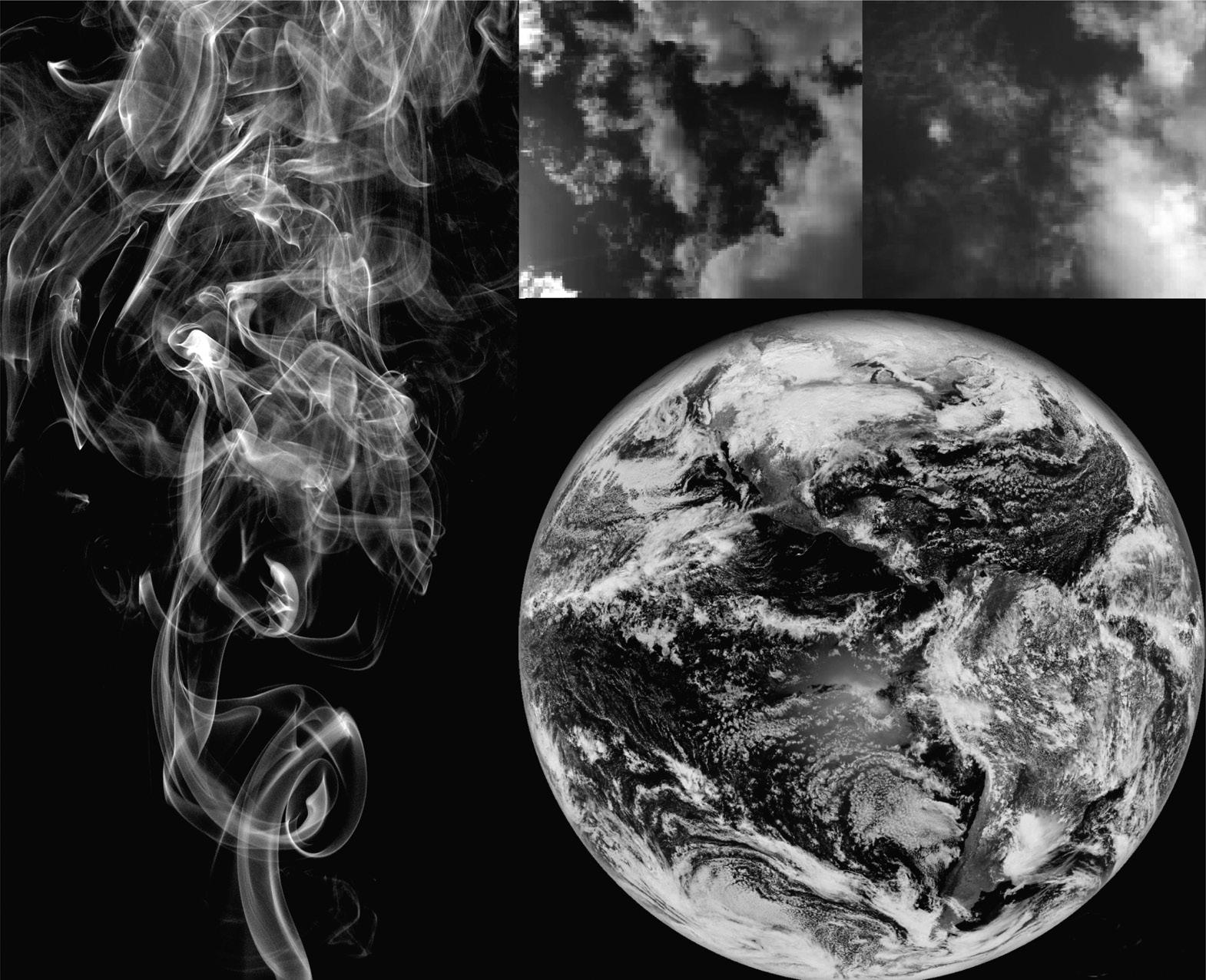
The key to answering these questions is the notion of scale, both in time (duration) and in space (size). Spatial variability is probably easier to grasp because structures of different sizes can be visualized readily (Fig. 1.1). In a puff of cigarette smoke, one can casually observe tiny wisps, whirls, and eddies. Looking out the window, we may see fluffy cumulus clouds with bumps and wiggles kilometers across. With a quick browse on the Internet, we can find satellite images of cloud patterns literally the size of the planet. Such visual inspection confirms that structures exist over a range of 10 billion or so: from 10,000 km down to less than 1 mm. At 0.1 mm, the atmosphere is like molasses; friction takes over and any whirls are quickly smoothed out. But even at this scale, matter is still “smooth.” To discern its granular, molecular nature, we would have to zoom in 1,000 times more to reach submicron scales. For weather and climate, the millimetric “dissipation scale” is thus a natural place to stop zooming, and the fact that it is still much larger than molecular scales indicates that, at this scale, we can safely discuss atmospheric properties without worrying about its molecular substructure.
a Often attributed to Mark Twain, but apparently it originally appeared much more recently in a science fiction novel by Heinlein, R. A. Time Enough for Love. (G. P. Putnam’s Sons, 1973).
Figure 1.1 (Left) Cigarette smoke showing wisps and filaments smaller than a millimeter up to about a meter in overall size. (Upper middle and right) Two cloud photographs taken from the roof of the McGill University physics building. Each cloud is several kilometers across, with resolutions of a meter or so.2 (Lower right) The global scale arrangement of clouds taken from an infrared satellite image of Earth, with a resolution of several kilometers.b Taken together, the three images of the clouds and Earth span a range of a factor of nearly a billion in spatial scale.
Clouds are highly complex objects. How should we deal with such apparent chaos? According to Greek mythology, at first there was only chaos; cosmos emerged later. Disorder and order are thus ancient themes of philosophy, physics, and . . . atmospheric science. In the case of clouds, their complex appearances are the result of turbulence. Turbulence arises when fluids are sufficiently stirred. Large-scale structures become unstable and break up into smaller ones. Neighboring structures can interact in complex ways. We can get a feel for this by putting a drop of milk in coffee. If you add the drop gently into a cup of calm black coffee, the milk diffuses very slowly. A brief, wide circular motion rapidly creates a homogeneous milky brew. Although the stirring only directly created a large
b The satellite picture was taken at infrared wavelengths. The colors are false. The whiteness depends on the coldness (and hence altitude) of the cloud top.
cup-size structure or whirl, it breaks up quickly, creating smaller and smaller ones that disperse the milk rapidly. When these eddies are a bit smaller than a millimeter, molecular diffusion takes over, making the mixture uniform. An important aspect of turbulence is that it typically leads to structures over huge ranges of scale, yet from the point of understanding the system, most of these structures are unimportant details. Rather than acquiring an understanding of each bump and wiggle, what we really need to understand are their statistics.
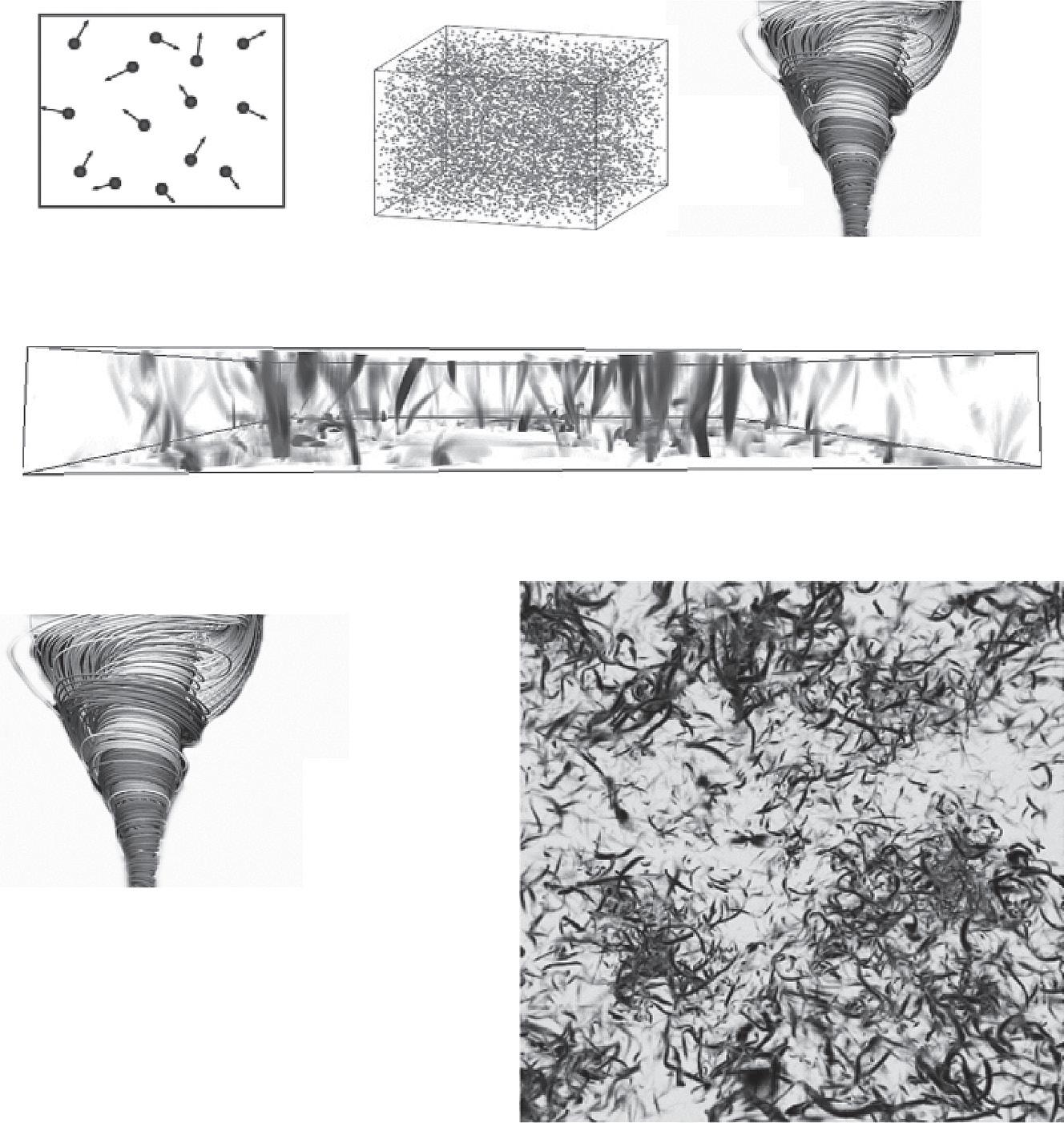
Cloud complexity is analogous to that encountered when considering matter at molecular scales. Figure 1.2A (left) shows a few molecules in a box. Classically, to understand the system at particle scales requires knowledge of the trajectories of each of the molecules.c Using a brute-force approach called molecular dynamics, today’s computers can handle such systems numerically with up to about a million molecules (Fig. 1.2A, middle), yet the systems are still tiny—a billionth of a nanogram or so. But describing and modeling matter at human scales is not just a question of computing power. It’s a conceptual problem. Here’s a mundane example: I heat my coffee and want to know what happens. Even if I knew the position and velocity of all of its million, billion, billion molecules, it would be mostly useless information. I would be happy with a single number: the temperature. Similarly, even if one could model every single eddy and structure in the atmosphere, every bump and wiggle on every cloud, it would still not answer the questions: Is it a nice day? Will it rain tomorrow? We need not only to eliminate the useless information, but also we must also use the appropriate concepts.
Fortunately, starting in the nineteenth century, techniques have evolved for dealing with huge numbers of molecules: statistical mechanics based on probabilities. If all we want are averages, then we may simplify even further and use thermodynamics and continuum mechanics. The latter theories were developed before the establishment of the atomic theory of matter and make no reference to its particulate nature. Although they treat matter as though it was a homogenous “continuum,” this assumption is nevertheless the basis of all theories and models of the weather and the climate. In the jargon of complexity science, they are emergent laws and their new concepts such as temperature and pressure are emergent properties. Figure 1.2A (right) shows a typical continuum mechanics simulation of an isolated vortex. Even if scientists could make a (lowlevel) molecular dynamics simulation of this vortex by describing each molecule, there would be no point. To understand it, we need a higher level description that averages out the unimportant molecular details.3 And although there may be no mathematically rigorous proof, it is widely accepted that there is no contradiction between the higher level continuum description and the lower level molecular one. Both are valid.
c A quantum mechanical description involves corresponding wave functions.
Mechanics of a few particles
Collective behavior of many particles: Statistical mechanics
Continuum mechanics of a single vortex
Collective behavior of many vortices: Turbulent laws
mechanics
Collective behavior of many particles: ermodynamics, continuum mechanics: A vortex
Figure 1.2 (A, left) A particle (molecule) depiction of a gas at molecular scales (nanometers). This is a classic “billiard ball”–type of description. A quantum description involves wave functions that determine the probability of finding the particles in different locations. (A, middle) At somewhat larger scales, we have hundreds of thousands of particles, and we may start to model the system using use statistical mechanics. (A, right) At macroscopic scales, perhaps tens of centimeters or larger, there are so many particles that we can average over the molecular fluctuations and use a continuum description. Here, we see a vortex.4 This level of description assumes the air is smooth, not granular (i.e., that it ignores its molecular nature). (B, top5) Many interacting vortices can still be handled computationally on the basis of continuum mechanics, but the evolution is complex and becomes difficult to understand in a simple mechanistic manner. Each elementary vortex (B, bottom left) is a bit like the molecules in (A, left). (B, bottom right) In this image, we are nearing the strong turbulence limit relevant in the atmosphere. Although this is still a supercomputer simulation, we can already see the problem of huge numbers of interacting vortices. As a result of the seemingly random collection of long, thin vortices, this turbulent view is sometimes called the “spaghetti” picture. This is a direct numerical simulation6 that models the smallest relevant scales explicitly. Numerical models of the atmosphere in general are only approximations; their smallest scales may be 10 km across. Implicitly, they average over large numbers of structures.
Continuum
of several vortices
But the atmosphere is not an isolated single vortex (Fig. 1.2B, bottom left) or even a manageably small collection of vortices (Fig. 1.2B, top). Rather, it is more like the turbulent “spaghetti plate” picture (Fig. 1.2B, bottom right) composed of huge numbers of vortices (eddies, structures). In the atmosphere, typical estimates of the number of interacting components—“degrees of freedom”—are a billion, billion, billion (1027), or about the same as the number of molecules in a cubic meter of air. Attempts to understand the corresponding statistics are at the origin of even higher level turbulent laws. Just as statistical mechanics treats large numbers of interacting particles and extracts the important aspects in the form of statistics, so do turbulent laws, which describe the collective behavior of huge numbers of interacting eddies (structures, vortices). Lewis Fry Richardson (1881–1953) proposed the first turbulent law during the 1920s. The saga of how it was finally vindicated in 2013 is told in Chapter 4. When Richardson’s law and others of the same type are suitably generalized, they describe the statistical properties of the atmosphere and climate over wide ranges of scales in space and in time. Just as continuum mechanics is a high-level law emergent with respect to the low-level (fundamental) laws of particles and statistical mechanics, the turbulent laws are high-level laws that are emergent with respect to those of continuum mechanics. Once again, the laws at different levels are believed to coexist, to be equally valid.d Just as the continuum laws allow new and unprecedented means for understanding, modeling, and forecasting a vortex, the same is true of the turbulent laws for large collections of vortices. Notice the alternation in Figure 1.2 as one moves up the scale from particle laws (deterministice ) to statistical mechanics (statistical), to continuum mechanics (deterministic), to turbulent laws (statistical, also called stochasticf ).
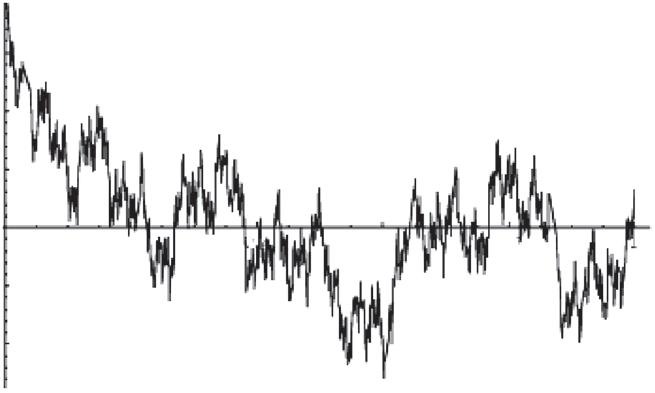
In practice, one chooses to use one description (level) or another, one model or another, depending on the application. The graphs in Figure 1.3 illustrate this. At the top, there is an actual wind trace, from measurements taken half a millisecond apart, that displays complex variability. This curve is from real-world data; it is neither random nor deterministic. These are attributes of theories and models. The scientist’s job is to find the theory and model that best fits reality, and to do this without a priori prejudices about whether it ought to be deterministic or stochastic7 (see Box 1.1).
d I say “believed” because, although there are many arguments and much evidence, there is no mathematical proof of the equivalence.
e This means that its evolution follows a rigid rule. This is the classical description. I could have started at the even more fundamental quantum level, which—being statistical—again alternates (see Box 1.1).
f Usually, the term statistical is used for descriptions of randomness, whereas the term stochastic is used for processes and models that incorporate randomness.
Figure 1.3 (Top) The trace of the wind speed on the roof of the McGill University physics building measured at 2 kHz (2,000 points over the 1 second of record that is shown). Note the detailed structure. The signal is still not smooth. (Lower left) Here there are 2,048 points of a stochastic (random) multifractal simulation with the same fluctuation exponent (H = 1/ 3) and measured multifractal parameters (see Box 2.2). (Lower right) Here, there are 2,048 points of a deterministic fractal model, the “Weierstrass function,”8 with the same fluctuation exponent (Section 2.3 and Box 2.3).
Box
1.1 Which chaos?
Order versus disorder and the scientific worldview
Although gods were traditionally invoked to explain cosmos and chaos (order and disorder), their role was drastically diminished with the advent of the Newtonian revolution. Sir Isaac Newton himself only required God’s assistance for the determination of the initial conditions—for example, starting the planets off in their orbits—the laws of mechanics and gravity would do the rest. By the middle of the nineteenth century, Newtonian laws had become highly abstract, whereas the corresponding scientific worldview had become determinism. The most extreme views have been attributed to Pierre-Simon Laplace (1749–1827), who went so far as to postulate a purely deterministic universe in which “if a sufficiently vast intelligence exists,”9 it could solve the equations of motion of all the constituent particles of the universe. In this universe, such a divine calculator could determine the past and future from the present in an abstract high-dimensional “phase space” that defines precisely the position and velocities of every particle and at all times.
Unfortunately, as part of their imperfect knowledge, mortals are saddled with measurement errors that involve notions of chance. The identification of chance with human error led to Voltaire’s (1694–1778) contemptuous: “chance is
nothing.” g By this, he meant that chance is purely subjective. As far as the laws of nature are concerned, it is beneath consideration. It was a full century later that James Clerk Maxwell (1831–1879) introduced probability explicitly into the formulation of physical laws: the distribution of speeds of gas molecules (in 1870). This is the origin of classic statistical mechanics—the idea that the unobserved or unknown degrees of freedom (“details”) are the source of random behavior, such as fluctuations about a mean temperature. Although highly partial information is the rule, human-size (macroscopic) objects are typically described by parameters such as temperature, pressure, and density. Most of the details—especially particle positions and velocities—are unimportant and can be reduced to various averages using statistics, hence the dichotomy of objective deterministic interactions of a large number of degrees of freedom coexisting with randomness arising from our subjective ignorance of the details.
The identification of statistics with ignorance evolved—notably thanks to Josiah Willard Gibbs (1839–1903) and Ludwig Boltzmann (1844–1906)—to the more objective identification of statistics with the irrelevance of most of the details. For example, Henri Poincaré (1854–1912) rejected the notion of chance as ignorance, and instead favored the view that chance is appropriate when dealing with complex causes. Giving the example of the weather and anticipating Edward Lorenz’s (1917–2008) Brazilian butterfly causing a Texas tornado, he stated: “It may happen that small differences in the initial conditions produce very great ones in the final phenomena. A small error in the former will result in an enormous error in the latter. Prediction becomes impossible and we have the fortuitous [chance] phenomenon.”h In Chapter 7, we see that this stochastic conclusion was more nuanced than Lorenz’s later deterministic one. A little later, Andrey Kolmogorov10 (1903–1987), perhaps motivated by fluid turbulence, “axiomatized” probability theory, proving that chance could be purely objective. This lent rigor to the work on Brownian motion initiated during the early twentieth century by Louis Bachelier, Albert Einstein, Marian Smoluchowski, and Paul Langevin. It laid the mathematical groundwork for dynamical stochastic processes that obeyed objective probabilistic laws.
But even these advances did not alter the deeply held prejudice that statistics and statistical laws were no more than a feeble substitute for determinism. A corollary to this was the hierarchical classification of scientific theories. Fundamental theories were deterministic; only the less fundamental ones involved randomness. Although this poor man’s view of randomness might have been appropriate to classic statistical physics, with its billiard ball atoms and molecules, it is incapable of accounting for the fact that the most fundamental physical theory yet devised—quantum mechanics—which is in fact probabilistic,11 with its fundamental object (the wave function) specifying probabilities.i Even today, although numerous developments make it obsolete, determinism is entrenched.
g He continues: “We have invented this word to express the known effect of unknown causes” (p. 439). Voltaire. The Ignorant Philosopher. (1766). (in English: Blue Ribbon Books, 1932.)
h Poincaré was a determinist. He was explaining why the weather “seemed” random; he was not arguing for a statistical theory of meteorology. Poincaré, H. Science and Method, p. 296. (Thomas Nelson and Sons, 1912).
i Not surprisingly, there have been attempts to explain quantum randomness by deterministic chaos acting at a subquantum level.
The deterministic chaos revolution: The butterfly effect
Just as biases toward determinism were starting to unravel, the deterministic chaos revolution of the 1970s and ʼ80s gave them a new lease on life. The trouble started with attempts to solve the equations of motion. Poincaré had already noted that three particles are already too many to allow for nice, regular “analytical” solutions. However, it was Lorenz, in 1963, who fully recognized the general propensity of nonlinear systems to amplify small perturbations (“sensitive dependence on initial conditions”)—a fact that only became widely known during the 1970s as the “butterfly effect” (see Chapter 7). Even if Laplace’s calculator had nearly perfect initial information and had infinitely precise numerics, the future would not be predictable. Randomlike “chaotic” behavior would result instead. During the 1950s, Lev Landau had proposed that fluid turbulence arose through an infinite series of instabilities. Now, thanks to Lorenz, it became clear—as the title of a famous article proclaimed12 that “three implies chaos.” However—and this crucial point is often overlooked—even if only three instabilities are necessary, the state of “fully developed fluid turbulence”13 that approximates the atmosphere still depends on a huge number of components.
To become a fully fledged revolution, in addition to the butterfly effect, chaos theory required two more developments. The first was the reduction of the scope of study to systems with a small number of degrees of freedom. The second was the discovery that, under quite general circumstances, qualitatively different dynamical systems could give rise to quantitatively identical behavior: the celebrated “Feigenbaum constant.”14 This “universality”15 finally allowed for quantitative empirical tests of the theory. By the early 1980s, these developments had led to what could properly be called the chaos revolution.
Later developments and problems
The basic outlook provoked by the developments in chaos—that randomlike behavior is “normal” and not pathological—is valid regardless of the number of degrees of freedom of the system in question. The success of chaos theory on systems with a small number of degrees of freedom led to some bold prognostications, such as “junk your old equations and look for guidance in clouds’ repeating patterns.”16
This fervor was unfortunately accompanied by a drastic restriction of the scope of chaos itself to meaning precisely deterministic systems with few degrees of freedom. The restriction, coupled with the development of new empirical techniques, led to a major focus on applications and a number of curious, if not absurd, claims.
A particularly striking example comes from the climate, for which it had always been assumed that a large (practically infinite) number of interacting components were involved. However, when new chaos tools were applied to paleoclimate data, a famous paper even claimed that only four degrees of freedom were required to specify the state of the climate.17 It was later pointed out that the conclusion was based on empirical analysis involving only 180 data points, and that even within the deterministic paradigm, this was far too few to justify the conclusions. It was barely noticed that, in any case, stochastic processes with an infinite number of degrees of freedom could have easily given the same result.18
During the same period, in geoscience and elsewhere, numerous attempts were made purely from data analysis to prove that, despite appearances, randomlike signals were in fact deterministic in origin.
These attempts were flawed at several levels, the most important of which is philosophical: the supposition that nature is (ontologically) either deterministic or random. In reality, the best that any empirical analysis could hope to demonstrate was that specific deterministic models fit the data better (or worse) than specific stochastic ones.
The alternative for large numbers of degrees of freedom: Stochastic chaos
By the mid 1980s, the ancient idea of chaos had thus taken on a narrow, restrictive meaning that essentially characterized deterministic systems with small numbers of interacting components. The philosophy underlying its use as a model for complex geophysical, astrophysical, ecological, or sociological systems—each involving nonlinearly interacting spatial structures or fields—has two related aspects, each of which is untenable. The first is the illogical inference that because deterministic systems can have randomlike behavior, randomlike systems are best modeled as deterministic. The second is that spatial structures that apparently involve huge variability and many degrees of freedom spanning wide ranges of scale can in fact be effectively reduced to a small number. At a philosophical level, deterministic chaos is a rearguard attempt to resurrect Newtonian determinism.j
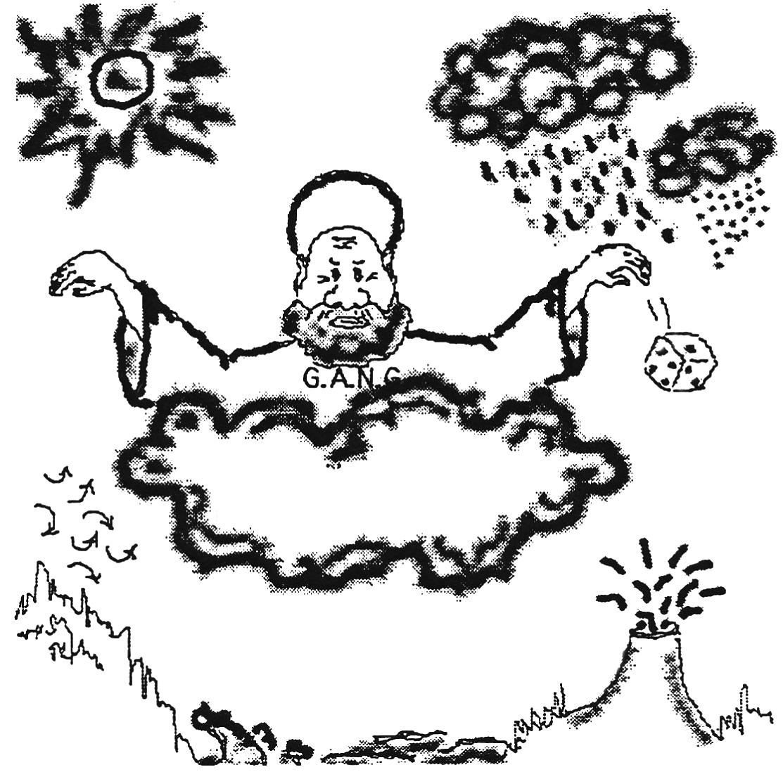
To overcome the limitations of deterministic modeling, I propose to make systematic use of models with objective randomness: “stochastic chaos.”19 The fundamental characteristic of stochastic theories and models that distinguishes them from their deterministic counterparts is that, mathematically, they are defined on probability spaces, which implicitly involve huge numbers of components.20 In comparison, their deterministic counterparts—at least when strongly nonlinear— are only manageable with small numbers of interacting components (degrees of freedom). The stochastic chaos alternative is now easy to state: Contrary to Einstein’s injunction that “God does not play dice,” we seek to determine how God plays dice with large numbers of interacting components (Fig. 1.4). Deterministic and stochastic models of the same physical system can coexist at different levels in a hierarchy of scientific theories. One can choose the level that is most convenient for the intended application.21
j In a popular book, the father of deterministic chaos, Edward Lorenz, even flirts with teleology— the idea that freewill is an illusion: “We must then wholeheartedly believe in free will. If free will is a reality, we shall have made the correct choice. If it is not, we shall still not have made an incorrect choice, because we shall not have made any choice at all, not having a free will to do so” (p. 160). Lorenz, E. The Essence of Chaos. (UCL Press, 1993).
Figure 1.4 God playing dice in geophysics. During the 1930s—the early days of quantum mechanics—Einstein famously proclaimed, “God does not play dice.” By this, he meant that, because of its stochastic nature, quantum mechanics could only be a provisional theory, and that it would be replaced eventually by a more fundamental, deterministic one. Today, quantum mechanics is still the most fundamental theory that we have, and the objective nature of such stochastic theories is much clearer than it was in Einstein’s day. Stochastic theories can be just as fundamental as deterministic ones. The modern question is: How does God play dice?22
Objections to stochastic chaos
Causality requires determinism
A common misconception is that causality and determinism are essentially identical or, equivalently, that indeterminism implies a degree of acausality. As emphasized by Bunge,23 causality is nothing more than a specific type of objective determination or necessity. It, by no means, exhausts the category of physical determination that includes other kinds of lawful production/interconnection, including statistical determination: stochastic causality.
Structures are evidence of determinism
Interesting phenomenologically identified large-scale structures—storms, for example—are frequently modeled with mechanistic (and deterministic) models, whereas the presence of variability without noteworthy structures is identified with noise. The inadequacy of this view of randomness is brought home by the still-littleknown fact that stochastic models can, in principle, explain the same phenomena. The key is a special kind of “stochastic chaos” involving a scale-invariant symmetry principle in which a basic (stochastic) cascade mechanism repeats scale after scale after scale, from large scales to small scales, eventually building up enormous
variability: multifractals (Box 2.2). Unlike classic stochastic processes, multifractals specifically have extreme events, called singularities, that are strong enough to create structures, so they produce potentially large structures that have little in common with featureless white noise.
Physical arguments for stochastic chaos: Turbulence
We have already seen that because stochastic processes are defined on infinite dimensional probability spaces, stochastic models are a priori the simplest whenever the number of degrees of freedom is large. In geoscience, stochastic chaos is particularly advantageous when—as in fluid turbulence—a nonclassic symmetry is present: scale invariance. This is the thesis of this book.
Consider the bottom graphs in Figure 1.3. On the left, we see a stochastic multifractal model with a basic fluctuation exponent (H; discussed in Chapter 2) that is close to the value found in the experimental trace at the top. In this case, it is close to a well-known theoretical turbulence law.24 On the right, we show a purely deterministic model with the same parameter, but it is based on a simple rule that repeats from large scales to small scales (a fractal). Although the left graph obeys high-level turbulent laws, the right might have comek from a (lower level, deterministic) Numerical Weather Model (NWP) or General Circulation Model (GCMl). Yet both could be realistic inasmuch as they agree on important statistical properties of the data. In this case, all three graphs in Figure 1.3 turn out to have the same basic relationship between large and small structures: the rule that determines how “fluctuations” change with size. In the data series (Fig. 1.3, top), the relationship can be determined by analysis; in the bottom (Fig. 1.3), the relationship is specified theoretically by the model. The idea is that the detailed wiggles (e.g., the curves in Fig. 1.3) are not of interest, but the way the wiggles typically differ when we move from small to large is of interest. Even in these model series, one may notice that their exact characters seem to be a little different. It turns out that the relation between small and large can itself be nontrivial, and a single number (in this case, the fluctuation exponent that we revisit in Chapter 2) is only part of the story.
Another way of viewing this is to ask: Do all the wiggles in Figure 1.3 (top) require detailed explanations? Or, when we consider enough wiggles over a wide range of scales, is there a simplifying principle that comes into play? If either of the bottom curves in Figure 1.3 were realistic wind models, the apparent wind
k Although, in this case, the finest resolution would be hours, not milliseconds!
l The acronym GCM refers to numerical models of the atmosphere that are adapted to timescales longer than the ten-day weather scale, notably by including a model of the ocean. Increasingly, the acronym GCM is alternatively decoded as Global Climate Model. Although GCMs are often distinguished from NWPs, their atmospheric components are fundamentally the same, being run on larger grids and with lower temporal resolutions. For the purposes of this book, the distinction is not always important.