Biogeochemical Cycles and Climate
Han Dolman
Vrije Universiteit Amsterdam
1Great Clarendon Street, Oxford, OX2 6DP, United Kingdom
Oxford University Press is a department of the University of Oxford. It furthers the University’s objective of excellence in research, scholarship, and education by publishing worldwide. Oxford is a registered trade mark of Oxford University Press in the UK and in certain other countries © Han Dolman 2019
The moral rights of the author have been asserted
First Edition published in 2019
Impression: 1
All rights reserved. No part of this publication may be reproduced, stored in a retrieval system, or transmitted, in any form or by any means, without the prior permission in writing of Oxford University Press, or as expressly permitted by law, by licence or under terms agreed with the appropriate reprographics rights organization. Enquiries concerning reproduction outside the scope of the above should be sent to the Rights Department, Oxford University Press, at the address above
You must not circulate this work in any other form and you must impose this same condition on any acquirer
Published in the United States of America by Oxford University Press 198 Madison Avenue, New York, NY 10016, United States of America
British Library Cataloguing in Publication Data Data available
Library of Congress Control Number: 2018960484
ISBN 978–0–19–877930–8
DOI: 10.1093/oso/9780198779308.001.0001
Printed and bound by CPI Group (UK) Ltd, Croydon, CR0 4YY
Links to third party websites are provided by Oxford in good faith and for information only. Oxford disclaims any responsibility for the materials contained in any third party website referenced in this work.
Preface
It was at the annual meeting of the European Geosciences Union in Vienna in 2014 that I was approached by Sonke Adlung from Oxford University Press with the question if any and, if so, what book was missing in my field of research. I think now that I did not immediately reply, but that it took me some time before I was able to clearly identify what was missing. The reasons for that lie in my experience of having taught Earth science students the basic physics of climate for some time, and in the fact that Earth science itself provides numerous beautiful examples of how that physics and biogeochemistry operated in the geological past, aspects which I did not teach. I needed some time to formulate the importance of presenting these together.
Most university courses present our students with a rather incomplete picture of the climate of our planet. Meteorology students are made familiar with the physics of the interaction of greenhouse gases and radiation, and the thermodynamics and transport of the atmosphere, but generally lack knowledge of the role of oceans and the interaction of the biosphere with climate. They also miss a palaeoclimatological perspective. Earth science students gain insight into long-term climate processes such as the geological thermostat, the role of plate tectonics in climate and various other aspects of palaeoclimate and biogeochemistry but are hardly made familiar with the physics of atmosphere and ocean.
The societal implications of this development are severe. We can only understand climate (change) as long as we can quantify the multitude of feedbacks between these important physical and biogeochemical and biological processes. This requires understanding not only what processes change the rates and magnitudes of biogeochemical cycles such as the carbon cycle, the nitrogen cycle and the water cycle but also how the physics of motion, thermodynamics and radiation respond to those changes.
This book follows from these considerations. It is about the science of the interactions and the exchange processes between reservoirs such as the ocean, the atmosphere, the geosphere and the biosphere. It is less about the human impact, as there is already a wealth of good textbooks that deal with issues of current climate change such as adaptation, mitigation and impacts. The book is primarily aimed at Earth science students who are at the advanced-bachelor’s or master’s level and have a basic understanding of algebra, chemistry and physics. Its purpose is not at all to be complete. It aims rather to provide a more integrated view of the climate system from an Earth science perspective. The choices of the subjects are, however, my own and based on personal and probably biased preferences. It is up to the reader to judge how well I succeeded in this complicated attempt at integration.
The first three chapters offer a general introduction to the context of the book, outlining the climate system as a complex interplay between biogeochemistry and physics
and describing the tools we have to understand climate: observations and models. They describe the basics of the system and the biogeochemical cycles. The second part consists of four chapters that describe the necessary physics of climate to understand the interaction of climate with biogeochemistry and change. The third part of the book deals with Earth’s (bio)geochemical cycles. These chapters treat the main reservoirs of Earth’s biogeochemical cycles—atmosphere, land and ocean—together with their role in the cycles of carbon, oxygen, nitrogen, iron, phosphorus, oxygen, sulphur and water and their interactions with climate. The final two chapters describe possible mitigation and adaptation actions, always with an emphasis on the biogeochemical aspects. I have tried to make these last six chapters as up to date as possible by providing more references in them than in the previous chapters.
I am grateful to Sonke Adlung for posing that initial question to me in 2014. He and Ania Wronski at Oxford University Press have always been very supportive of the project, even when the start was somewhat difficult. John Gash, former colleague and lifelong friend, edited the first draft. Various colleagues at the Department of Earth Science of the Vrije Universiteit have provided feedback, both on ideas and on chapters. Gerald Ganssen has always been a great stimulating force for this project and I very much appreciate his role as discussion partner providing the larger-scale geological perspective. I sincerely acknowledge the freedom I experienced in the Department of Earth Sciences to be able to write and finish this book as I wished. Further support was received from the Darwin Centre for Biogeology and the Netherlands Earth System Science Centre. Several people have commented on individual chapters: Antoon Meesters, Jan Willem Erisman, Joshua Dean, Sander Houweling Nick Schutgens, Appy Sluys and Jack Middelburg. Ingeborg Levin and Martin Heimann read the near-final draft. It is fully due to these people that several (embarrassing) errors have been corrected in time. I very much appreciate the opportunity provided by the president of the Nanjing University of Information Science and Technology and by Tiexi Chen and Guojie Wang to spend some time at Nanjing in the spring of 2018, that allowed me to finish the book. Kim Helmer was of great help in obtaining copyright permissions for the various figures used in this book.
The writing of this book took quite some time, but was overall a very enjoyable experience. I like to thank my lifelong partner Agnes and my two sons Jim and Wouter for their support. Words are simply not enough to express my gratitude to them.
Han Dolman
June 2018
4.1
8
5.4
6.1
6.2
6.3
6.4
6.5
6.6
6.7
8.1
8.2
8.3
8.4
8.5
9.5
9.7
9.8
9.9
9.11
Biogeochemical
cycles, rates and magnitudes
The movement of matter and transfer of energy around the planet plays a fundamental role in Earth’s system. It ensures that Earth is habitable and also determines the availability of key resources for human use. Take, for instance, the availability of fossil fuels such as the hydrocarbons oil and gas. The large-scale exploitation of these fossil fuel reserves has enabled Earth’s population to develop on an incredibly fast economic growth trajectory that has brought us great wealth and progress. However, the waste products of this fossil fuel use, primarily in the form of carbon dioxide and methane, are causing largescale perturbations in Earth’s climate. These have been assessed by the Intergovernmental Panel for Climate Change (IPCC) in a series of groundbreaking assessment reports, documenting rising sea levels, increasing temperatures, changing weather patterns, heatwaves and drought. In geological history, some of the greenhouse gases that are now playing havoc with the climate have played an essential role in regulating Earth’s temperature and created the conditions for life to evolve. At these long timescales, without human interference, the carbon atoms in carbon dioxide and methane molecules would be continuously recycled in Earth’s geological cycles. Variations in the rate of biogeochemical cycling are key to understanding past climate variability and today’s climate change.
The rate and magnitude of biogeochemical cycling also determine the availability of food for humans, as the large-scale application of artificial fertilizer shows. Haber invented the process for the industrial production of ammonia from atmospheric nitrogen in 1908; since then, many more people on Earth have been fed, particularly in the period after the Second World War. The concomitant population explosion has, however, happened at the cost of substantial changes to the biogeochemical cycle of nitrogen and to the environment, to the extent that now the nitrogen cycle is dominated by input from anthropogenic processes. Environmental effects include contamination and eutrophication of freshwater bodies, and excessive atmospheric deposition and emissions of a potent greenhouse gas, nitrous oxide.
The Russian scientist Vladimir Vernadsky is generally credited with defining the notion of the biosphere in his landmark 1926 book, the Biosphere and the associated biogeochemical cycling of material and energy within the biosphere (Vernadsky, 2012). In his view, the biosphere is one of Earth’s concentric envelopes, containing not only life
but also the minerals that are cycled through the activity of life and geological processes. He was the first to entertain the notion that the composition of the atmosphere was in some way regulated by life. One could argue that he identified living matter as a geological force in its own right, a concept that has now found its human equivalent in the modern concept of the Anthropocene (Crutzen, 2002).
The impact of biogeochemical cycles on climate and vice versa can conveniently be phrased as three questions:
• How have the cycles of key nutrients, such as carbon, nitrogen and phosphorus, and water changed, both in the geological past and, more recently, through the impact of humans on the Earth system?
• How do these cycles interact with each other and the physical properties of climate?
• How can we use this knowledge to mitigate some of the impacts of the changing biogeochemistry on climate, and Earth’s habitability and resilience?
This book is about these three aspects of biogeochemical cycling and Earth’s climate. Understanding the exchange of materials and its relation to climate is important, in particular if these exchanges involve radiatively active trace gases such as carbon dioxide, methane and nitrous oxide. Through their absorption characteristics in the infrared radiation domain, these trace gases directly interact with the climate.
While the geological forces that have shaped the environment over millions and billions of years impact the size and availability of fluxes and reservoirs, geology also provides key signature information on changes in biogeochemical cycles, through longterm records of the composition and abundance of specific minerals and isotopes in sediments and rocks. These records are not always straightforward or easy to interpret; however, the geological memory is an important asset in providing the larger picture of the interaction between biogeochemistry and climate. We will take this double-sided perspective in this book: Earth science is both our tool and our study object.
1.2 The geological cycle
One of the important characteristics of Earth is its continuous recycling of rocks, soils and material through what is known as the geological cycle. The geological cycle is traditionally described as a set of four related cycles: the tectonic cycle, the rock cycle, the hydrological cycle and the biogeochemical cycles. The last two figure prominently in this book. Virtually all of these cycles are, in some way, interlinked but they differ in the timescales at which key processes occur. The tectonic cycle involves the creation and destruction of the lithosphere (Earth’s outer layer, which is roughly 100 km deep) through a process called plate tectonics. Not all planets have this phenomenon, at present, it appears to be a unique feature of Earth. Planetary geologists still debate why Earth is the only planet in the solar system with active plate tectonics. Plate tectonics operates at timescales of tens of millions of years and involves the movement of large
The carbon cycle 3 plates on a substrate of denser material at speeds of 0.020–0.150 m yr−1 depending on the plate and geological period. On the one hand, the tectonic cycle involves the creation of new materials, or lithosphere, at oceanic ridges, in a process called ‘sea-floor spreading’. On the other hand, it involves the destruction of these in ‘subduction zones’, where an oceanic plate dives, or subducts, due to its larger density, beneath a lighter continental plate. Subduction zones are the places with the most active volcanoes and where seismic activity is strongest. Where tectonic plates of similar density meet, mountain ridges are produced as a result of the collision; the Himalayas and the Rocky Mountains are prime examples of this. Plate tectonics shapes the continents, oceans and mountain ridges of the planet, and has an important impact on climate—not least because the placement of continents affects the ocean circulation. Plate tectonics provides the critical recycling mechanism for materials in Earth’s crust.
Trace gases such as carbon dioxide and methane, but also water vapour, define the radiative properties of the atmosphere, keeping the global tropospheric temperature well above freezing. On Earth, water can exist in its frozen, liquid and vapour forms and this is a prerequisite for life as we know it. Carbon dioxide is only present in Earth’s atmosphere in small quantities, with its concentration typically expressed in parts per million. This is fundamentally different to our neighbouring planets Venus and Mars, which both have atmospheres comprising more than 95% carbon dioxide. It is estimated that, if there had not been life on Earth, its atmosphere would contain 98% carbon dioxide. The amount of carbon in Earth’s atmosphere is, however, marginal compared to the quantities of carbon locked up in the deep Earth, sediments and ocean reservoirs.
It is worth emphasizing these differences between the carbon stocks of the surface reservoirs and the stores of carbon in Earth’s core, mantle and continents. Earth’s core is estimated to contain 4 billion petagrams of carbon (Pg C; 1 Pg = 1015 grams), which is 90% of the total amount of Earth’s carbon, an enormous 1 million times more than the three surface reservoirs together (DePaolo, 2015). This deep carbon does not exchange with the other reservoirs but has probably played an important role in establishing climate on the very young Earth, some 4.5 billion years ago. Earth’s mantle contains about 240–400 million Pg C, roughly 8%–9% of the total amount of Earth’s carbon. This carbon appears as diamonds and impurities in minerals. About a quarter, 60–70 million Pg, of this is located in Earth’s crust, forming the continents and the ocean floor. Its main forms are limestone and dolomite, and its pressurized form is marble. This carbon may be released from the crust to the atmosphere through volcanism and geysers.
1.3 The carbon cycle
To illustrate the impact of biogeochemistry on climate, let us pay some further attention to the carbon cycle. The biggest game-changing event in Earth’s biogeochemical history was arguably the production of organic matter and oxygen by cyanobacteria, algae and green plants (Langmuir & Broecker, 2012). In the presence of solar radiation,
This equation is fundamental to our understanding of the carbon and oxygen cycle, past and present, and we will come back to it numerous times in this book. It describes the production of oxygen and sugars through oxygenic photosynthesis. The subsequent reverse process, respiration, consumes oxygen and sugars in an exothermic reaction. To a large extent, the balance of these two processes determines the size of surface reservoirs of carbon and oxygen. However, interactions with other geological processes, such as reactions with reduced materials from Earth’s crust (e.g. sulphur and iron) or the burial of organic matter, can take carbon temporarily out of the equation and shift the equilibrium towards the right, thus increasing the amount of oxygen. Of course, the opposite can also happen. That part of the carbon cycle where this equation plays the central role is named the organic carbon cycle (see Figure 1.1). We will see later that its importance in regulating climate depends on the timescale we look at and that it cannot explain all the variability of the geological record (see Chapter 9). For that, we also need to look at another part of the carbon cycle.
This other part, the inorganic carbon cycle, is often called Earth’s geological thermostat and is shown schematically in Figure 1.2. It describes how, in its solid form, calcium carbonate is in a subtle exchange process with carbon dioxide in the atmosphere. The rate of exchange between atmosphere, ocean and crust appears to control climate at million-year timescales. It is dependent—as the name suggests—on the geological cycle, but it is also dependent on the availability of liquid water in the hydrological cycle. Weathering of exposed rock surfaces, either physically, by freezing and cracking, or chemically, by dissolution, produces smaller particles of these rocks; these particles are then transported by wind, water or ice. When these materials collate together and sink to the floor of the ocean basins, sediments are produced. The weight of the new sediments
6H2O + 6CO2 ↔ C6H12O6 + 6O2
6H2O + 6CO2 ↔ C6H12O6 + 6O2
River transport
Sedimentation
Figure 1.1 The organic carbon cycle based on the conversion of carbon dioxide and water into oxygen and sugars (biomass). The speed at which the sediments are buried and subsequently returned to the atmosphere through subducting plates that emit volcanic carbon dioxide links the organic carbon cycle to the tectonic cycle.
Figure 1.2 The inorganic carbon cycle containing the geological thermostat. The speed at which the sediments are buried and subsequently returned to the atmosphere through subducting plates that emit volcanic carbon dioxide then determines the net long-term balance of carbon dioxide in the atmosphere.
carbon cycle 5 compacts the underlying layers further until sedimentary rocks are produced. These then enter the tectonic cycle and may be transformed by heat and pressure into metamorphic rocks or lifted up to the surface by plate tectonics, where a new cycle of weathering can start. The ocean, in particular the deep ocean, thus plays a key role in linking the fast and slow carbon cycles.
A closer look at the chemistry of water, carbon and the rocks of the inorganic carbon cycle shows the fundamental importance of this part of the carbon cycle on geological timescales (Langmuir & Broecker, 2012). Water falling on Earth’s land surface lets rocks and soil react chemically with the main minerals, calcium and silicate:
Equation (1.2a) shows how water and carbon dioxide act together to dissolve the calcium silicate (the mineral wollastonite) to produce calcium and carbonate ions and a silicate. In today’s ocean, calcium is used to form the shells of small unicellular and multicellular organisms that ultimately sink down to the ocean floor. In the absence of these organisms, the calcium and bicarbonate ions react to give calcium carbonate that then precipitates to the ocean floor (eqn (1.2b)).
The reason why these equations are so important in controlling Earth’s climate is that the dissolution of one molecule of wollastonite occurs at the cost of precisely one molecule of carbon dioxide (note that there are two molecules of carbon dioxide going in on the left side of eqn (1.2a) but only one coming out on the right side of eqn (1.2b)). This provides a mechanism for the effective removal of carbon dioxide from the
atmosphere by Earth’s crust. But this is not the full story: eqn (1a) also shows the importance of water. If there is more water, that is, in the form of precipitation, the weathering rate should go up and thus also the amount of carbon dioxide removed from the atmosphere. Higher temperatures can lead to increased precipitation by increasing the water-holding capacity of the atmosphere. If the atmospheric concentration of carbon dioxide increases, the temperature goes up and thus more carbon dioxide is removed. If the temperature goes down, the opposite happens, and the carbon dioxide concentration in the atmosphere, and the temperature, will go up. This feedback loop is thought to be the main regulator of Earth’s climate at geological timescales and shows how intricately water, the carbon cycle and climate are linked: the main thesis of this book. The fact that it operates at a geological timescale makes testing and finding hard evidence problematic, so it is best considered a (very) likely hypothesis (but see also Chapter 12).
The inorganic carbon cycle operates at timescales of millions to billions of years and is of little use to the current increase in carbon dioxide due to the use of fossil fuels. Indeed, on top of this slow inorganic cycle operates a much faster carbon cycle (Ciais et al., 2013). Here, fluxes of carbon involve the uptake of carbon by plants through photosynthesis, its subsequent respiration (eqn (1.1)) both on land and in the ocean, and the uptake of carbon dioxide by the ocean. The fluxes of this part of carbon cycle impact the surface stores of Earth, the carbon reservoirs of ocean, land and atmosphere. By far the largest amount of carbon is stored in the ocean, about 40,000 Pg C. The amount of carbon stored on land is tiny in comparison, a mere 500 Pg C in the biomass and 3–4 times that in the soil (pre-industrial numbers), with an additional 1,700 Pg C locked up in the soils of the permafrost areas, mostly in Siberia (see Chapter 10). In the atmosphere, the third exchange reservoir, the amount stored is comparable to that of biomass on land, about 500 Pg C.
Compare these minute amounts with those we mentioned earlier for the deep Earth and crust; they comprise a mere 1%–2% of the total carbon reserves of Earth. However, the carbon in the smallest of these, the atmospheric reservoir, and in concentrations of carbon dioxide in parts per million, provides the key to climate and how it changes in the short term. In the longer term, the oceans’ uptake capacity and their ability to transport carbon dioxide to their deeper layers, the ocean sediments, and, on a much longer scale, tectonic movements and volcanism are the important players.
1.4 Feedbacks and steady states
Feedbacks such as that of the geological thermostat, as well as from the burial of organic matter, play a crucial role in the complex system of Earth’s climate. A feedback either dampens or strengthens an original signal. Negative feedbacks stabilize a system; positive feedbacks amplify initial perturbations. For a feedback to occur, several components are needed: an initial signal, a process that responds to this signal, and an amplifying or dampening mechanism. A classic example in climate science is the ice–albedo feedback. Ice has a high albedo and thus reflects a large amount of sunlight, substantially more so than open water or land. The ice surface therefore stays cool relative to open water or land.
Feedbacks and steady states 7
If the temperature increases (the signal), more ice can melt (the process in the feedback loop). This results in more open water and ice-free land, and even higher temperatures, which cause even more ice to melt. This kind of feedback, where an initial signal is amplified over and over again, is a positive feedback loop. One example of a negative feedback is growing-season phenology: here, warmer temperatures extend the growing season, leading to more photosynthesis. The increased carbon drawdown can act to reduce the amount of warming. Here, the signal is the temperature of the atmosphere, the process is photosynthesis and the result is a dampening of the initial signal.
In a steady state, the size of the reservoir and the magnitude of the fluxes do not change. Cycles involving exchange fluxes between reservoirs are often depicted with a box model (Figure 1.3). The simplest cycle would involve two reservoirs, S1 and S2, between which fluxes are exchanged as F1,2 and, vice versa, F2,1. In steady state conditions, the following equation holds:
In practice, all (bio)geochemical cycles have components, or storage reservoirs, on land, in the ocean and in the atmosphere, thus adding a third reservoir to our simple box model. This adds complexity in the form of new exchange and return fluxes, as now six fluxes are important rather than two. It is difficult to generalize this, as adding new components generally involves exchanges with one or two of the other reservoirs only. The interplay between such a set of exchange fluxes determines the complexity and stability of a cycle, as feedbacks may be strengthened or weakened by changes in the size of the fluxes.
An important descriptor of the functioning of a cycle is the ratio between the size of the reservoir (i.e. the mass) and the flux. If the fluxes are small compared to the size of the reservoir, the process generally has little implication at short timescales. The reverse is true if the flux is large compared to the size of the reservoir. This ratio is called the turnover time. This is equivalent to the mean residence time under steady state conditions and represents the average time it takes for a molecule to pass through the reservoir (e.g. Bolin & Rodhe, 1973). The mean residence time, τ, is calculated as the ratio of the mass of the reservoir to the sum of either input or output fluxes and assumes steady state conditions:
Figure 1.3 Schematic drawing of a very simple geological cycle with two reservoirs and two reciprocal exchange fluxes
Table 1.1 The fluxes, reservoir sizes and calculated the mean residence time (τ) for key reservoirs of the carbon cycle. (Values from Ciais et al., 2013)
In Table 1.1 the magnitude of the fluxes and reservoirs of the carbon cycle are given and used to calculate the mean residence times, to indicate the stability of carbon in the reservoirs. As the sizes of the fluxes and the reservoirs are similar, the lowest mean residence times for carbon are obtained for the atmosphere and the vegetation. The ocean reservoir—given its enormous size—has a mean residence time for carbon of 500 years for a molecule of carbon dioxide. It is important to realize that, although the lifetime of an individual molecule of carbon dioxide in the atmosphere is relatively short, in most cases this simply implies that a molecule is taken up by the ocean and land, and another molecule swapped back. For the warming potential of carbon dioxide, the mean residence times of carbon in the reservoirs are thus less important than the absolute amounts. The processes ensuring the uptake of carbon by vegetation and ocean are critically important in determining the rate of change of the atmospheric carbon stock, and hence climate change. We can illustrate this further by showing the impact of mean residence times on the change of the size of the reservoirs after an initial pulse of carbon dioxide for the normalized change in atmospheric content since the industrial revolution. Figure 1.4 shows how the initial uptake takes place within the reservoir with the fastest response time, in this case, the land system (taken as the mean residence time for soils, from Table 1.1). We assume that
which shows that the rate of change in reservoir S, the atmosphere, in our case, is assumed to be proportional to a constant β times the size of the reservoir. The mean residence time is then the reciprocal of this constant. Note also that the mean residence time is equivalent to the time it takes to drop to 0.31S, that is, 1/e of the initial value S0 In this extremely simplified model, it would thus take the land about two hundred years to get rid of the assumed pulse of anthropogenic carbon dioxide, provided it continues to take up carbon. This is, of course, not quite realistic, because of the ultimately limited capacity of the biosphere to absorb carbon. So, the decline will be much less rapid and, importantly, feedbacks exist between the organic part of the carbon cycle and climate, through the temperature and moisture sensitivity of respiration and photosynthesis,
Figure 1.4 Removal of carbon dioxide, expressed as the fraction of carbon dioxide remaining in the reservoir after an initial pulse (100%) is fed through the main reservoirs: land, deep ocean and the carbonate system. The mean residence times used are based on the values given in Table 1.1 and a simple first-order differential equation in which the removal rate is set proportional to the size of the reservoir and the reciprocal of the mean residence time, that is, eqns (1.5a) and (1.5b).
which renders this rough calculation even less accurate. The deep ocean removes carbon at much longer timescales. At even longer, geological timescales, inorganic carbonate sedimentation moves carbon from the ocean into the crust: these processes would take several tens or hundreds of thousands of years to remove the pulse of human carbon dioxide. Over the first 500 years after the pulse, this system would only remove 1% of the initial pulse.
This model does not take into account the full buffering capacity of the ocean’s carbonate system. This may make the uptake of carbon considerable less than estimated here (see Chapter 9). Despite these caveats, the calculations make several important points. In the long term, Earth will recover from the pulse of fossil fuel emission humans have injected into the atmosphere, initially through the action of both the land and the oceans, and later primarily through the action of the larger reservoir, the ocean. However, limits exist to the uptake capacity and rate of these systems; for the oceans, this will be a very slow process. Interestingly, the uptake of carbon by land and ocean currently takes ‘care’ of about half our emissions, preventing a much stronger heating of the planet. We will explore this feedback in more detail in Chapters 9 and 13.
1.5 The greenhouse effect and the availability of water
After showing the importance of reservoirs and fluxes in responding to a change in input, let us go back to the role of greenhouse gases in climate. The physics of the greenhouse effect is dealt with in detail in Chapter 4 so, for the moment, a brief introduction will suffice. Gases, particularly those whose molecules comprise more than two atoms, such as carbon dioxide, nitrous oxide, water vapour and methane, have the ability to absorb radiation at specific wavelengths in the infrared domain of the electromagnetic spectrum, that is, wavelengths just longer than those of visible light. We call these gases ‘greenhouse gases’. However, they are also able to radiate this radiation back into all directions. So, if the atmosphere is warmed from below by radiation from Earth, the greenhouse gases in the lower atmosphere will absorb part of this radiation and radiate it back to Earth, effectively warming the lower atmosphere. The details of greenhouse gas radiation absorption and emission are undisputed and were discovered in the middle part of the nineteenth century by Fourier, Tyndall and Arrhenius. For now, it is sufficient for us to know that an increase in greenhouse gas concentrations will lead to an increase in temperature. How much exactly this increase is, and how much this impacts, for instance, the hydrological cycle and other processes on Earth, we can blissfully ignore for the moment. We will use this greenhouse effect of water vapour and carbon dioxide to explain how water vapour, liquid water and frozen water can coexist on Earth (e.g. Kasting, 2010). The availability of water in these three states is essential for life as we know it: too cold an atmosphere will yield only ice, while too hot an atmosphere will contain only water vapour. Let us assume that all of the three planets Venus, Earth and Mars started their lives as bodies without an atmosphere, at 0.72, 1.00 and 1.52 AU, respectively (AU = astronomical unit, the normalized distance of a planet from the Sun; Earth is, by definition, 1.00 AU from the Sun). Let us further assume that, at this stage, the geological cycle was organized in such a way that volcanoes emitted large quantities of water vapour and carbon dioxide. Now, water vapour, like carbon dioxide and methane, is a strong greenhouse gas, absorbing radiation in the infrared waveband. If there is enough water vapour and carbon dioxide to create a greenhouse effect, the planet’s surface temperature will increase. It is however also important to appreciate some of the peculiarities of water. The saturation water vapour pressure is the amount of water the atmosphere can hold before water starts to condense and this is a strong function of temperature. The exact relation specifying this, the Clausius–Clapeyron equation, is exponential in shape: the hotter the atmosphere, the more water the atmosphere can hold (see also Chapter 6). On Earth, for every degree of temperature increase, the atmosphere can hold 7% more water vapour. In the case of Mars, at 1.52 AU from the Sun, the starting temperature would have been low, around 220 K. Once the atmosphere contained enough water to start condensing out to ice (around 2 Pa), it would lose all the water to ice. This is shown in Figure 1.5 as the intersection between the Mars curve and the ice saturation curve. This confirms to a large extent what we currently see on Mars—a frozen desert with a thin atmosphere. In contrast, on Earth, starting at a higher temperature of around 270 K, only 3 K below the freezing point, water could accumulate in the atmosphere at a much higher concentration before it started to condense. The slight upward trend indicates a greenhouse
Figure 1.5 Schematic drawing showing the runaway greenhouse effect on Venus, whereas Mars remains an ice-frozen planet, and Earth is able to hold water in its three forms. (After Kasting, 2010)
effect caused by the water in the atmosphere. The main result is that the surface temperature increased above 273 K, allowing liquid water first to evaporate and later to condense higher in the atmosphere, where it would be colder. With virtually all water now located in the oceans, evaporation produces the counter flux, initiating a hydrological cycle on Earth. But what happened to Venus?
Venus started off warmer, at around 315 K, because of its proximity to the Sun (0.72 AU). This allowed large amounts of water vapour to accumulate in the atmosphere, but on Venus saturation was never reached. At some point, the curve goes sharply upwards and it never intersects with the saturation curve of water, as in Mars (ice) or on Earth (liquid). This is why we speak of a runaway greenhouse effect on early Venus. There are considerable simplifications in the precise application of these calculations but, by and large, they would probably have led early Venus to have a very hot and steamy atmosphere. But, without a hydrological cycle, at later stages all this water would have been lost through photodissociation (the dissolution of water into hydrogen and oxygen atoms, where the hydrogen atoms are lost to space because of their low atomic weight), leaving a hot and dry planet. On this planet, the weathering part of the long carbon cycle would have been slow, due to the absence of precipitation and because carbon dioxide emitted from volcanoes was allowed to remain in the atmosphere. There is estimated to be as much carbon dioxide in Venus’s atmosphere as there is in all of Earth’s carbonate rock formations.
1.6 The rise of oxygen
What happened on Earth after the temperature began to stabilize? At some point, oxygen came into the picture. The rise of atmospheric oxygen to its present-day concentration
of 21% by volume serves as another good illustration of how intricately biogeochemical cycles, such as those of oxygen and carbon, interact with the geological forces and cycles of the planet. Oxygenation of the planet involves oxygenation of the main reservoirs: Earth’s crust, the oceans and the atmosphere. It is commonly accepted that around 2.1 and 2.4 Gyr (1 Gyr = 109 years) ago, the concentration of oxygen began to rise from a minor 0.001% to its current value. This change is known as the Great Oxidation Event. However, as the range in timing already suggests, this is unlikely to have been a single big event. It is, for instance, not quite clear at precisely what time oxygen-producing bacteria entered the early planet’s stage. Recent evidence suggests that this may have happened well before 3 Gyr ago. However, the current oxygenation of the deep ocean is thought not to have been fully completed until about 600 million years ago, leaving about 2 Ga to complete the oxygenation on Earth through a multitude of interactions with other biogeochemical and geological cycles.
Two chemical species play a major role in tracking the rise of oxygen on the planet: iron and sulphur. We will come back to them in Chapter 12. Their evolution is a perfect example of how geological records help us to understand Earth’s biogeochemistry (Langmuir & Broecker, 2012). Today’s rocks and oceans contain abundant quantities of oxidized iron and sulphur, in the forms of Fe3+ and S6+, respectively. The oxidized form of iron, ferric iron, is non-soluble in water, whereas the reduced form, ferrous iron, is easily soluble. In contrast, sulphur’s oxidized form, sulphate, is highly soluble in water, while the reduced form, sulphite, is not. This behaviour can thus be used to track Earth’s oxygenation state, as the ratio of iron to sulphur in rocks indicates the level of oxygenation. An Earth with low oxygen content would appear reduced and would contain little sulphite in the oceans and large amounts of ferrous iron. Importantly, in an atmosphere containing substantial amounts of oxygen, any ferrous material exposed through weathering would become quickly oxidized and thereby lose its solubility in water. Today’s oceans are thus deficient in iron, whereas current day soils, in contrast, contain more iron than older soils (>2.4 Gyr ago). This deficiency in seawater has led to a series of grand experiments to fertilize the ocean with iron to improve carbon uptake. We will come back to some of these geoengineering ideas and experiments in the final chapter (Chapter 13).
Burial of carbon can take organic carbon temporally out of the cycle, thereby shifting eqn (1.1) towards the right and so increasing the amount of free oxygen. The fraction of organic material buried, however, has remained remarkably constant over Earth’s history (see Chapter 9 for more details). Nevertheless, through the use of isotopes (Chapter 3), it has been established that, around 2.0 –2.4 Gyr ago, much larger amounts of organic matter were buried. This may have led to an increased availability of oxygen. Exactly how this happened is largely unknown.
It is now assumed that the first photosynthetic bacteria appeared around 3 Ga ago. These would have produced whiffs of oxygen in an otherwise low-oxygen-content atmosphere; these are visible in the record in the early period from 2.5–3.0 Gyr ago. After this time, atmospheric levels rose, but it then took almost 2 Gyr to completely oxidize the ocean. This long time span is related to the vast size of the reservoir and the long residence times. The rates of oxygenation of Earth’s ocean and atmosphere are important to understand, as they indicate the sensitivity and vulnerability to changes.
For oxygen we noted that substantial changes in these rates have occurred over Earth’s history. There is an interesting corollary with climate in this story, relating to the fact that, before the oxygenation, the atmosphere probably contained large amounts of the strong greenhouse gas methane. The rise of oxygen could have oxidized this methane, resulting in a much cooler environment and starting off one of the great Snowball Earth episodes, just over 2.5 Gyr ago. However, issues about the timing and the strength of this feedback are still unresolved. Complete coverage in ice changes the reflectivity (albedo) of Earth in such a way that, how the planet escaped from this Snowball Earth episode and became warmer, is still very much an unresolved issue. It is also thought that greenhouse gases played an important role in stabilizing Earth’s climate when the Sun had a much lower (70% of today’s) luminosity. Without these radiative effects of greenhouse gases, Earth could have easily fallen into a much colder equilibrium (see also Chapter 10).
1.7 Non-linearity
One of the most pervasive aspects of climates and biogeochemical cycles is the nonlinear behaviour of the system. Linear systems are relatively easy to understand. The reservoir analysis of mean residence time is essentially a linear problem: the flux scales linearly with the size of the reservoir (see eqn (1.4)). Furthermore, if the input changes by, say, a factor of 2, the output also changes by a factor of 2. Linear systems can be superposed: the behaviour of the systems is exactly equal to the behaviour of the sum of the parts. Non-linear systems are much harder to understand, and predicting the effects of small changes in one or two variables often requires full numerical simulation. Since Earth’s biogeochemical reservoirs interact with each other, where output from one reservoir becomes input to another, each reservoir, however small, has the capacity to affect the behaviour of the whole. This crosstalk between subsystems leads to a disproportional relationship between input and output: the overall system is non-linear, and effects cannot simply be superposed. Non-linearity gives rise to unexpected events, such as abrupt transitions across thresholds; unexpected oscillations, where the frequency of the output is not equal to that of the input signal; and chaotic behaviour. Chaotic behaviour exhibits sensitivity to the initial conditions, as was established in weather forecast modelling by one of its founders, Edward Lorenz. Tiny differences in initial states can expand and even explode into large differences in later states. Importantly, the values of these variables do remain confined to fixed boundaries, while never exactly repeating the same trajectory. The Lorenz butterfly is the iconic image of this type of behaviour.
Earth system models are our current tools for understanding the non-linear interactions between climate and the biogeochemical cycles (see Chapter 3). Because of the non-linearity, they solve fundamental transport and conservation equations on a three-dimensional model grid, using large ensembles of model runs with tiny changes in initial conditions.
One final consequence of non-linearity needs to be discussed here: emergent behaviour. The climate system is not only chaotic but also complex, in the sense that myriads of interactions between its subsystems can lead to emergent behaviour that is only visible and understandable at the scale and level above the subsystems. Chaos and emergence
Figure 1.6 Schematic drawing of possible stable and unstable states in a two-equilibrium system. The forcing factor (e.g. precipitation) is on the horizontal axis; the state variable (e.g. vegetation) is on the vertical axis. In this case, the stable states might be low-density desert vegetation (e.g. savanna) on the left, and a densely vegetated state (e.g. forest) on the right. In the unstable area, the system always moves into one of the two equilibrium states.
are the two sides of the coin of complex non-linear behaviour. Figure 1.6 shows a generic example of a non-linear system. The system has two stable states, and an area in the middle where the system is unstable and moves to either one of the preferred states. Examples of this type of behaviour can be found in the vegetation of the Sahara–Sahel system, where the system moves between a desert and dense vegetation, depending on the rainfall. Another classic example is the Snowball Earth state we encountered earlier, at the beginning of Earth’s oxygenation. Here, the stable states would represent an Earth covered in ice and snow, and a completely ice-free Earth, while the vertical axis would represent the energy leaving the planet. It is important to understand that, in this case, the feedback in the system works through the reflectivity dependence on temperature. Low temperatures create large reflectivities through snow and ice, while higher temperatures create low reflectivity through the absorption of solar radiation by vegetation. Another example may be Earth’s oxygenation, as described earlier: either the planet is in a stable state with a considerable amount of oxygen (21%), which would be comparable to today’s value, or it is in a stable state with a very low value of oxygen (0.001%). Feedbacks are thus key to the stability of the Earth system, and we will encounter many of them in the remaining chapters in this book.
The next two chapters offer a general introduction to the context of the book, outlining the variability of climate system as a complex interplay between biogeochemistry and physics and describing some of the tools we have to understand climate: observation
Forcing variable
Stable Unstable
Non-linearity 15 and models. The second part of the book consists of four chapters that introduce the climate physics necessary for understanding the interaction of climate with biogeochemistry, and climate change. These deal with radiation physics and the greenhouse effects, aerosols and the physics and dynamics of the atmosphere and the ocean. The third part of the book deals with Earth’s (bio)geochemical cycles. These chapters treat the main biogeochemical cycles found on Earth: the carbon, methane, nitrogen, phosphorus, iron, sulphur and water cycles and their interactions with climate. The final two chapters bring this knowledge together to describe climate in the future and possible mitigation and adaptation actions—always with an emphasis on the interaction between biogeochemistry and climate.
2 Climate Variability, Climate Change and Earth System Sensitivity
2.1 Earth system sensitivity
This chapter is about climate, climate change and climate variability. It also deals with the sensitivity of the Earth system to changes in its forcing parameters, particularly to changes in the biogeochemical cycles. This is a story of timescales, of changing boundary or forcing conditions and of the amplification or diminishment of key processes through the operation of Earth system feedbacks.
The glossary of the American Meteorological Society defines climate as ‘the slowly varying aspects of the atmosphere–hydrosphere–land surface system’, it goes on to say that
it is typically characterized in terms of suitable averages of the climate system over periods of a month or more, taking into consideration the variability in time of these averaged quantities. Climatic classifications include the spatial variation of these timeaveraged variables. Beginning with the view of local climate as little more than the annual course of long-term averages of surface temperature and precipitation, the concept of climate has broadened and evolved in recent decades in response to the increased understanding of the underlying processes that determine climate and its variability. (American Meteorological Society, 2019)
Climate can also be more loosely defined as the state of the climate system, where the climate system is composed of the lithosphere, the hydrosphere, the biosphere, the atmosphere, the cryosphere and, increasingly, the anthroposphere, the human component. This wider definition also includes the dynamics and exchange of material between these spheres, through the biogeochemical cycles and their interactions—for instance, the dynamics of ice sheets. For our purposes, it is important to recognize that the state of the biogeochemical cycles is thus an integral part of the climate.
Earth is 4.54 (± 0.05) billion years old. During its lifetime, conditions both within Earth and on its surface, as well as its climate, have changed remarkably. It is important to identify the timescales and the resulting rates at which some of these changes have
Year s Decades
Clouds, water vapour, lapse rate, snow/sea ice
Upper ocean
Timescale
Centur iesMillennia
Multi-millennia // Myr
CH4 CH4 (major gas-hydrate feedback; for example, PETM)
Vegetation
Dust/aerosol
Dust (vegetation mediated)
Entire oceans
Land ice sheets
Carbon cycle
Weathering
Plate tectonics
Biolog ical evolution of vegetation types
Figure 2.1 Timescales of processes in the climate system that determine variability and feedbacks. (After Rohling et al., 2012)
happened. Figure 2.1 shows some of the key processes determining the variability of climate (Rohling et al., 2012). Processes that are important at a million-year (106 year) timescale, such as tectonic processes, shown on the right-hand side of the diagram, can be considered constant at the much shorter timescales shown on the left-hand side of the diagram, as their boundary conditions do not change under shorter timescales. We have already encountered in Chapter 1 the importance of some of the slow processes, such as the geological thermostat, which involves interactions between weathering and the hydrological and geological carbon cycles. Our current climate change problem has a scale of a few centuries, essentially the time since humans started using fossil fuels. On multi-millennia to million-year timescales, the periodicity of the Pleistocene glacial–interglacial cycle is dominant.
Climate variability is defined by the World Meteorological Organization (WMO) ‘as variations in the mean state and other statistics of the climate on all temporal and spatial scales, beyond individual weather events’ (World Meteorological Organization, 2017). We can express the instantaneous value of a particular variable, say temperature, as the sum of a mean and a fluctuating part:
in which T is the average value of the variable over a sufficiently long time period (sometimes taken as thirty years but, on scales of geological interest, it can be much longer), and T ′ is the perturbation or variation from that mean. In the case of temperature, the perturbation would be the deviation from the mean, where the mean would be derived from the temperatures over the last thirty years at a particular location. The resulting T value would be the temperature on a specific day. Any climate variable can be decomposed in this way if the time series is long enough to obtain statistically relevant values. In fact, if we take a lumped approach and consider several variables, such as temperature, humidity, pressure and precipitation, together in some way, all the values on the left-hand side of the equation would represent today’s weather. The set of mean values would represent climate. Importantly, climate has always been variable and always will be variable.
Climate change, such as we experience now, or in the geological past, is a change in the mean state of the variable in eqn (2.1). This can be due to a variety of factors that we will explore in later chapters of this book. The difference between changes in the mean and those in the fluctuating part of eqn (2.1) is crucial, and finding ways to separate the two and identify forcing as opposed to internal variability is a key subject in climate science: it underlies for instance, the question of whether it is possible to attribute extreme weather events to human-made climate change.
2.2 Geological-scale variability
Let us first take a look at an example of geological-scale variability, to illustrate some key features of climate variability. In Figure 2.2, data from sediment cores taken at the ocean bottom are used to reconstruct deep-ocean temperatures (Zachos, 2008). The study used oxygen isotopes as a proxy for temperature; the technique of using these isotopes is explained in more detail in Chapter 3. For a precise explanation of the geological epochs, see http://www.stratigraphy.org/index.php/ics-chart-timescale. Figure 2.2 shows that, for the past 66 million years, the ocean temperatures have been dropping: the longterm temperature trend in the Cenozoic, comprising the periods from Palaeocene to Pliocene, is thus downward. This is a change in the mean value. However, superimposed on this trend is a large variability, as indicated by the spikes. These upward spikes are called hyper-thermals. Examples are the early Eocene Climatic Optimum (56 Myr ago) and the Palaeocene–Eocene Thermal Maximum (42 Myr ago). The latter transition is thought to have caused a global warming of 5 ºC. Understanding this rise in temperature and its interaction with the suggested large increase in carbon dioxide is a very active research area, since this may provide insight into how the Earth system deals with large injections of carbon dioxide into the atmosphere and may shed light on Earth’s current situation. A recent estimate puts the emission of carbon dioxide during this period at about 10% of our current emissions from fossil fuel burning (~10 Pg C yr 1) but over a much longer time period of 4000 years (Zeebe et al., 2016). We will further explore the Palaeocene–Eocene Thermal Maximum in Chapter 9.
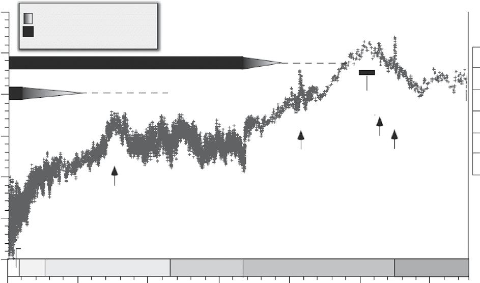
Figure 2.2 δ18O variability in ocean sediments over geological time. The δ18O variability is a proxy for temperature shown on the right axis; ETM1, Eocene Thermal Maximum 1; ETM2, Eocene Thermal Maximum 2; PETM, Palaeocene–Eocene Thermal Maximum. (After Zachos et al., 2008)
Most of the Cenozoic temperature variability appears related to carbon dioxide, coming from tectonic or volcanic origins. For instance, the rise around 60–50 Myr ago appears to be caused by the subduction of the carbonate crust from the Indian subcontinent, as this led to volcanic emissions that raised the carbon dioxide levels above 1000 ppm. In later stages, the concentrations of carbon dioxide declined, as the Indian and Atlantic oceans became sinks for carbon dioxide, and tectonic activity declined. Figure 2.2 also reveals the large variability in temperature during the Pliocene and Pleistocene, the period when Earth experienced glacials and interglacials. Overall, one can argue that the temperature trend suggests that Earth was slowly moving from a tropical greenhouse into a refrigerator world. The occurrence of ice sheets also appears to indicate this. These examples show that determining the average in eqn (2.1) clearly depends on the chosen timescale of interest (see Figure 2.1).
2.3 Glacial–interglacial variability
A palaeoclimatological proxy is a measurable quantity, such as tree rings, fossil pollen, ocean sediments, coral, the composition of trapped atmosphere in ice cores, and historical data that allows reconstruction of climate variability. Figure 2.2 shows that the δ18O variability in ocean sediments was large in the Pliocene. However, the interpretation