Instant Download Chi-squared data analysis and model testing for beginners 1st edition carey witkov
Chi-Squared
Visit to download the full and correct content document: https://ebookmass.com/product/chi-squared-data-analysis-and-model-testing-for-begi nners-1st-edition-carey-witkov/
More products digital (pdf, epub, mobi) instant download maybe you interests ...
Accelerated Life Testing of One-shot Devices: Data Collection and Analysis Narayanaswamy Balakrishnan
All rights reserved. No part ofthis publication may be reproduced,stored in a retrieval system, or transmitted, in any form or by any means, without the prior permission in writing of Oxford University Press, or as expressly permitted by law, by licence or under terms agreed with the appropriate reprographics rights organization. Enquiries concerning reproduction outside the scope ofthe above should be sent to the Rights Department, Oxford University Press, at the address above
You must notcirculate this work in any other form and you must impose this same condition on any acquirer
Published in the United States ofAmerica by Oxford University Press 198 Madison Avenue, New York, NY 10016, United States ofAmerica
British Library Cataloguing in Publication Data
Data available
Library of Congress Control Number: 2019941497
ISBN 978-0-19-884714 4 (hbk.)
ISBN 978-0-19-884715-1 (pbk.)
DOI: 10.1093/0s0/9780198847144.001.0001
Printed and bound by CPI Group (UK) Ltd, Croydon, CRO 4YY
Linksto third party websites are provided by Oxford in good faith and for information only. Oxford disclaims any responsibility for the materials contained in any third party website referenced in this work.
Preface
Recent ground-breaking discoveries in physics, including the discovery of the Higgs boson and gravitational waves, relied on methodsthat included chi-squared analysis and modeltesting. Chi-squared Analysis and Model Testingfor Beginners is the first textbook devoted exclusively to this method at the undergraduate level. Long considered a secret weapon in the particle physics community, chisquared analysis and model testing improves upon popular (and centuries old) curvefitting and model testing methods whenever measurementuncertainties and a model are available.
The authors teach chi-squared analysis and model testing as the core methodology in Harvard University s innovative introductory physics lab courses. This textbook is a greatly expanded version of the chi-squared instruction in these courses, providing students with an authentic scientist s experience oftesting and revising models.
Over the past several years, we ve streamlined the pedagogy of teaching chi-squared and model testing and have packaged it into an integrated,selfcontained methodology that is accessible to undergraduates yet rigorous enough for researchers. Specifically, this book teaches students and researchers how to use chi-squared analysis to:
¢ obtain the best fit model parameter values;
* test ifthe best fit is a goodfit;
¢ obtain uncertainties on best fit parameter values;
¢ use additional modeltesting criteria;
¢ test whether modelrevisions improvethefit.
Why learn chi-squared analysis and model testing? This book provides a detailed answerto this question, but in a nutshell:
In the old days it was not uncommon (though mistaken even then) for students and teachers to eyeball data points, draw a line of best fit, and form an opinion abouthowgoodthefitwas. Withthe advent ofcheap scientific calculators, Legendre s and Gauss s 200 year old methodofordinaryleastsquares curvefitting became available to the masses. Graphical calculators and spreadsheets made curve fitting to a line (linear regression) and other functionsfeasible for anyone with data.
Althoughthis newly popular form ofcurve fitting was a dramatic improvement over eyeballing, there remained a fundamental inadequacy. Thescientific method is the testing and revising of models. Science students should be taught how to
test models, not just fit points to a best fit line. Since models can t be tested withoutassessing measurement uncertainties and ordinaryleastsquares andlinear regression don taccountforuncertainties, one wondersifmaybe they rethe wrong tools for the job.
The right tool for the job of doing science is chi-squared analysis, an outgrowth of Pearson s chi-square testing of discrete models. In science, the only things that are real are the measurements, andit is the job of the experimental scientist to communicate to others the results oftheir measurements. Chi-squared analysis emerges naturally from the principle of maximumlikelihood estimation as the correct way to use multiple measurements with Gaussian uncertainties to estimate model parameter values and their uncertainties. As the central limit theorem ensures Gaussian measurementuncertainties for conditions found in a wide range of physical measurements, including those commonly encountered in introductory physics laboratory experiments, beginning physics students and students in other physical sciences should learn to use chi-squared analysis and model testing.
Chi-squared analysis is computation-intensive and would not have been practical until recently. A unique feature of this book is a set of easy-to-use, lab-tested, computer scripts for performing chi-squared analysis and model testing. MATLAB® and Python scripts are given in the Appendices. Scripts in computer languages including MATLAB, Python, Octave, and Perl can be accessed at HYPERLINK https://urldefense.proofpoint.com/v2/url?u=http3A__www.oup.co.uk_companion_chi-2Dsquared2020&d=DwMFAg&c=WORGvefibhHBZq3fL85hQ&r=T6Yii733Afo_ku3s_Qmf9XTMFGvqD_VBKcN4 fEIAbDL4&m=Q09HDomceY3L7G_2mQXKk3T9K1Tm_232yEpwBzpfoNP4 &s=DFO05tbd6j37MCerXNmVwfVLRSpA7pXaEx29lhsfBak4&e="www.oup.co. uk/companion/chi-squared2020.
Anotheruniquefeature ofthis bookis thatsolutionsto all problemsare included in an appendix, making the booksuitable for self-study.
We hope that after reading this book you too will use chi-squared analysis to test your models and communicate the results ofyour measurements!
MATLAB®js a registered trademark ofThe MathWorks, Inc. For MATLAB® productinformation, please contact:
All textbook authors owe debts to many people, from teachers to supporters.
The innovative Harvard introductory physics lab course sequence, Principles of Scientific Inquiry (PSI lab), that trains undergraduate students to thinklike scientists using chi-squared model testing, was innovated by physics professors Amir Yacoby and Melissa Franklin more than a decade ago. Important early contributions to PSI lab were also made byinstructors and instructional physics lab staff Robert Hart, Logan McCarty, Joon Pahk, and Joe Peidle. Both authors have the pleasure each semester of teaching PSI lab courses with Professors Yacoby and Bob Westervelt, Director ofHarvard s Center for Nanoscale Systems. We also gratefully acknowledge the helpful feedback provided by our many students, undergraduate Classroom Assistants and graduate Teaching Fellows over the years.
We are indebted to colleagues for reviewing this book and making valuable suggestions, including Bob Westervelt. Special thanks go to Preceptor Anna Klales, Instructional Physics Lab ManagerJoe Peidle, and Lecturer on Physics and Associate Director of Undergraduate Studies David Morin, who made detailed suggestions (nearly all ofwhich were adopted) for every chapter.
The authors, while thanking many people above for their contributions and feedback, blame no one but themselves for any errors and/or omissions.
Below are someauthor-specific acknowledgements.
CW: I thought I understood chi-squared analysis and model testing until I met Keith Zengel. Keith s willingness to share his in-depth understanding of the technicalities of chi-squared analysis and model testing over the past three years we ve taught together is greatly appreciated and gratefully acknowledged. I'd like to thank my 12-year-old son Benjamin (who decided sometime during the writing ofthis bookthathe doesn twantto be a physicist!) fornotcomplaining (too much) over time lost together while this book was being written.
KZ: I used chi-squared analysis a lot of times as a graduate student at the ATLASExperimentwithoutreallyunderstandingwhatI was doing.Later,I had to do a lot ofsecretive independent research to be able to answer the good questions posed by CareyWitkovwhenwestartedteachingittogether.I thinkwe managedto learn a good amountaboutthe subjecttogether, mostly motivated by his curiosity, and I hopethat others will benefitfrom Carey s vision ofscience education, where students learn how to speak clearly on behalfoftheir data.
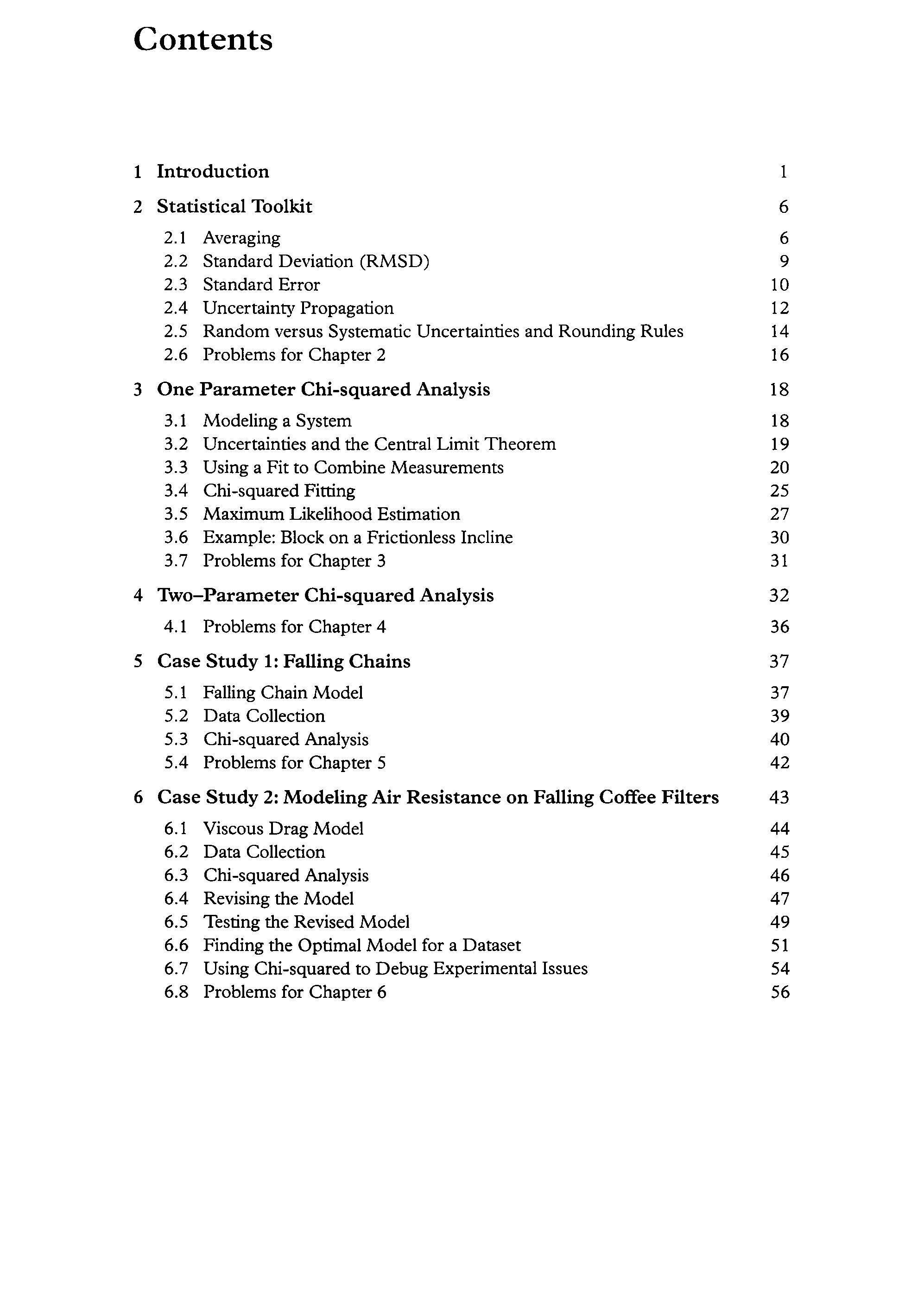
1 Introduction
2 Statistical Toolkit
2.1 Averaging
2.2 Standard Deviation (RMSD)
2.3 Standard Error
2.4 Uncertainty Propagation
2.5 Random versus Systematic Uncertainties and Rounding Rules
2.6 Problems for Chapter 2
3 One Parameter Chi-squared Analysis
3.1 Modeling a System
3.2 Uncertainties and the Central Limit Theorem
3.3 Using a Fit to Combine Measurements
3.4 Chi-squared Fitting
3.5 Maximum Likelihood Estimation
3.6 Example: Block on a Frictionless Incline
3.7 Problems for Chapter 3
4 Two-Parameter Chi-squared Analysis
4.1 Problems for Chapter 4
5 Case Study 1: Falling Chains
5.1 Falling Chain Model
5.2 Data Collection
5.3 Chi-squared Analysis
5.4 Problems for Chapter 5
6 Case Study 2: Modeling Air Resistance on Falling Coffee Filters
6.1 Viscous Drag Model
6.2 Data Collection
6.3 Chi-squared Analysis
6.4 Revising the Model
6.5 Testing the Revised Model
6.6 Finding the Optimal Modelfor a Dataset
6.7 Using Chi-squared to Debug Experimental Issues
6.8 Problems for Chapter 6
Introduction
Say you discover a phenomenonthat you thinkis interesting or important or by some miracle both. You want to understand and hopefully use your discovery to help the world, so using your knowledge of science and mathematics you derive a simple mathematical model that explains how the phenomenon works. You conclude that there is somevariable y that depends on some other variable x that you can control. The simplest version of a model is that they are the same, that y = x. You probablyaren t this lucky, and other parameters that you don t control, like A and B, show up in your model. A simple example ofthis is the linear model y = Ax + B. You don t control A or B, but if you had some way of estimating their values, you could predict ay for any x. Ofcourse,in real life, your model may have morevariables or parameters, and you might give them different names, but for now let s use the example ofy = Ax + B.
What we want is a way to estimate the parameter values (A and B) in your model. In addition to that, we d like to know the uncertainties of those estimates. It takes a little extra work to calculate the uncertainties, but you need them to give your prediction teeth imaginehowdifficult itwould be to meaningfully interpret a prediction with 100% uncertainties! But even that isn t enough. We could make parameter estimates for any model, but that alone wouldn t tell us whether we had a good model. We d also like to know that the model in which the parameters appearcan pass some kind ofexperimental goodnessoffit test. A go/no go or accept/reject criterion would be nice. Ofcourse,there s no test you can perform thatwill provide a believable binary result of congratulations, you gotit right! or wrong model, but keep trying. We can hopefor relative statements of better or worse, some sort of continuous (not binary) metric that allows comparison between alternatives, but not a statement ofabsolute truth.
Summarizing so far, we ve specified four requirements for a method ofanalyzing data collected on a system for which a modelis available:
Since the general problem we presented (parameter estimation and model testing) is a universal one andsince the specific requirements we came up with to solve the problem arefairly straightforward, you might expect there to be a generally accepted solution to the problem that is used by everyone. The good newsis that there is a generally accepted methodto solve the problem. The bad newsis thatit is not used by everyone andthe people whodouseit rarely explain howto useit (intelligibly, anyway).
That s why wewrote this book.
This generally accepted solution to the system parameter estimation and model testing problem is used by physicists to analyze results of some of the most precise and significant experiments of our time, including those that led to the discoveries of the Higgs boson and gravitational waves. We teach the method in our freshman/sophomore introductory physics laboratory course at Harvard University, called Principles of Scientific Inquiry. Using the software available at this book s website to perform the necessary calculations (the method is easy to understand but computation intensive), the method could be taught in high schools, used by more than the few researchers who useit now, and used in many morefields.
The method is called chi-squared analysis (x? analysis, pronounced kai-squared ) and will be derived in Chapter 3 using the maximum likelihood method.If in high schoolor college you tested a hypothesis by checking whether the differencebetweenexpected and observedfrequencies wassignificantin afruit fly or bean experiment, you likely performed the count data form of chi-squared analysis introduced bystatistician Karl Pearson. Karl Pearson s chi-squared test was included in an American Association for the Advancementof Sciencelist of the top twenty discoveries of the twentieth century.! The version of chi-squared analysis that you will learn from this book works with continuous data, the type of the data you get from reading a meter, and provides best fit model parameter values and model testing. Parameter estimation and modeltesting,all from one consistent, easy to apply method!
Butfirst, let s start with a practical example, looking at real data drawn from an introductory physics lab experimentrelating the length and period ofa pendulum. The period of a simple pendulum depends onits length and is often given by T=2nJE. This pendulum modelisn t linear, but it can be cast in the linear form y = Ax as follows: L= aT , where X =T?, Y=L, and A= gt: However, something seems to be wrong here. In this experiment we change the length (L) and observe the period (T), yet L in the model is the dependentvariable y! There s a reason for this. One of the simplifications we will be using throughout most of this book is the assumption that all uncertainties are associatedwith measurementsofthe dependentvariable y. You might think that measurements of pendulum length should have even less uncertainty
1 Hacking,I. (1984). Science 84, 69-70.
than pendulum period, but we assure you that from experience teaching many, many, physics lab sections, it doesn t! The accuracy of photogate sensors or video analysis, coupled with the large number of period measurements that can be averaged, makes the uncertainty in period data fairly small, while meter stick measurements, especially when long pendulums(greater than a meter) are involved, often exhibit surprisingly large uncertainties.
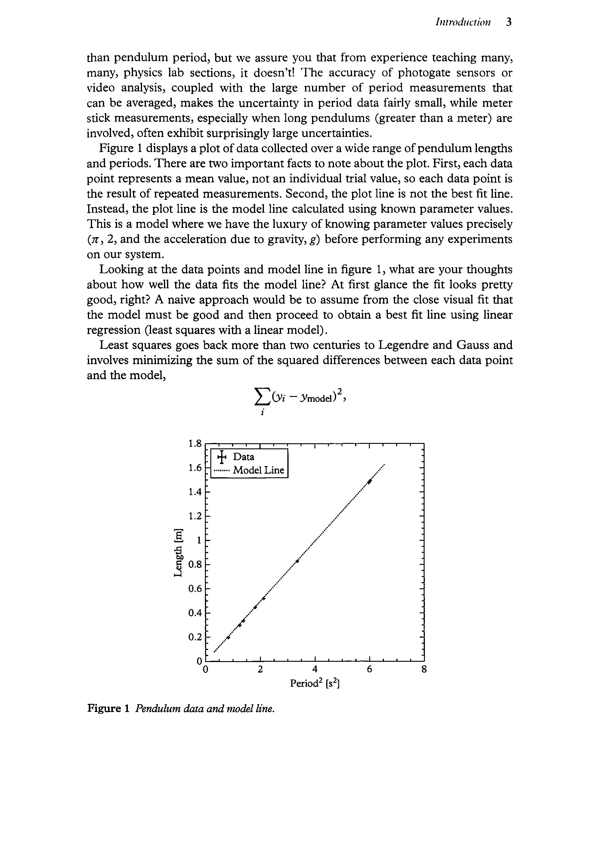
Figure 1 displays a plot ofdata collected over a wide range ofpendulum lengths and periods. There are two importantfacts to note aboutthe plot. First, each data point represents a mean value, not an individualtrial value, so each data pointis the result of repeated measurements. Second,the plot line is not the best fit line. Instead, the plot line is the model line calculated using known parameter values. This is a model where we havethe luxury ofknowing parametervaluesprecisely (2, 2, and the acceleration due to gravity, g) before performing any experiments on our system.
Looking at the data points and modelline in figure 1, what are your thoughts about how well the data fits the model line? At first glance the fit looks pretty good, right? A naive approach would be to assume from theclose visual fit that the model must be good and then proceed to obtain a best fit line using linear regression (least squares with a linear model).
Least squares goes back more than two centuries to Legendre and Gauss and involves minimizing the sum of the squared differences between each data point and the model,
Yor _- Ymodel) s i
Figure 1 Pendulum data and model line.
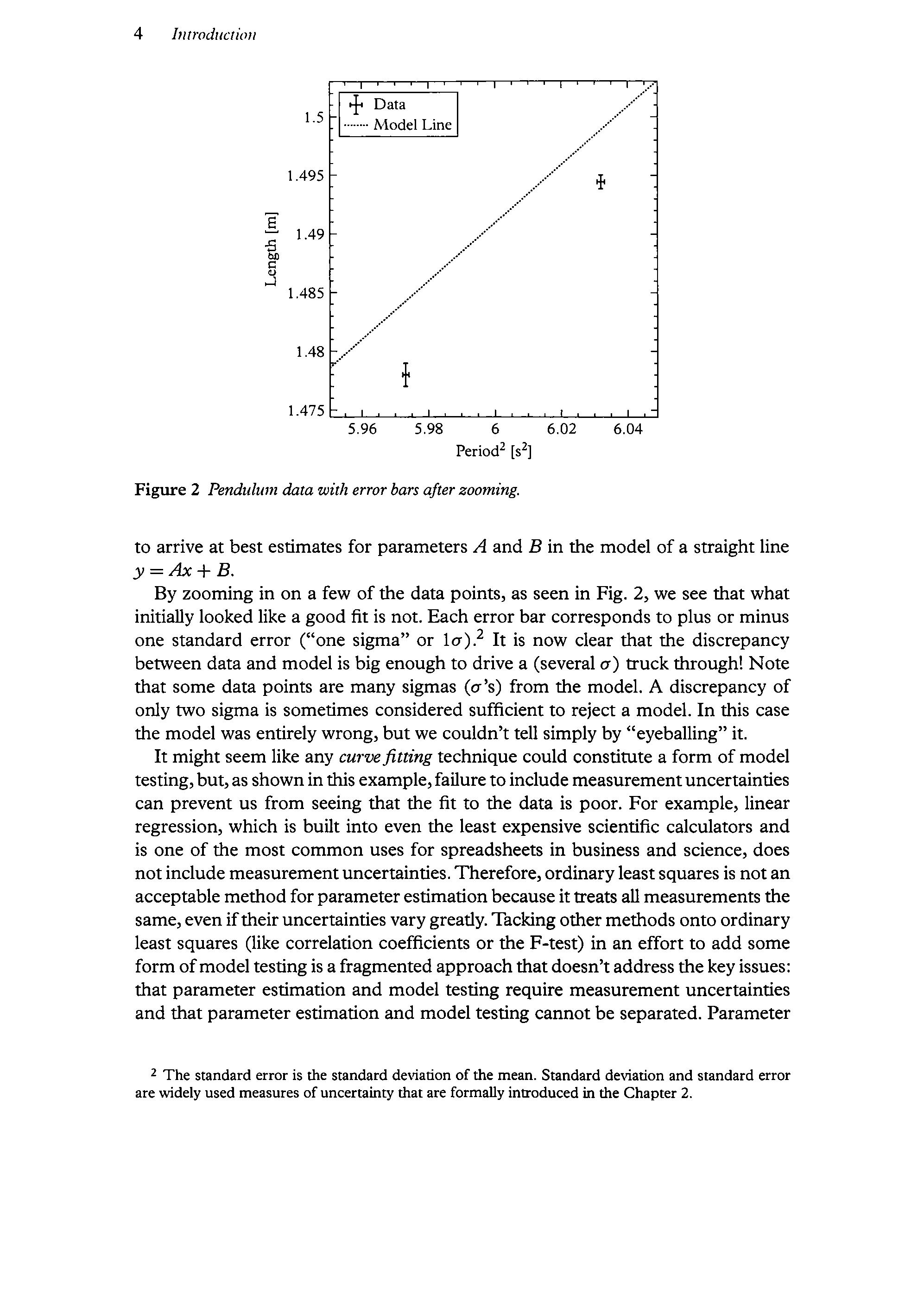
Figure 2 Pendulum data with error bars afterzooming.
to arrive at best estimates for parameters A and B in the model ofa straight line y= Axt B.
By zooming in on a few ofthe data points, as seen in Fig. 2, we see that what initially looked like a good fit is not. Each error bar correspondsto plus or minus one standard error ( one sigma or 1o).? It is now clear that the discrepancy between data and model is big enoughto drive a (several o) truck through! Note that some data points are many sigmas (o s) from the model. A discrepancy of only two sigma is sometimes considered sufficient to reject a model. In this case the model was entirely wrong, but we couldn t tell simply by eyeballing it. It might seem like any curvefitting technique could constitute a form of model testing,but,as shownin this example,failureto include measurementuncertainties can prevent us from seeing that the fit to the data is poor. For example, linear regression, which is built into even the least expensive scientific calculators and is one of the most commonuses for spreadsheets in business and science, does not include measurementuncertainties. Therefore, ordinaryleastsquares is notan acceptable methodforparameterestimationbecauseittreats all measurements the same,even iftheiruncertainties vary greatly. Tacking other methods onto ordinary least squares (like correlation coefficients or the F-test) in an effort to add some form ofmodel testing is a fragmented approachthatdoesn taddressthe keyissues: that parameter estimation and model testing require measurement uncertainties and that parameter estimation and model testing cannot be separated. Parameter
2 The standard erroris the standard deviation of the mean. Standard deviation and standard error are widely used measures ofuncertainty that are formally introducedin the Chapter2.
estimation and modeltesting is a chicken or egg problem: how can we know if a modelis good withoutfirst estimating its parameters, yet how can weestimate meaningful model parameters without knowingifthe model is good?
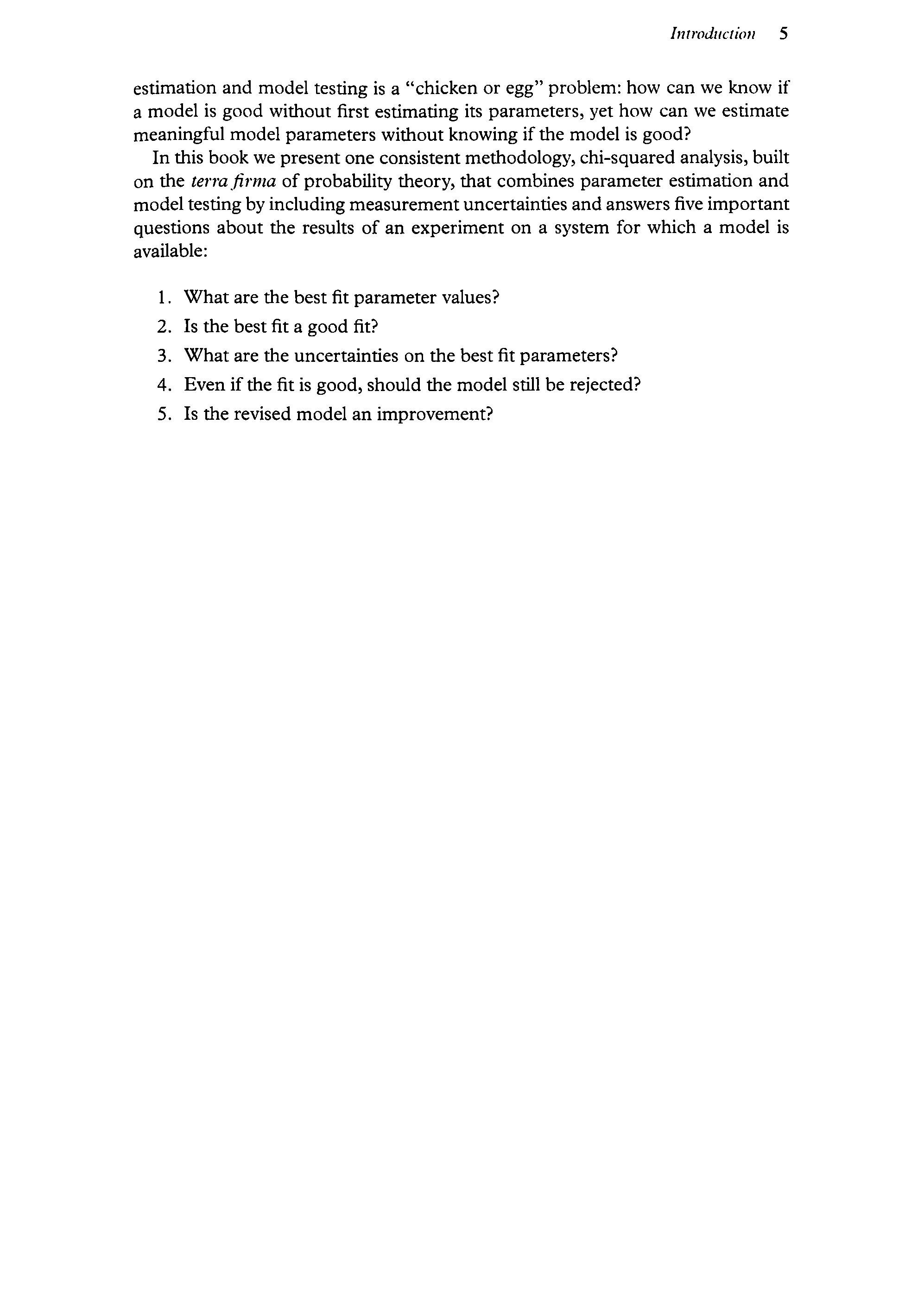
In this book we present one consistent methodology, chi-squared analysis, built on the terrafirma of probability theory, that combines parameter estimation and modeltesting by including measurement uncertainties and answersfive important questions about the results of an experiment on a system for which a modelis available:
Whatare the best fit parameter values?
Is the bestfit a goodfit?
Whatare the uncertainties on the bestfit parameters?
Evenifthe fit is good, should the modelstill be rejected?
Is the revised model an improvement?
2 Statistical Toolkit
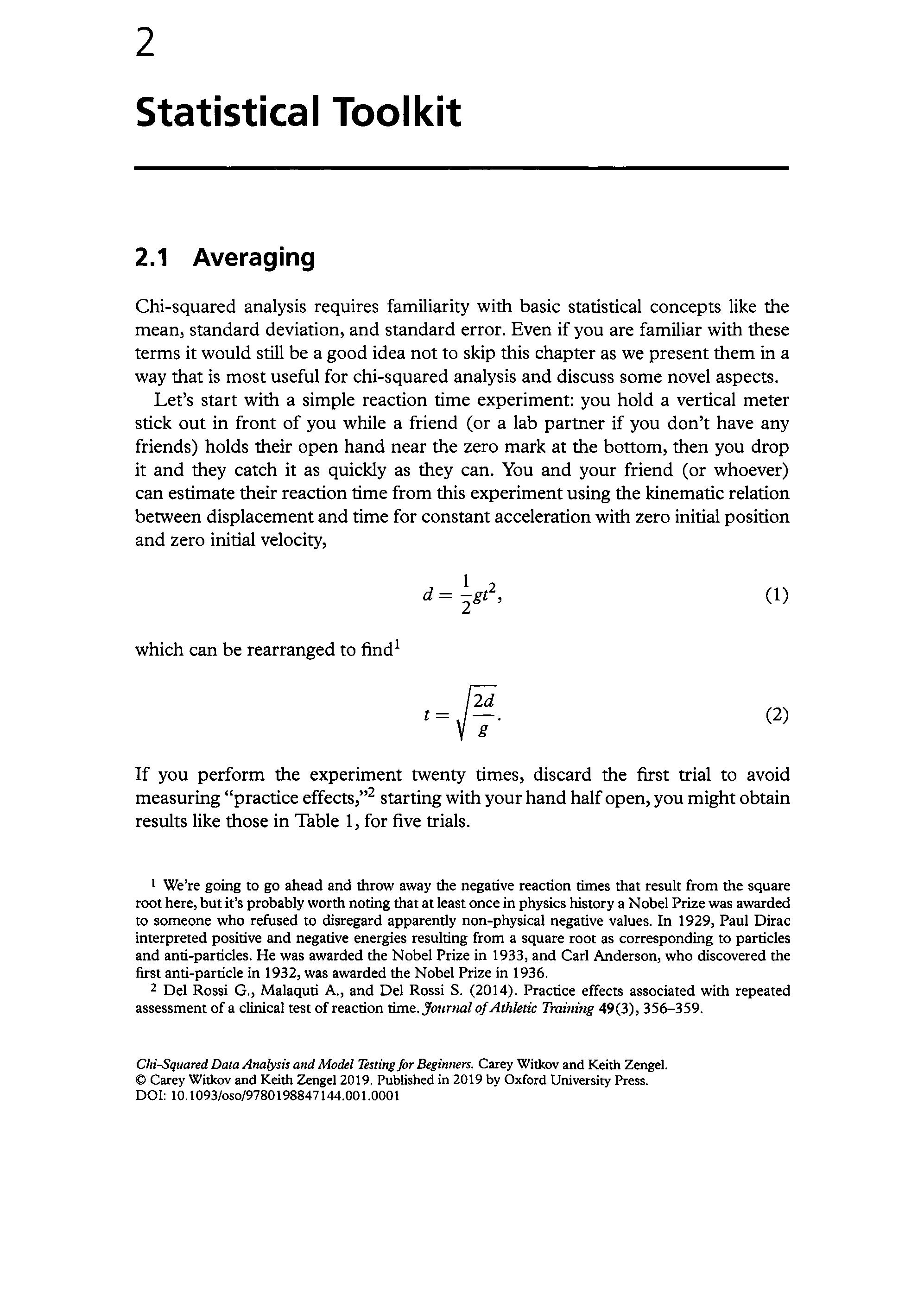
2.1 Averaging
Chi-squared analysis requires familiarity with basic statistical concepts like the mean, standard deviation, and standard error. Even if you are familiar with these termsit would still be a good idea not to skip this chapter as we present them in a way that is most useful for chi-squared analysis and discuss some novelaspects. Let s start with a simple reaction time experiment: you hold a vertical meter stick out in front of you while a friend (or a lab partner if you don t have any friends) holds their open hand near the zero mark at the bottom, then you drop it and they catch it as quickly as they can. You and your friend (or whoever) can estimate their reaction time from this experiment using the kinematic relation between displacementand time for constant acceleration with zeroinitial position and zeroinitial velocity,
If you perform the experiment twenty times, discard the first trial to avoid measuring practice effects, * startingwith yourhandhalfopen,you mightobtain results like those in Table 1, forfivetrials.
! We re going to go ahead and throw awaythe negative reaction times that result from the square roothere,butit s probably worth noting that at least once in physics history a Nobel Prize was awarded to someone whorefused to disregard apparently non-physical negative values. In 1929, Paul Dirac interpreted positive and negative energies resulting from a square root as corresponding to particles and anti-particles. He was awarded the Nobel Prize in 1933, and Carl Anderson, who discovered the first anti-particle in 1932, was awarded the NobelPrize in 1936.
2 Del Rossi G., Malaquti A., and Del Rossi S. (2014). Practice effects associated with repeated assessmentofa clinical test ofreaction time.JournalofAthletic Training 49(3), 356-359.
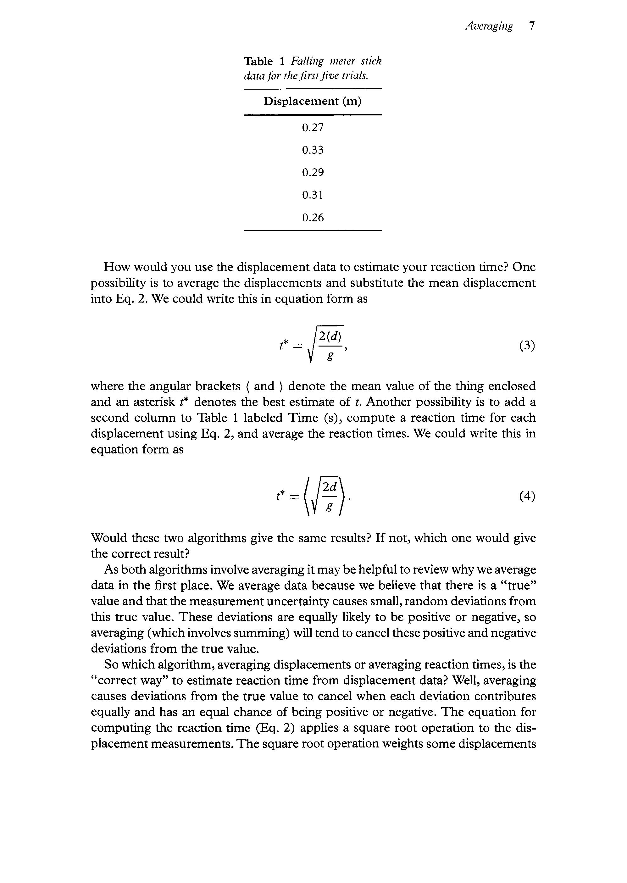
Table 1 Falling meter stick dataforthefirstfive trials. Displacement (m)
How would you use the displacement data to estimate your reaction time? One possibility is to average the displacements and substitute the mean displacement into Eq. 2. We could write this in equation form as
where the angular brackets ( and ) denote the mean value of the thing enclosed and an asterisk ¢* denotes the best estimate of t. Another possibility is to add a second column to Table 1 labeled Time (s), compute a reaction time for each displacement using Eq. 2, and average the reaction times. We could write this in equation form as
Would these two algorithms give the sameresults? If not, which one would give the correct result?
As both algorithmsinvolve averaging itmay be helpful to review whywe average data in the first place. We average data because webelieve that there is a true value and thatthe measurementuncertainty causes small,random deviations from this true value. These deviations are equally likely to be positive or negative, so averaging (which involves summing) will tend to cancel thesepositive and negative deviations from the true value.
So which algorithm, averaging displacements or averaging reaction times, is the correct way to estimate reaction time from displacement data? Well, averaging causes deviations from the true value to cancel when each deviation contributes equally and has an equal chanceof being positive or negative. The equation for computing the reaction time (Eq. 2) applies a square root operation to the displacement measurements. The square root operation weights some displacements
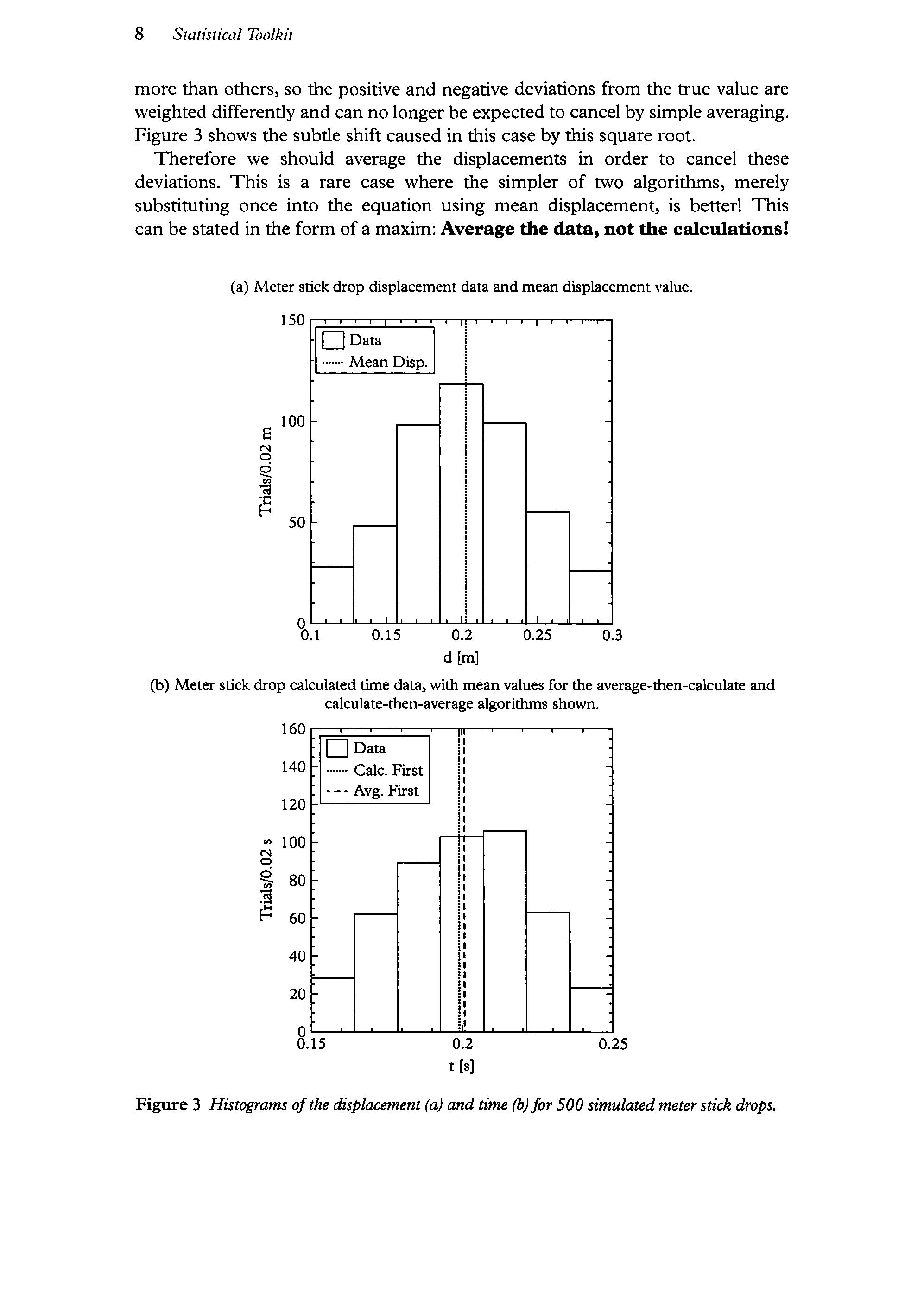
more than others, so the positive and negative deviations from the true value are weighted differently and can no longer be expected to cancel by simple averaging. Figure 3 showsthe subtle shift caused in this case by this square root.
Therefore we should average the displacements in order to cancel these deviations. This is a rare case where the simpler of two algorithms, merely substituting once into the equation using mean displacement, is better! This can bestated in the form ofa maxim: Averagethe data, not the calculations!
(a) Meter stick drop displacement data and mean displacementvalue. VSO ro or H {__] Data ot MeanDisp.
(b) Meterstick drop calculated time data, with mean values for the average-then-calculate and calculate-then-average algorithms shown.
Figure 3 Histograms ofthe displacement (a) and time (b)for 500 simulated meterstick drops.
2.2 Standard Deviation (RMSD)
Let s say you and yourfriend (or whoever) thoughtthis calculated reaction time was an important scientific result. You write a paper on your experiment and results and send it to The fournal of Kinesthetc Experiments (The JoKE), but it gets bounced back. You left something out. You forgot to include an estimate of uncertainty in your reaction time. The uncertainty in your reaction time depends on the spread (synonyms:dispersion, scatter, variation) in the data. How do you characterize the spread in data? Listing all ofyour data is usually difficult to read and impractical. Giving highs and lows is better than nothing (though not by much)as they disregardall ofthe other data and onlycharacterize outliers. Taking the deviation (difference) ofeach value from the mean seems useful but runs into the problem that the meandeviationis zero.
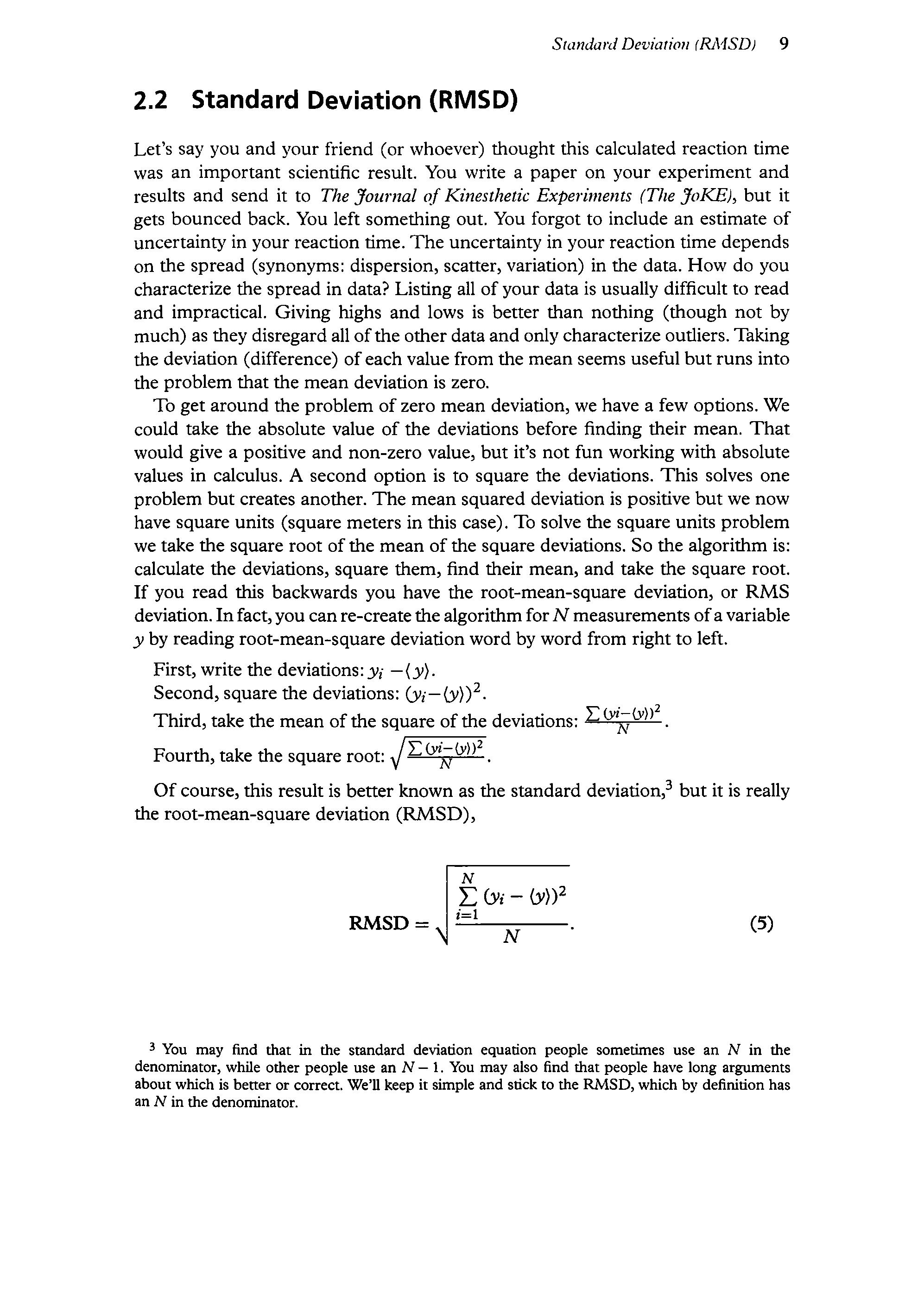
To get around the problem of zero mean deviation, we have a few options. We could take the absolute value of the deviations before finding their mean. That would give a positive and non-zero value, butit s not fun working with absolute values in calculus. A second option is to square the deviations. This solves one problem but creates another. The mean squared deviation is positive but we now have square units (square meters in this case). To solve the square units problem wetake the square root ofthe mean of the square deviations. So the algorithm is: calculate the deviations, square them, find their mean, and take the square root. If you read this backwards you have the root-mean-square deviation, or RMS deviation. Infact,you can re-createthe algorithm forN measurementsofa variable y by reading root-mean-square deviation word by word from righttoleft.
First, write the deviations:y; (y).
Second, square the deviations: (y; (y))?. . 2
Third, take the mean of the square of the deviations: LOE
Fourth, take the square root: \/ Lor|
Ofcourse, this result is better known asthe standard deviation, butit is really the root-mean-square deviation (RMSD),
3 You may find that in the standard deviation equation people sometimes use an N in the denominator, while other people use an N 1. You mayalso find that people have long arguments about which is better or correct. We'll keep it simple and stick to the RMSD,which by definition has an N in the denominator.
2.3. Standard Error
You resubmit yourresults to TheJoKE, this tme presenting your mean reaction displacementplus or minusits standard deviation,but yoursubmission is bounced back again. The editor explains that the standard deviation does not measure uncertainty in your mean reaction displacement. Then what does standard deviation measure?
The standard deviation measures the spread ofyour entire set ofmeasurements. In this experiment, the standard deviation of the displacements represents the uncertainty ofeach individual displacement measurement.
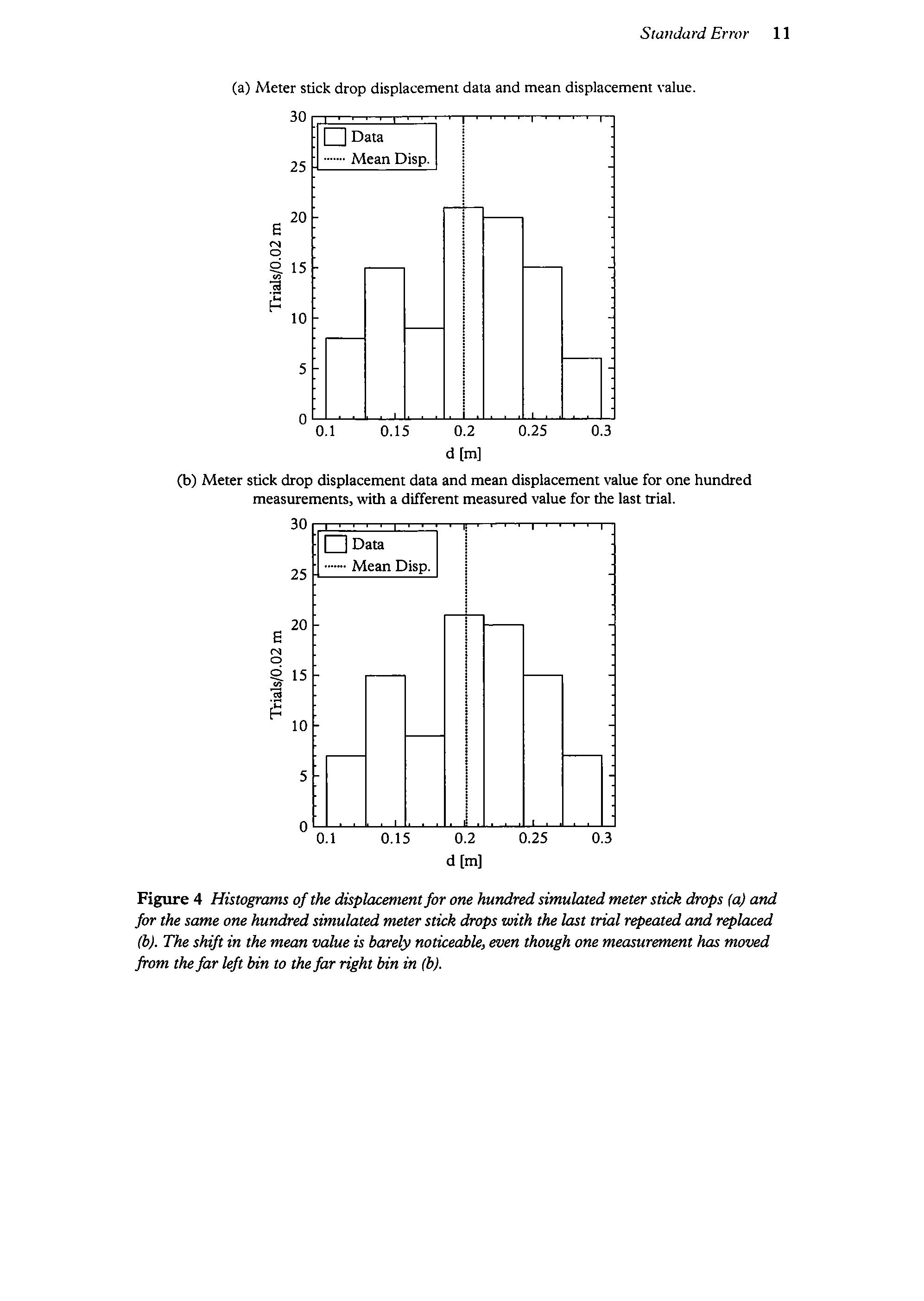
But the uncertainty of an individual measurementis not the uncertainty ofthe mean ofthe measurements, Consider the (mercifully) hypothetical case oftaking a hundred measurements ofyourreaction time. Ifyou repeated and replaced one ofyour measurements, you wouldn t be surprisedifit was one standard deviation from the mean value of your original 100 measurements. But unless you were usinga verylong stickandsomethingwentterribly,medicallywrong,you wouldn t expect the mean value of your new set of a hundred measurements to be very different from the mean value ofyour original hundred measurements. See figure 4 for an example of data from one hundred measurements, with and without the last trial repeated and replaced.
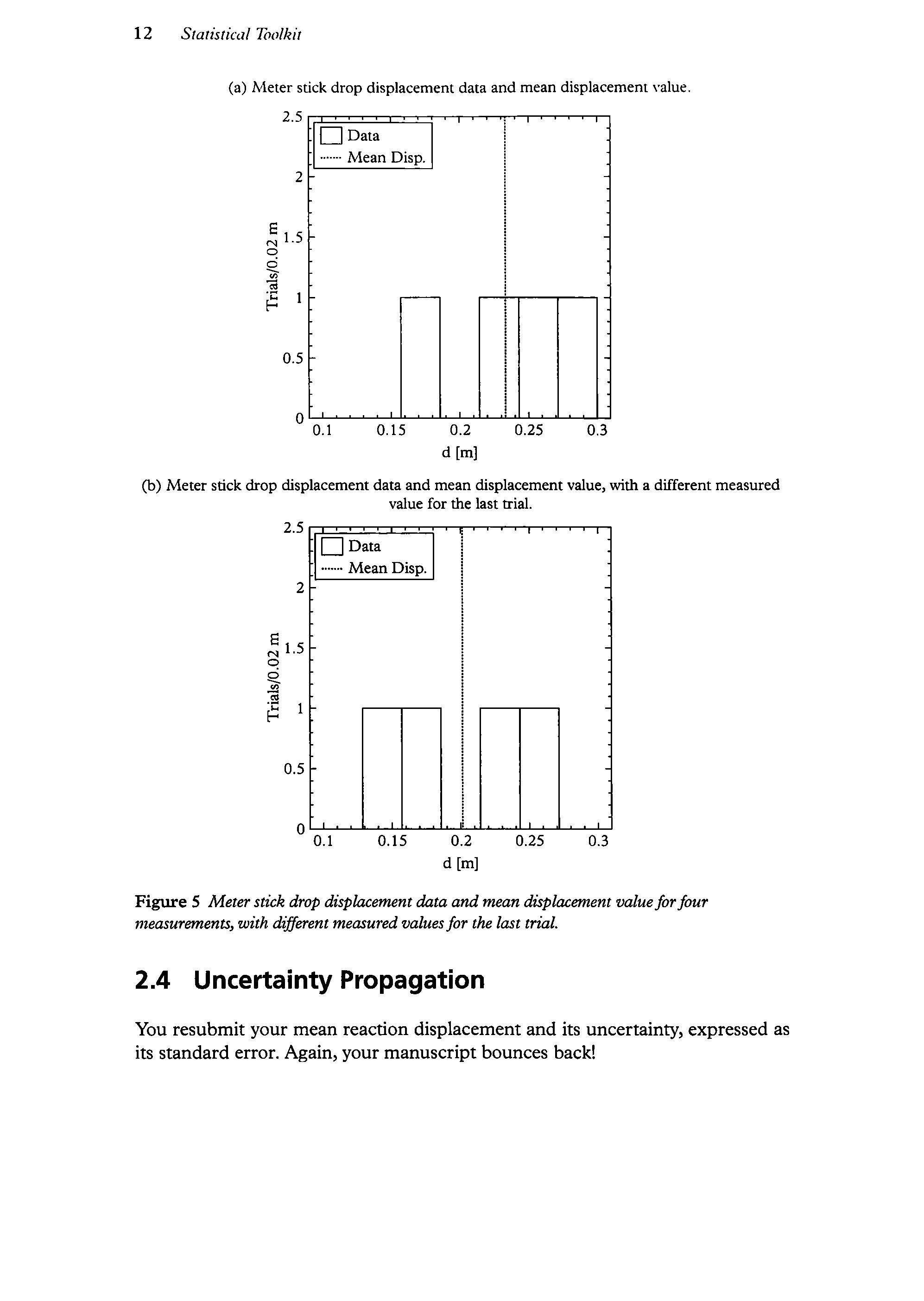
Now consider the hypothetical case oftaking only four measurements, finding the mean and standard deviation, and then repeating and replacing one ofthose measurements. See figure 5 for an example ofdata from four measurements,with and withoutthe last trial repeated and replaced. You would still find it perfectly natural if the new measurement were one standard deviation from the mean of your original four measurements, but you also wouldn t be so surprised or find much reason for concern for your health if your new mean value shifted by a considerable amount. In other words, the uncertainty ofyour next measurement (the standard deviation) won t changeall that much as you take more data, but the uncertainty on the mean of your data should get smaller as you take more data. This is the same logic we used previously to explain why we averaged the displacementdata: every measurement includes some fluctuation around the true value, which cancels out when we take the average. We don t expect these experimental uncertainties to be magically resolved before the nexttrial,but as we take more data, the mean valueis less susceptible to being significantly shifted by the fluctuation in any one particular measurement.
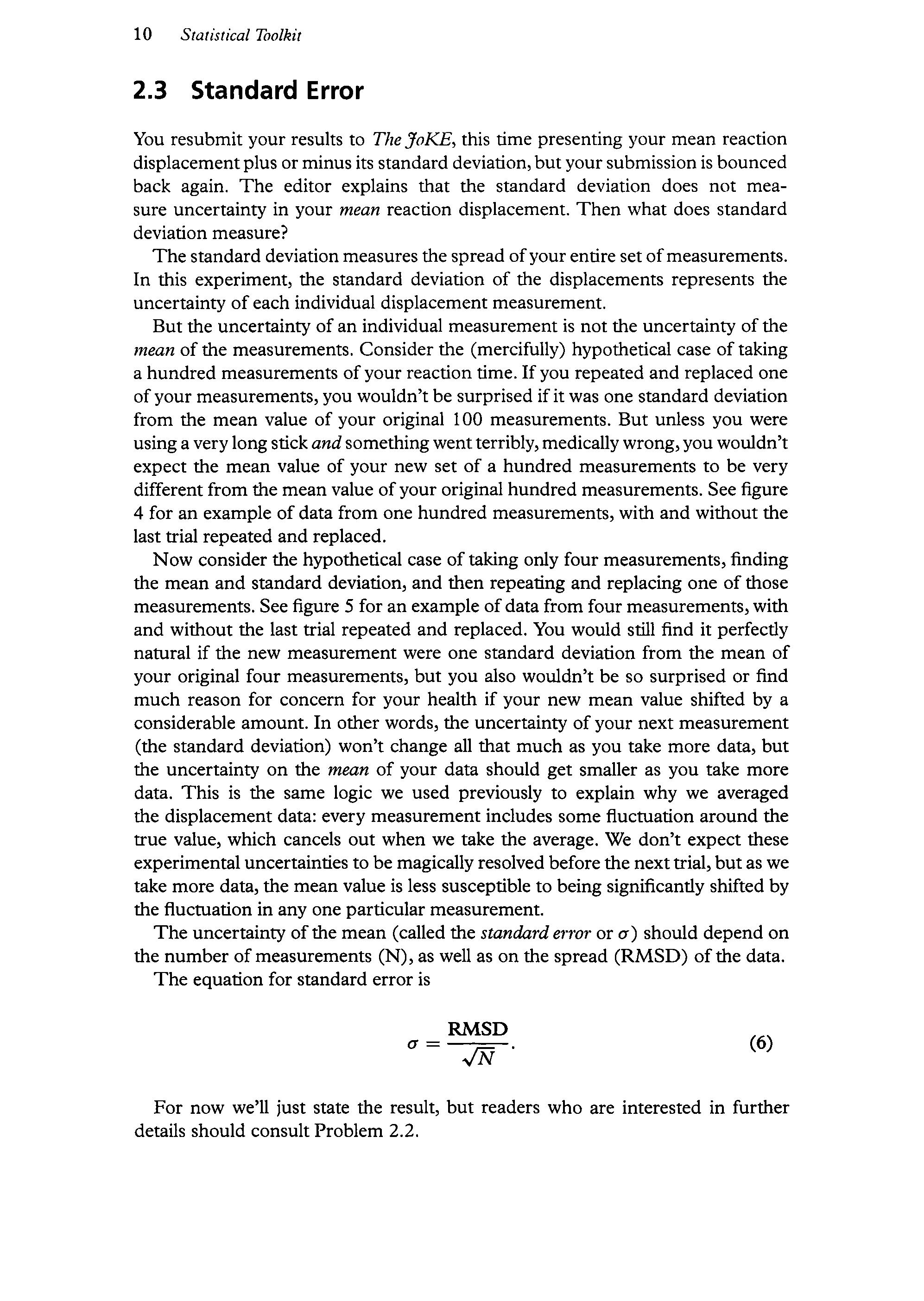
The uncertainty ofthe mean (called the standarderror or o) should depend on the number ofmeasurements (N), as well as on the spread (RMSD)ofthe data.
The equation for standarderroris
0 = Ty (6)
For now we'll just state the result, but readers whoare interested in further details should consult Problem 2.2.
(a) Meter stick drop displacement data and mean displacementvalue.
oe +] L_] Data
(b) Meterstick drop displacement data and mean displacementvalue for one hundred measurements, with a different measured value forthelasttrial.
Cc [_] Data
Figure 4 Histograms ofthe displacementfor one hundredsimulatedmeterstick drops (a) and jor the same one hundredsimulated meterstick drops with the last trial repeated and replaced (b). The shift in the mean value is barely noticeable, even though one measurement has moved from thefarleft bin to thefar right bin in (b).
(a) Meter stick drop displacement data and mean displacementvalue.
(b) Meterstick drop displacement data and mean displacementvalue, with a different measured value for the lasttrial.
Figure 5 Meterstick drop displacement data and mean displacement valueforfour measurements, with different measured valuesfor the lasttrial.
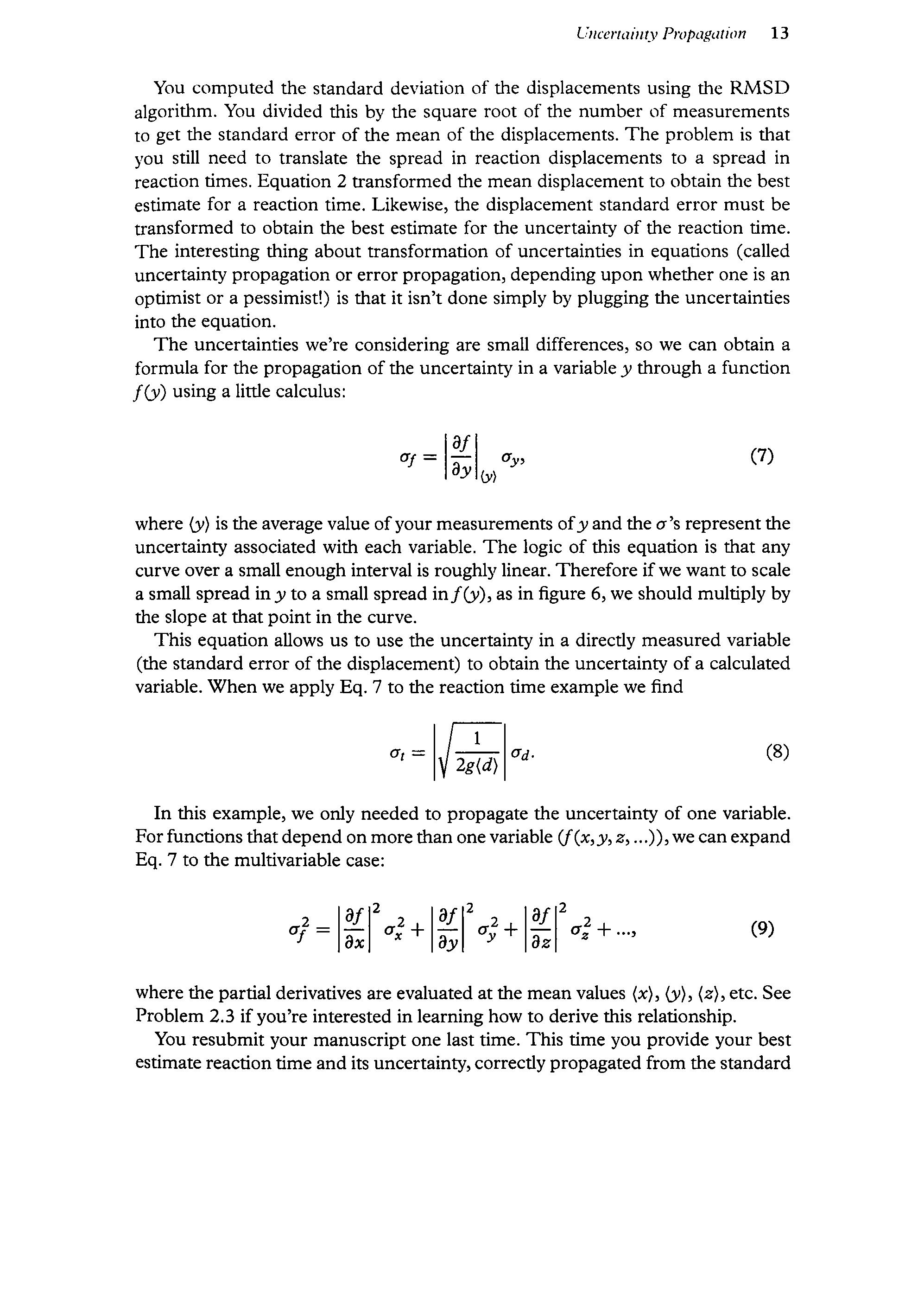
2.4 Uncertainty Propagation
You resubmit your mean reaction displacement and its uncertainty, expressed as its standard error. Again, your manuscript bounces back!
You computed the standard deviation of the displacements using the RMSD algorithm. You divided this by the square root of the number of measurements to get the standard error of the mean ofthe displacements. The problem is that you still need to translate the spread in reaction displacements to a spread in reaction times, Equation 2 transformed the mean displacementto obtain the best estimate for a reaction time. Likewise, the displacement standard error must be transformed to obtain the best estimate for the uncertainty of the reaction time. The interesting thing about transformation of uncertainties in equations (called uncertainty propagation or error propagation, depending upon whetheroneis an optimist or a pessimist!) is that it isn t done simply by plugging the uncertainties into the equation.
The uncertainties we re considering are small differences, so we can obtain a formula for the propagation of the uncertainty in a variable y through a function f(y) using a little calculus:
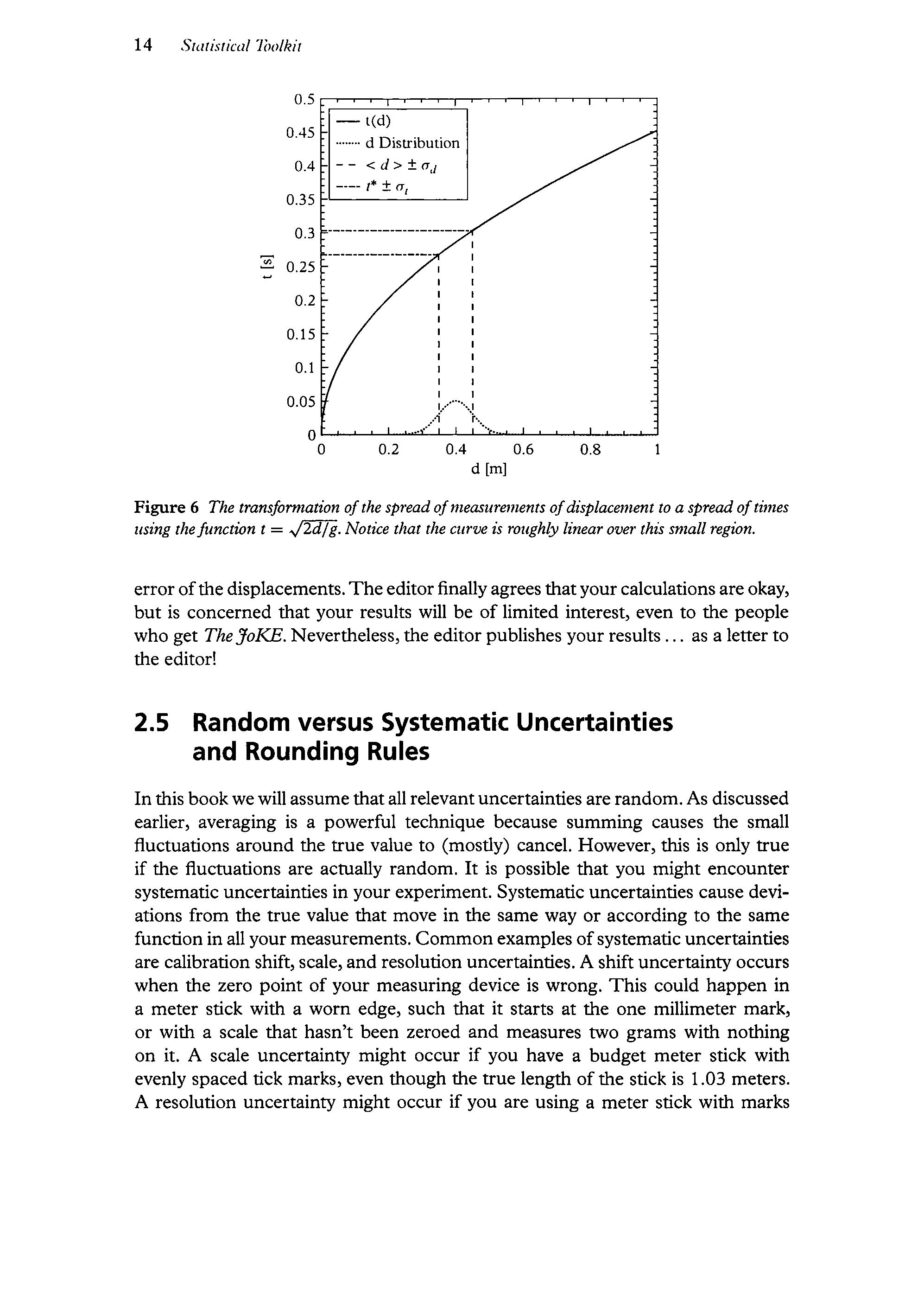
where(y) is the average value ofyour measurementsofy and the o s represent the uncertainty associated with each variable. The logic of this equation is that any curve over a small enoughinterval is roughlylinear. Therefore ifwe want to scale a small spread iny to a small spread inf(y),as in figure 6, we should multiply by the slope at that point in the curve.
This equation allows us to use the uncertainty in a directly measured variable (the standard error of the displacement) to obtain the uncertainty ofa calculated variable. When we apply Eq. 7 to the reaction time example wefind
(8)
In this example, we only needed to propagate the uncertainty of one variable. Forfunctions thatdepend on more than onevariable (f(x,,2,...)),we can expand Eq. 7 to the multivariable case:
wherethe partial derivatives are evaluated at the mean values (x),(y), (2), etc. See Problem 2.3 ifyou re interested in learning how to derive this relationship.
You resubmit your manuscript onelast time. This time you provide your best estimate reaction time andits uncertainty, correctly propagated from the standard
Figure 6 The transformation ofthe spreadofmeasurements ofdisplacementto a spread oftimes using thefunction t = ./2d/g. Notice that the curve is roughly linear over this small region.
errorofthe displacements.Theeditorfinallyagrees thatyour calculations are okay, but is concerned that yourresults will be of limited interest, even to the people whoget TheJoKE. Nevertheless, the editor publishes yourresults... as a letter to the editor!
2.5 Random versus Systematic Uncertainties and Rounding Rules
Inthis bookwewill assumethatall relevantuncertainties are random.As discussed earlier, averaging is a powerful technique because summing causes the small fluctuations around the true value to (mostly) cancel. However, this is only true if the fluctuations are actually random.It is possible that you might encounter systematic uncertainties in your experiment. Systematic uncertainties cause deviations from the true value that move in the same way or according to the same functionin all your measurements. Commonexamples ofsystematic uncertainties are calibration shift, scale, and resolution uncertainties. A shift uncertainty occurs when the zero point of your measuring device is wrong. This could happen in a meter stick with a worn edge, such that it starts at the one millimeter mark, or with a scale that hasn t been zeroed and measures two grams with nothing on it. A scale uncertainty might occur if you have a budget meter stick with evenly spaced tick marks, even though the true length ofthe stick is 1.03 meters. A resolution uncertainty might occur if you are using a meter stick with marks
only at every centimeter, or a voltmeter that has tick marks at every volt, when measuring somethingthat varies at a smaller scale.
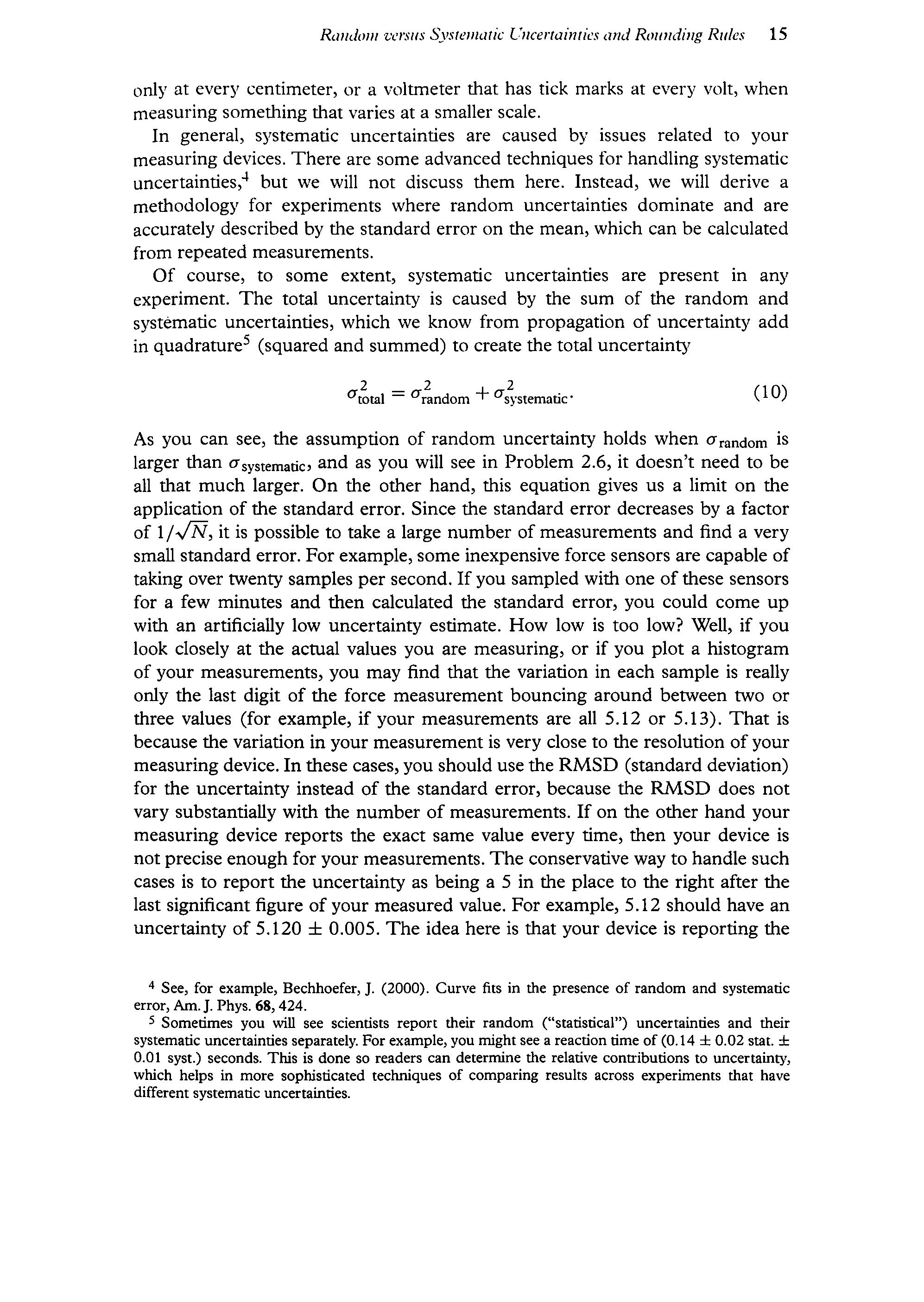
In general, systematic uncertainties are caused by issues related to your measuring devices. There are some advanced techniques for handling systematic uncertainties,* but we will not discuss them here. Instead, we will derive a methodology for experiments where random uncertainties dominate and are accurately described by the standard error on the mean, which can be calculated from repeated measurements.
Of course, to some extent, systematic uncertainties are present in any experiment. The total uncertainty is caused by the sum of the random and systematic uncertainties, which we know from propagation of uncertainty add in quadrature (squared and summed)to create the total uncertainty
Oral = Ovandom + OS.stematic* (10)
As you can see, the assumption of random uncertainty holds when oyandom is larger than O'systematic, and as you will see in Problem 2.6, it doesn t need to be all that much larger. On the other hand, this equation gives us a limit on the application of the standard error. Since the standard error decreases by a factor of 1//N,it is possible to take a large number of measurements and find a very small standard error. For example, some inexpensive force sensors are capable of taking over twenty samples per second. If you sampled with one ofthese sensors for a few minutes and then calculated the standard error, you could come up with an artificially low uncertainty estimate. How low is too low? Well, if you look closely at the actual values you are measuring, or if you plot a histogram of your measurements, you may find that the variation in each sampleis really only the last digit of the force measurement bouncing around between two or three values (for example, if your measurements are all 5.12 or 5.13). That is because the variation in your measurementis very close to the resolution ofyour measuring device. In these cases, you should use the RMSD (standard deviation) for the uncertainty instead of the standard error, because the RMSD does not vary substantially with the number of measurements. If on the other hand your measuring device reports the exact same value every time, then your device is not precise enough for your measurements. The conservative way to handle such cases is to report the uncertainty as being a 5 in the placeto the right after the last significant figure of your measured value. For example, 5.12 should have an uncertainty of 5.120 + 0.005. The idea here is that your device is reporting the
4 See, for example, Bechhoefer, J. (2000). Curve fits in the presence of random and systematic error, Am.J. Phys. 68, 424.
5 Sometimes you will see scientists report their random ( statistical ) uncertainties and their systematic uncertainties separately. For example, you might see a reaction time of (0.14 + 0.02 stat. 0.01 syst.) seconds. This is done so readers can determine the relative contributions to uncertainty, which helps in more sophisticated techniques of comparing results across experiments that have different systematic uncertainties.
most precise value it can, and that it would round up or down if the measurement were varying by more than this amount.
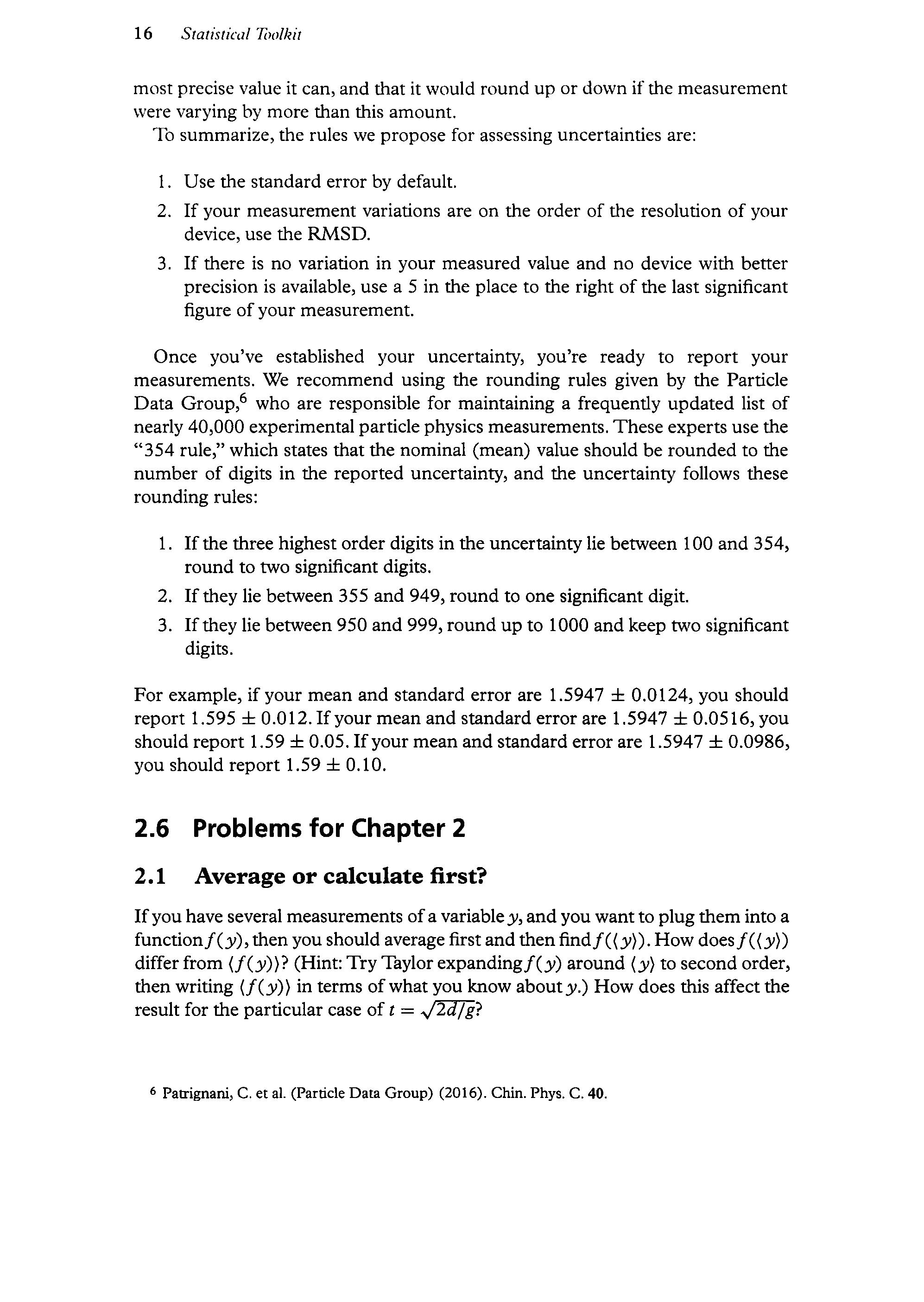
To summarize, the rules we propose for assessing uncertainties are:
1. Use the standard error by default.
2. If your measurementvariations are on the orderof the resolution of your device, use the RMSD.
3. If there is no variation in your measured value and no device with better precision is available, use a 5 in the place to the rightofthe last significant figure ofyour measurement.
Once you ve established your uncertainty, you re ready to report your measurements. We recommend using the rounding rules given bythe Particle Data Group,® whoare responsible for maintaining a frequently updatedlist of nearly 40,000 experimental particle physics measurements. These experts use the 354 rule, which states that the nominal (mean) value should be rounded to the number of digits in the reported uncertainty, and the uncertainty follows these rounding rules:
1. Ifthe three highest order digits in the uncertainty lie between 100 and 354, round to two significantdigits.
2. Ifthey lie between 355 and 949, roundto onesignificantdigit.
3. Ifthey lie between 950 and 999, round upto 1000 and keep twosignificant digits.
For example, if your mean and standard error are 1.5947 + 0.0124, you should report 1.595 + 0.012. Ifyour mean and standarderror are 1.5947 + 0.0516, you should report 1.59 + 0.05. Ifyour mean andstandarderror are 1.5947 + 0.0986, you should report 1.59 + 0.10.
2.6 Problems for Chapter 2
2.1 Average or calculatefirst?
Ifyou have several measurements ofa variabley, and you wantto plug them into a functionf(y),then you should averagefirst and thenfindf((y)). How doesf(()) differ from (f(y))? (Hint: Try Taylor expandingf(y) around (4) to second order, then writing (f(¥)) in terms ofwhat you know abouty.) How doesthis affect the result for the particular case of t = ./2d/g?
6 Patrignani, C.et al. (Particle Data Group) (2016). Chin. Phys. C. 40.
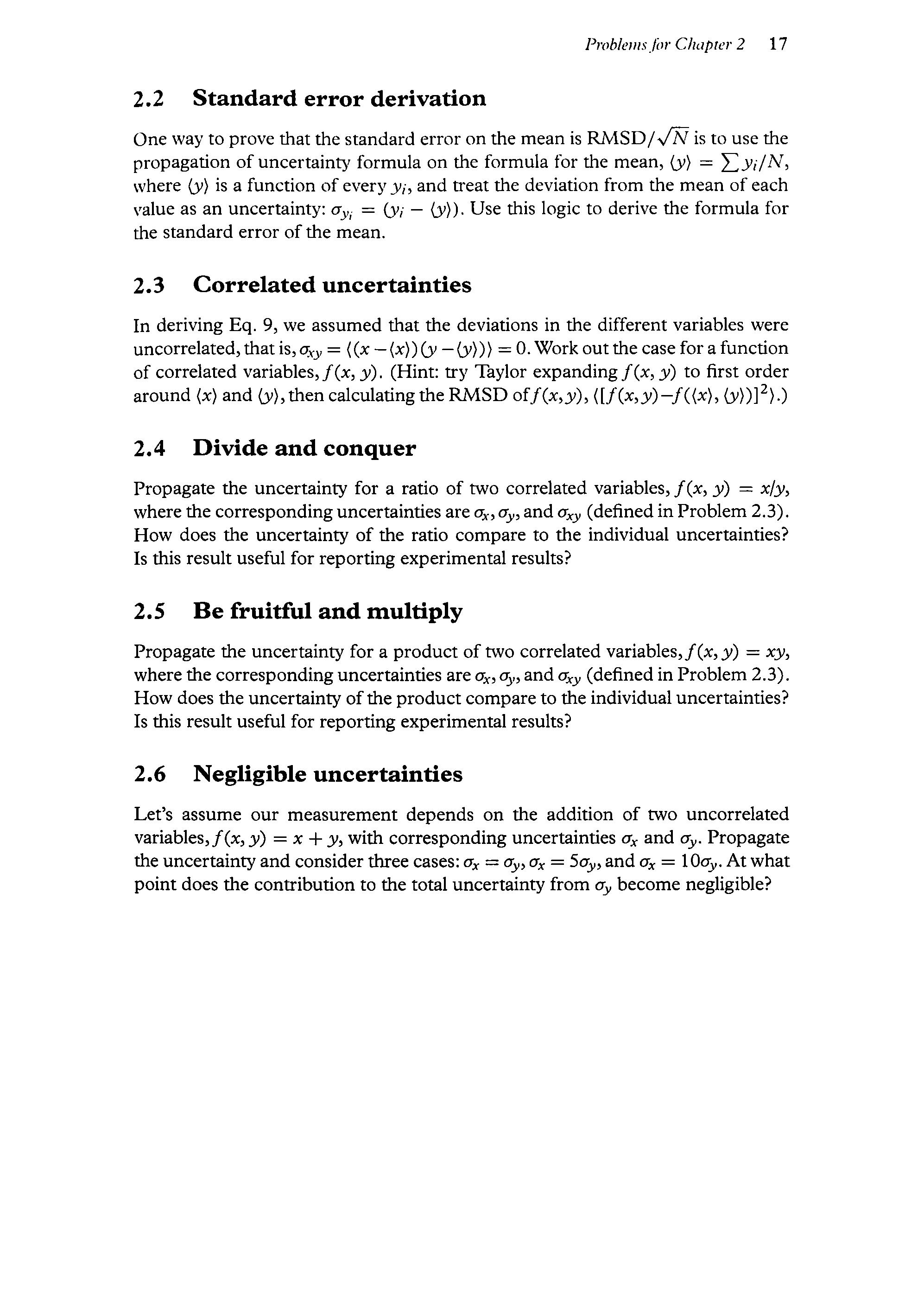
2.2. Standard error derivation
One wayto prove that the standard error on the mean is RMSD/JN is to use the propagation of uncertainty formula on the formula for the mean, (y) = 7yi/N, where (y) is a function of everyy;, and treat the deviation from the mean of each value as an uncertainty: oy, = (y; (y)). Use this logic to derive the formula for the standard error ofthe mean.
2.3 Correlated uncertainties
In deriving Eq. 9, we assumed that the deviations in the different variables were uncorrelated,thatis,ay = ((x (x))(vy (y))) = 0.Work outthe case for a function of correlated variables,f(x, y). (Hint: try Taylor expandingf(x, y) to first order around (x) and (y),then calculating the RMSDoff(x,y), (Lf(4.9) f(x), (v))]*).)
2.4 Divide and conquer
Propagate the uncertainty for a ratio of two correlated variables, f(x, vy) = x/v, where the correspondinguncertainties are o,,0,, and oy (defined in Problem 2.3). How does the uncertainty of the ratio compare to the individual uncertainties? Is this result useful for reporting experimental results?
2.5 Befruitful and multiply
Propagate the uncertainty for a product of two correlated variables,f(x,v) = xy, where the corresponding uncertainties are o,,a, and o,, (defined in Problem 2.3). How does the uncertainty ofthe product compareto the individual uncertainties? Is this result useful for reporting experimental results?
2.6 Negligible uncertainties
Let s assume our measurement depends on the addition of two uncorrelated variables,f(x, y) = x + y, with corresponding uncertainties o, and o,. Propagate the uncertainty and considerthree cases: 0, = dy, oy = Soy, and ox = 10cy. Atwhat point does the contribution to the total uncertainty from o, become negligible?
One Parameter Chi-squared Analysis
3.1 Modeling a System
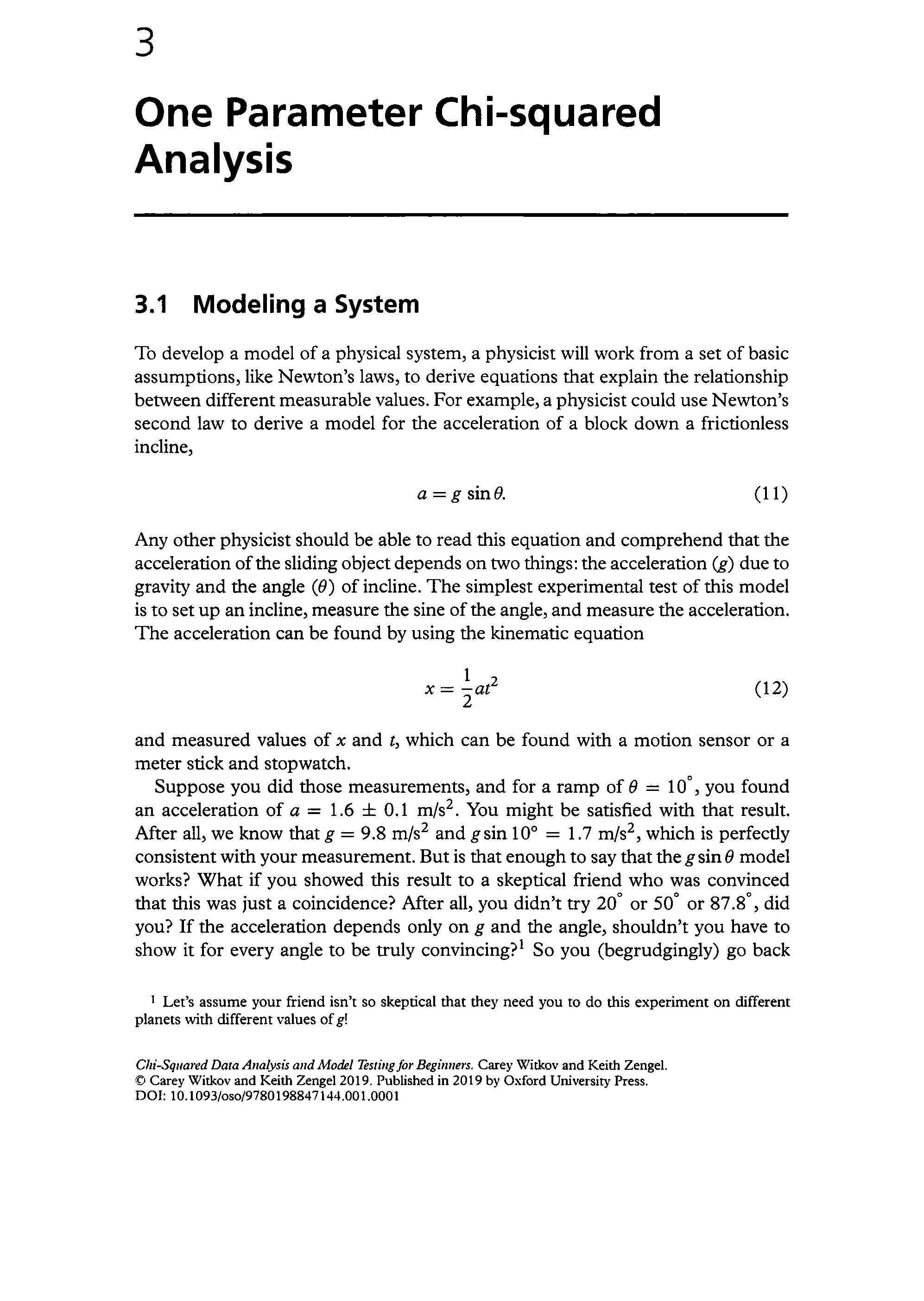
To develop a model ofa physical system, a physicist will work from a set of basic assumptions,like Newton s laws, to derive equations that explain the relationship between different measurable values. For example, a physicist could use Newton s second law to derive a model for the acceleration of a block down frictionless incline,
sing.
Any other physicist should be able to read this equation and comprehendthat the acceleration ofthe sliding objectdepends on twothings:the acceleration (g) due to gravity and the angle (6) ofincline. The simplest experimental test ofthis model is to set up an incline, measure the sine ofthe angle, and measurethe acceleration. The acceleration can be found by using the kinematic equation
1 2 x= 5at (12)
and measured values of x and t, which can be found with a motion sensor or a meter stick and stopwatch.
Suppose you did those measurements, and for a ramp of 6 = 10°, you found an acceleration of a = 1.6 + 0.1 m/s . You might be satisfied with that result. After all, we know that g = 9.8 m/s* and gsin 10° = 1.7 m/s?, whichis perfectly consistentwith your measurement. Butis that enoughto say thatthegsin9 model works? Whatif you showed this result to a skeptical friend who was convinced that this was just a coincidence? After all, you didn t try 20° or 50° or 87.8, did you? If the acceleration depends only on g and the angle, shouldn t you have to show it for every angle to be truly convincing?! So you (begrudgingly) go back
1 Let s assume yourfriend isn t so skeptical that they need you to do this experiment on different planets with different values ofg!
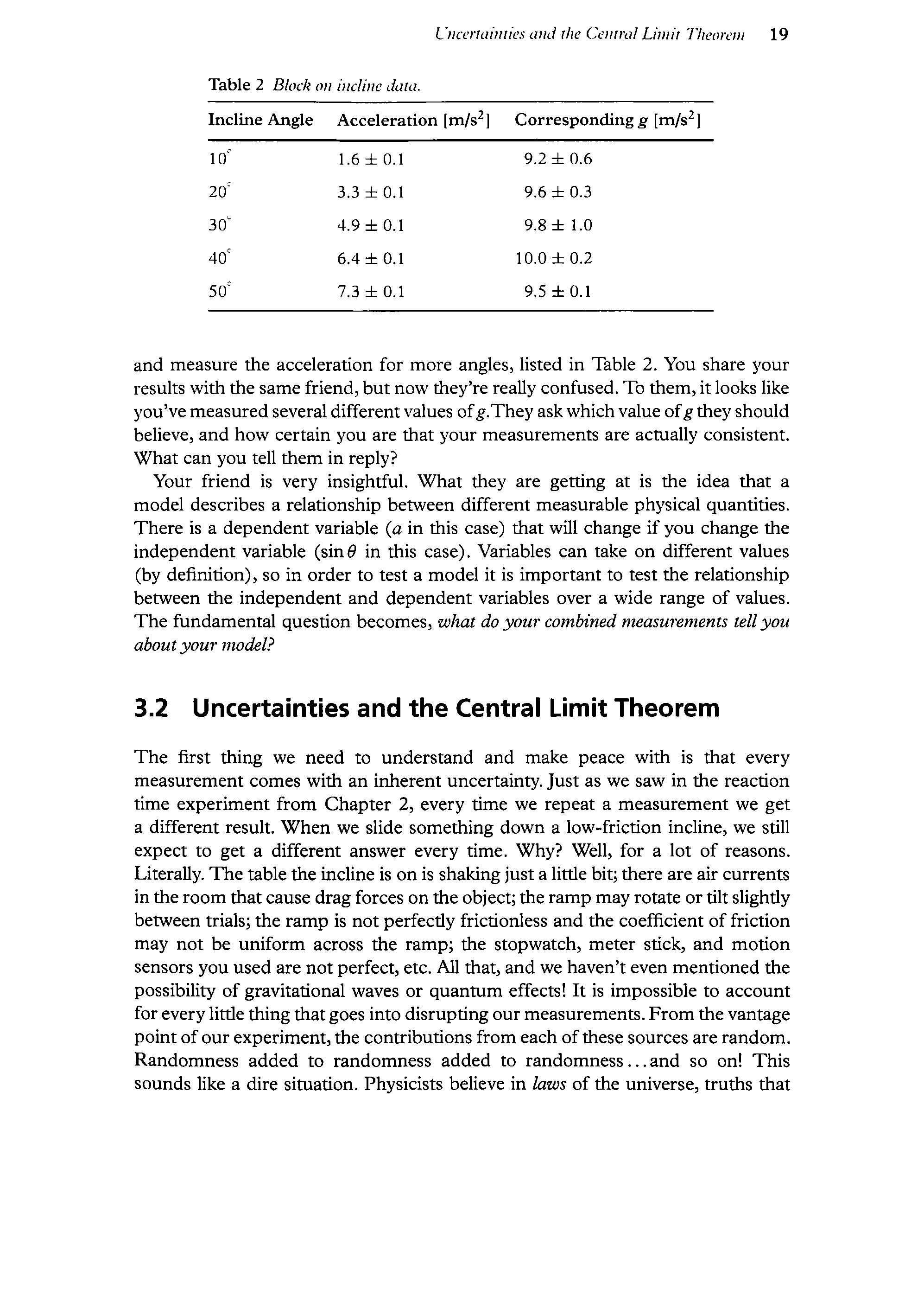
and measure the acceleration for more angles, listed in Table 2. You share your results with the same friend, but now they re really confused. To them,it lookslike you ve measuredseveral differentvalues ofg.They askwhichvalue ofgthey should believe, and how certain you are that your measurements are actually consistent. What can youtell them in reply?
Your friend is very insightful. What they are getting at is the idea that a model describes a relationship between different measurable physical quantities. There is a dependentvariable (a@ in this case) that will change if you change the independentvariable (sin@ in this case). Variables can take on different values (by definition), so in order to test a modelit is importantto test the relationship between the independent and dependentvariables over a wide range of values. The fundamental question becomes, what doyour combined measurements tellyou aboutyour model?
3.2 Uncertainties and the Central Limit Theorem
The first thing we need to understand and make peace with is that every measurement comes with an inherent uncertainty. Just as we saw in the reaction time experiment from Chapter 2, every time we repeat a measurement we get a different result. When we slide something down a low-friction incline, westill expect to get a different answer every time. Why? Well, for a lot of reasons. Literally. The table the incline is on is shakingjusta little bit; there are air currents in the room that cause drag forces on the object; the ramp mayrotateortilt slightly betweentrials; the rampis not perfectly frictionless and the coefficientoffriction may not be uniform across the ramp; the stopwatch, meter stick, and motion sensors you used are notperfect, etc. All that, and we haven t even mentioned the possibility of gravitational waves or quantum effects! It is impossible to account foreverylittle thing thatgoes into disrupting our measurements. From the vantage point ofour experiment, the contributions from each ofthese sources are random. Randomness added to randomness added to randomness...and so on! This soundslike a dire situation. Physicists believe in Jaws of the universe, truths that
are enforced and enacted everywhere and always. Yetthey never measure the same thing twice. Never. The randomness seems insurmountable, incompatible with any argumentfor the laws that physicists describe.
Exceptit s not.
What saves physicists from this nihilism is the Central Limit Theorem. The Central Limit Theorem is one of the most perplexing and beautiful results in all of mathematics.It tells us that when random variables are added, randomnessis not compounded,butrather reduced. An order emerges.
Formally, the Central Limit Theorem says that the distribution of a sum of random variables is well approximated by a Gaussian distribution (bell curve). The random variables being summed could have come from anydistribution or set of distributions (uniform, exponential, triangular, etc.). The particular set of underlying distributions being summed doesn t matter because the Central Limit Theorem says youstill get a Gaussian.
One benefit of the Central Limit Theorem is that experimenters measuring a deterministic process that is influenced by many small random effects (such as vibrations, air currents, and your usual introductory physics experiment nuisances) need not be concerned with figuring out the distribution of each of these small random contributions. Thenetresult ofthese random effects will be a Gaussian uncertainty.
A secondbenefit ofthe CentralLimitTheorem is thatthe resulting distribution, a Gaussian, is simple to describe. The distribution of a sum ofrandom variables will have a mean and a standard deviation as its dominant characteristics. The curve defined by these characteristics is the Gaussian,
G(x) = en OH)? 20? (13) Eo
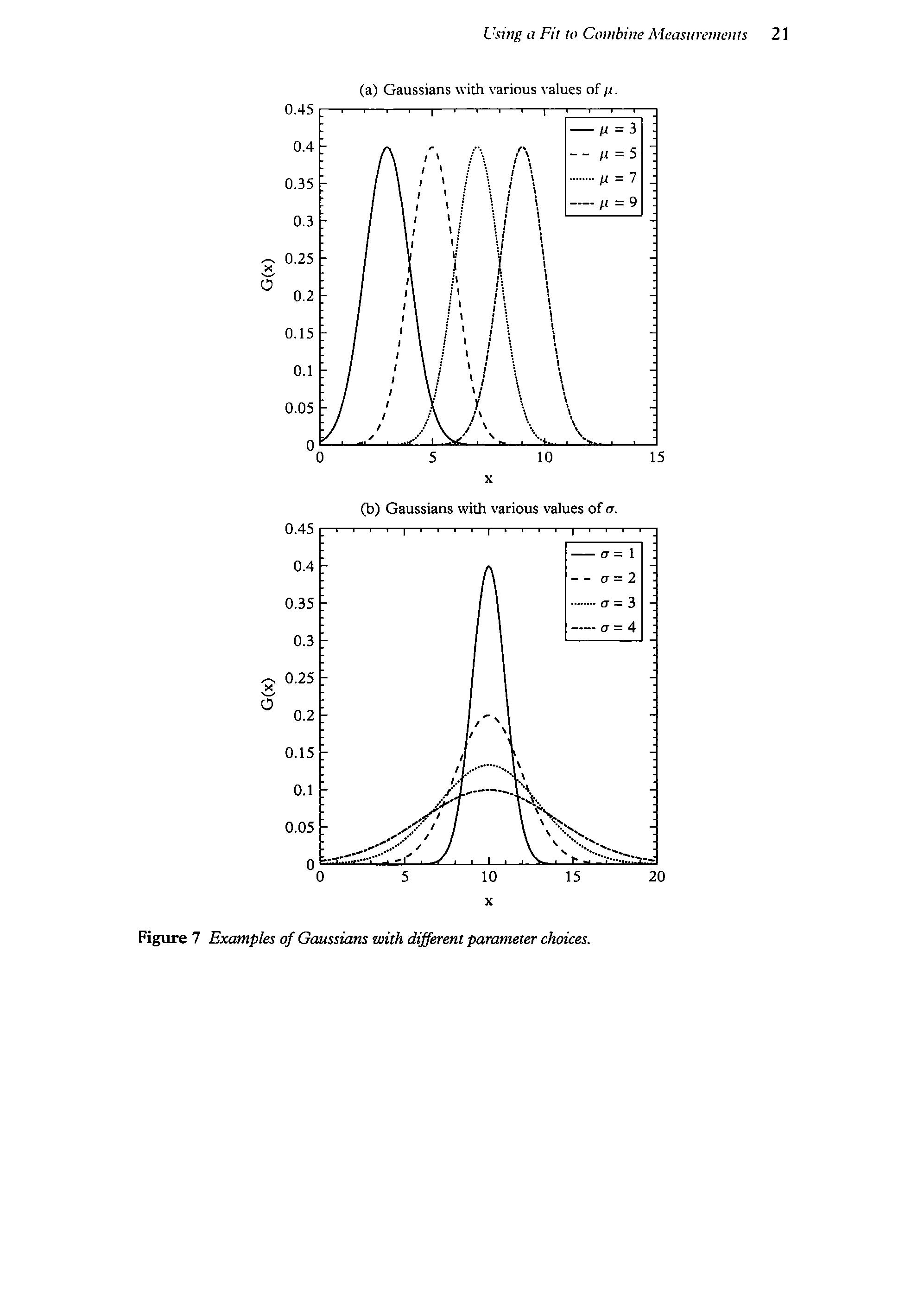
The Gaussian is defined by two parameters: the mean (yu, which shifts the curve as in figure 7a) and the standard deviation (0, which makes the argumentofthe exponential dimensionless and defines the spread of the curveas in figure 7b). That s it. Sometimes people give other reasons why the Gaussian should be the curve that describes the uncertainties of our measurements (notably including Gausshimself). In ouropinion,the mostconvincing reasoning is the Central Limit Theorem itself.
3.3. Using a Fit to Combine Measurements
The goal ofa fit is to find the line that is closest to all of the points. In the case of a linear model with no intercept (y(0) =0), the goal is to find the slope, A,
2 If your jaw hasn t dropped yet, consider again how remarkableit is that, starting with random variables drawn from any distribution (even a flat uniform distribution), summing them,andplotting the distribution ofthe sums, you end up with a Gaussian!
(a) Gaussians with variousvalues of yz. 0.45, a or 7
(b) Gaussians with various values ofo. 0.45 ooo 7
Figure 7 Examples ofGaussians with differentparameter chotces.
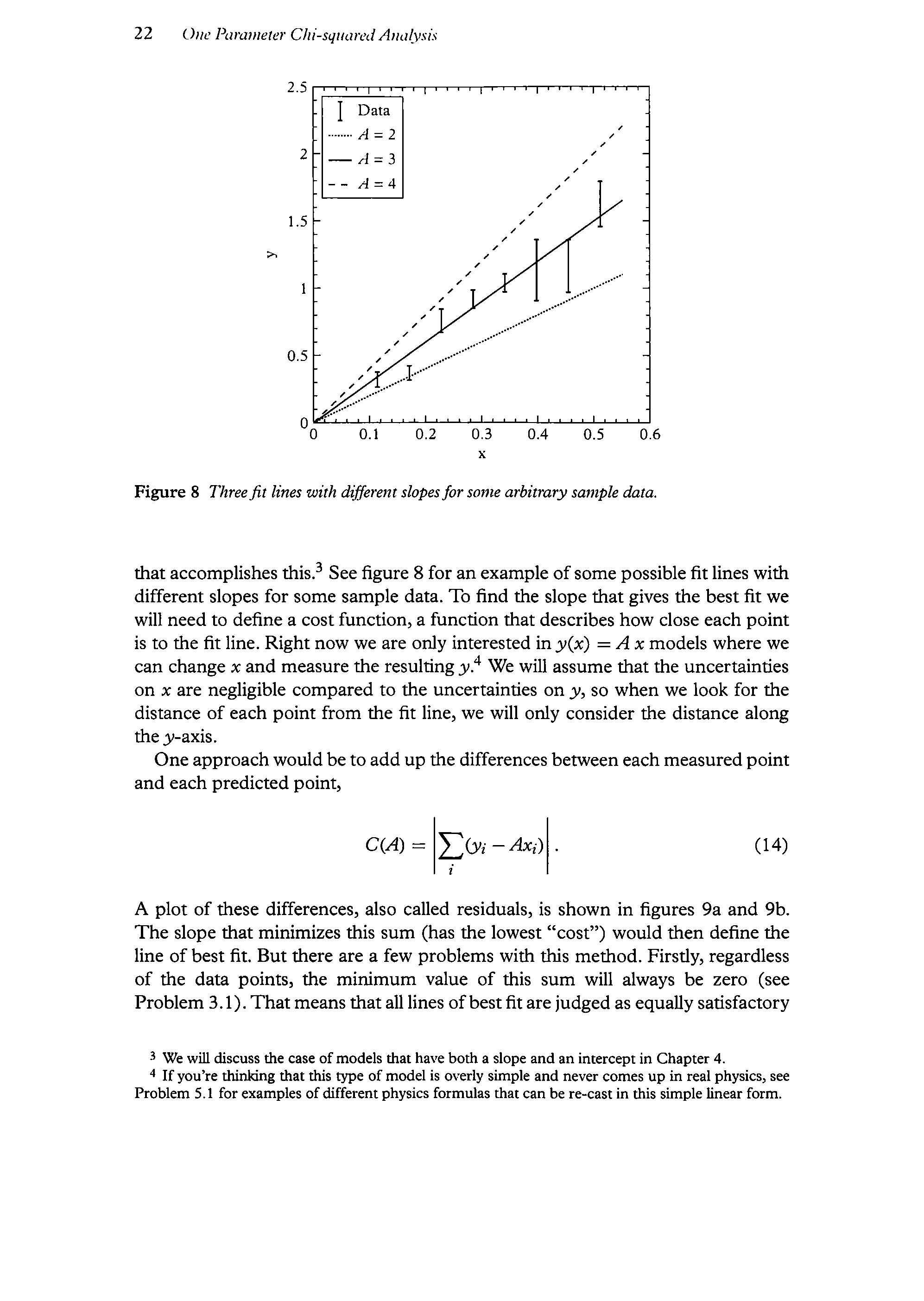
Figure 8 Threefit lines with different slopesforsome arbitrary sample data.
that accomplishesthis.? See figure 8 for an example ofsomepossiblefit lines with different slopes for some sample data. To find the slope that gives the best fit we will need to define a cost function, a function that describes how close each point is to the fit line. Right now weare only interested iny(x) = A x models where we can change x and measuretheresulting y.4 We will assumethat the uncertainties on x are negligible compared to the uncertainties on y, so when we look for the distance of each point from thefit line, we will only consider the distance along they-axis.
One approach would be to add up the differences between each measured point and each predicted point,
C(A) = |5° 0% - Ax}. (14)
A plot of these differences, also called residuals, is shown in figures 9a and 9b. The slope that minimizes this sum (has the lowest cost ) would then define the line of best fit. But there are a few problems with this method.Firstly, regardless of the data points, the minimum value of this sum will always be zero (see Problem 3.1). That meansthatall lines ofbestfit are judged as equally satisfactory
3 We will discuss the case ofmodels that have both a slope and an intercept in Chapter 4.
4 Ifyou re thinking that this type of modelis overly simple and never comesup in real physics, see Problem 5.1 for examples ofdifferent physics formulas that can be re-castin this simple linear form.