Oxford University Press is a department of the University of Oxford. It furthers the University’s objective of excellence in research, scholarship, and education by publishing worldwide. Oxford is a registered trade mark of Oxford University Press in the UK and certain other countries.
Published in the United States of America by Oxford University Press 198 Madison Avenue, New York, NY 10016, United States of America.
All rights reserved. No part of this publication may be reproduced, stored in a retrieval system, or transmitted, in any form or by any means, without the prior permission in writing of Oxford University Press, or as expressly permitted by law, by license, or under terms agreed with the appropriate reproduction rights organization. Inquiries concerning reproduction outside the scope of the above should be sent to the Rights Department, Oxford University Press, at the address above.
You must not circulate this work in any other form and you must impose this same condition on any acquirer.
Library of Congress Cataloging-in-Publication Data
Names: Racine, Jeffrey Scott, 1962- author.
Title: Reproducible econometrics using R / Jeffrey S. Racine.
Description: New York : Oxford University Press, [2019] | Includes bibliographical references and index.
Identifiers: LCCN 2018024219 (print) | LCCN 2018035264 (ebook) ISBN 9780190900670 (UPDF) ISBN 9780190900687 (EPUB) ISBN 9780190900663 (hardcover : alk. paper)
Subjects: LCSH: Econometrics. Open source software.
Classification: LOO HB139 (ebook) LOO HB139 .R3293 2019 (print) DDC 330.0285/5133—dc23
LC record available at https://lccn.loc.gov/2018024219
9 8 7 6 5 4 3 2 1
Printed by Sheridan Books, Inc., United States of America
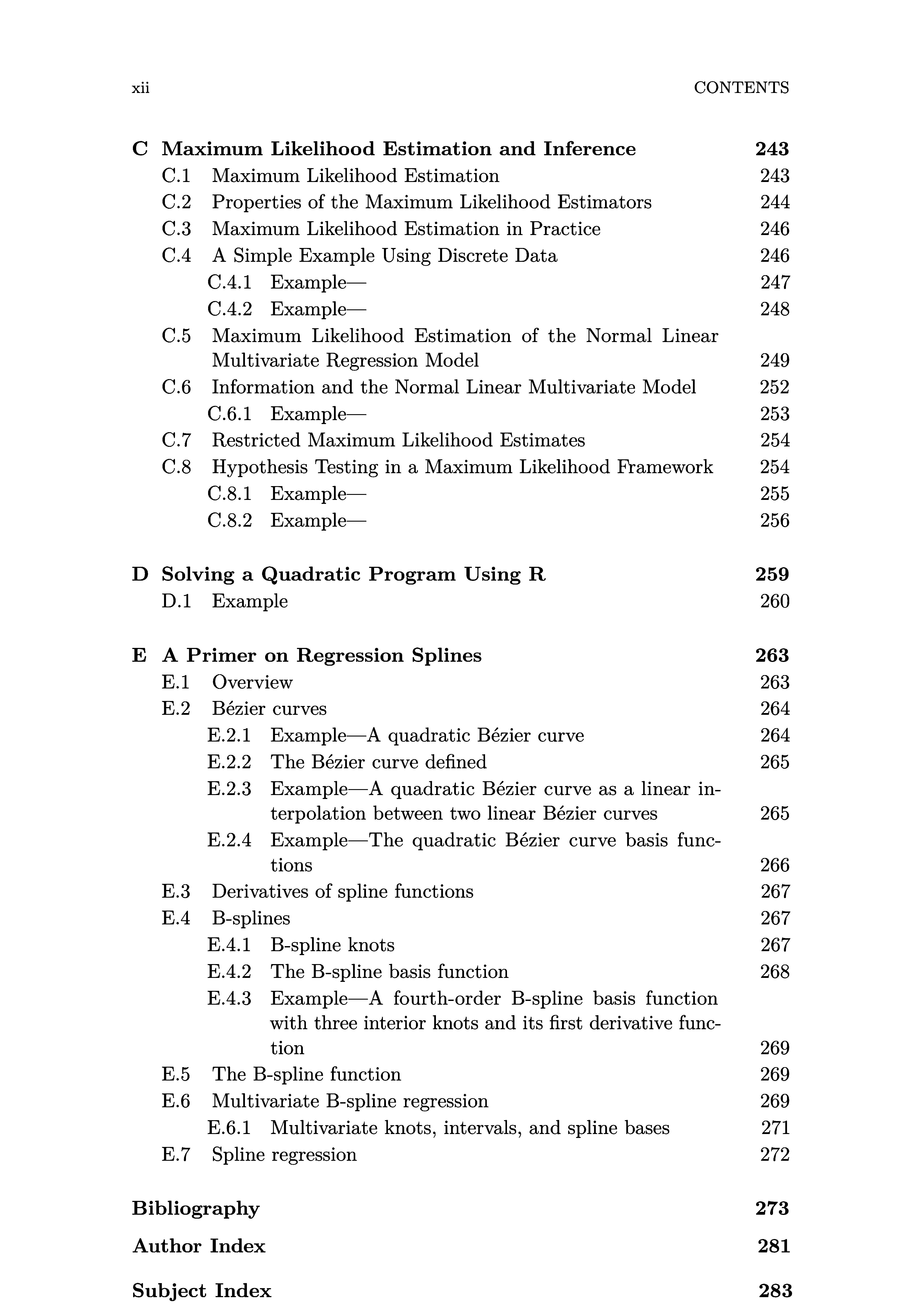
List of Tables xiii
List of Figures
Preface
About the Companion Website
I Linear Time Series Methods
R and Time Series Analysis
Overview
Some Useful R Functions for Time Series Analysis
1 Introduction to Linear Time Series Models
1.1 Overview 1.2 Time Series Data Patterns in Time Series Stationary versus Non-Stationary Series Examples of Univariate Random Processes
cnii>oo
1.6 1.7
1.5.1 White Noise Processes
1.5.2 Random Walk Processes Characterizing Time Series
1.6.1 The Autocorrelation Function
1.6.2 The Sample Autocorrelation Function
1.6.3 Non-Stationarity and Differencing Tests for White Noise Processes
1.7.1 Individual Test for H0: pk = 0—Bartlett’s Test
1.7.2 JointTestforH0:p1-0fip2=0fi---fipk=0— Ljung & Box’s Test
1.7.3 A Simulated Illustration—Testing for a White Noise Process
1.7.4 A Simulated Illustration—White Noise Tests when the Series is a Random Walk Process
2 Random Walks, Unit Roots, and Spurious Relationships 3
Overview
Properties of a Random Walk
Classical Least Squares Inference and Random Walks 2.1
The Autocorrelation Function for a Random Walk
Classical Least Squares Estimators and Random Walks
2.5.3
2.6
2.7
Cross-Section (I.I.D. Data) Monte Carlo Time Series (Random Walk) Monte Carlo Time Series (Random Walk with Drift) Monte Carlo
Unit Root Tests
2.6.1
Testing for a Unit Root in Spot Exchange Rates
Random Walks and Spurious Regression
3 Univariate Linear Time Series Models
3.1 Overview
3.2 Moving Average Models (MA(q))
3.2.1
3.2.2
3.2.3
3.2.4 3.2.5
3.2.6
3.2.7
3.2.8
3.2.9
3.3
Structure of MA(q) Processes
Example—Residential Electricity Sales Properties of MA(q) Processes
Stationarity of MA(q) Processes
The Autocorrelation Function and Identification of MA(q) Processes
Forecasting MA(q) Processes
Forecasting MA(q) Processes Assuming the cT_,- and the 9, are Known
Forecasting MA(q) Processes when the cT_,; and the 6,; are Estimated
Forecasting MA(q) Processes in the Presence of a Trend
Autoregressive Models (AR(p))
Structure of AR(p) Processes
Example—Residential Electricity Sales Properties of AR(p) Processes
Stationarity of AR(p) Processes
Invertiblity of Stationary AR(p) Processes
Identification of AR(p) Processes—The Partial Autocorrelation Function
3.3.7 3.3.8
3.3.9
Forecasting AR(p) Processes
Forecasting AR(p) Processes when the Parameters Q57; are Unknown
Forecasting AR(p) Processes in the Presence of a Trend
3.4 Non-Seasonal Autoregressive Moving Average Models (ARMA(P,q))
3.5 3.6 3.7
3.4.1 Structure
Non-Seasonal Autoregressive Integrated Moving Average Models (ARIMA(p, d, q))
3.5.1
3.5.2
3.5.3
3.5.4
3.5.5
3.5.6
3.5.7
3.5.8
3.5.9
Structure
Stationarity of ARIMA(p, d, q) Models Identification of ARIMA(p, d, q) Processes Estimation of ARIMA(p, d, q) Processes Forecasting ARIMA(p, d, q) Processes Trends, Constants, and ARIMA(p, d, q) Models Model Selection Criteria, Trends, and Stationarity Model Selection via auto arima() Diagnostics for ARIMA(p, d, q) Models
Seasonal Autoregressive Integrated Moving Average Models (AR1MA(P,d,q)(P,D,Q)m)
3.6.1
3.6.2
Example—Modelling and Forecasting European Quarterly Retail Trade Example—Modelling Monthly Cortecosteroid Drug Sales
ARIMA(p, d, q)(P, D, Q)m Models with External Predictors
3.8 Assessing Model Accuracy on Hold-Out Data
Problem Set II
Robust Parametric Inference
The Bootstrap and the Jackknife Overview Some Useful R Functions for Data-Driven Inference
4
Robust Parametric Inference Overview
Analytical Versus Numerical, i.e., Data-Driven, Procedures
4.2.1
4.2.2 Drawbacks of the Analytical Approach
An Illustrative Example—Testing for a Unit Root Alternatives to Analytical Approaches
4.3.1 Motivating Example—Compute the Standard Error of X
An Introduction to Efron’s Bootstrap
4.4.1
4.4.2 Bootstrapping a Standard Error for the Sample Mean Bootstrap Implementations in R
Jackknifing—Background and Motivating Example Jackknife and Bootstrap Estimates of Bias To Bootstrap or Jackknife?
4.11.1 Example—Nonparametric Confidence Intervals for the Population Mean
4.12 Bootstrap Inference
4.12.2 Generating 9* Under the Null
4.12.1 How Many Bootstrap Replications? PPR
12.3 Example—The Two-Sample Problem
12.4 Example—Regression-Based Bootstrap Inference
12.5 Example—Unit Root Testing
5 Robust Parametric Estimation
5.1 Overview
5.2 Robust Estimation Basics
5.2.1
5.2.2
5.2.3
5.2.4
5.2.5 Outlier Breakdown Point Sensitivity Curve Contamination Neighborhoods Influence Function
5.3 Unmasking Univariate Outliers
5.3.1
5.3.2
5.3.3
5.3.4
5.3.5
5.3.6
5.3.7
5.3.8
L1 and L2-norm Estimators of Central Tendency Robustness versus Efliciency M-Estimator Methods
Optimal Robustness
Huber’s M-Estimator of Location—A More Efficient Robust Location Estimator than the Median Rousseeuw and Croux’s Qn Estimator of Scale—A More Efficient Robust Scale Estimator than MADT, M-Estimators of Scale Unmasking Univariate Outliers—The three-sigma edit rule
7.2 Classification Analysis and Support Vector Machines
7.2.1 The Confusion Matrix
7.2.2 Support Vector Machines
7.3 Nonparametric Kernel Regression
A R, RStudio, TeX, and Git
A.1 Installation of R and RStudio Desktop
A.2 What is R?
A.2.1 R in the News
A.2.2 Introduction to R
A.2.3 Econometrics in R
A.3 What is RStudio Desktop?
A.3.1 Introduction to RStudio
A.4 Installation of TeX
Installation of Git
B.1 Source Code (R Markdown) for this Document
B.2 R, RStudio, TeX and git
B.3 What is R Markdown?
B.4 Creating a New R Markdown Document in RStudio
B.5 Including R Results in your R Markdown Document
B.6 Reading Data from a URL
B.7 Including Plots
B.8 Including Bulleted and Numbered lists
B.9 Including Tables
B 10 Including Verbatim, i.e., Freeform, Text
Typesetting Mathematics
C.5
C.6
E.2.2
E.2.3
E.4.1
E.4.3
E.5
E.6.1
List of Tables
1.1 ACF Summary (White Noise).
1.2 ACF Summary (Random Walk).
2.1 Critical Values for the Dickey Fuller Test H0: 71 = 0 (default, for a regression with no intercept [constant] nor time trend). Rows Present Critical Values for Different Sample Sizes, Columns Present Quantiles.
3.2 BIC Model Selection Criterion Values for Four Candidate Models Based on a Trend Stationary AR(1) Process and a Random Walk with Drift (smaller values are better).
3.3 Canadian Lynx Forecasts.
3.4 European Quarterly Retail Trade Forecasts.
3.5 Australian Monthly Cortecosteroid Drug Sales Forecasts.
3.6 Model Summary.
3.7 Forecasted Deaths/Injuries in 1985 With and Without Compulsory Seatbelt Laws.
4.1 Jackknife and Bootstrap Bias Estimation.
4.2 Bootstrap Size and Power.
4.3 Bootstrap and Tabulated Critical Values for the Augmented Dickey-Fuller Statistic (n=100) with trend— argument following the hyphen (B=Bootstrap, DF=DickeyFuller, M=MacKinnon).
4.4 Bootstrap Unit Root Test, Stationary ARMA(2,2), n=100.
6.1 Mean MSE and Ranking of MSE Performance (k = 6 is the oracle model).
6.2 Model Selection Proportion Among the Candidate Models (k = 6 is the oracle model).
6.3 Mean MSE and Ranking of MSE Performance (k = 4 is the oracle model).
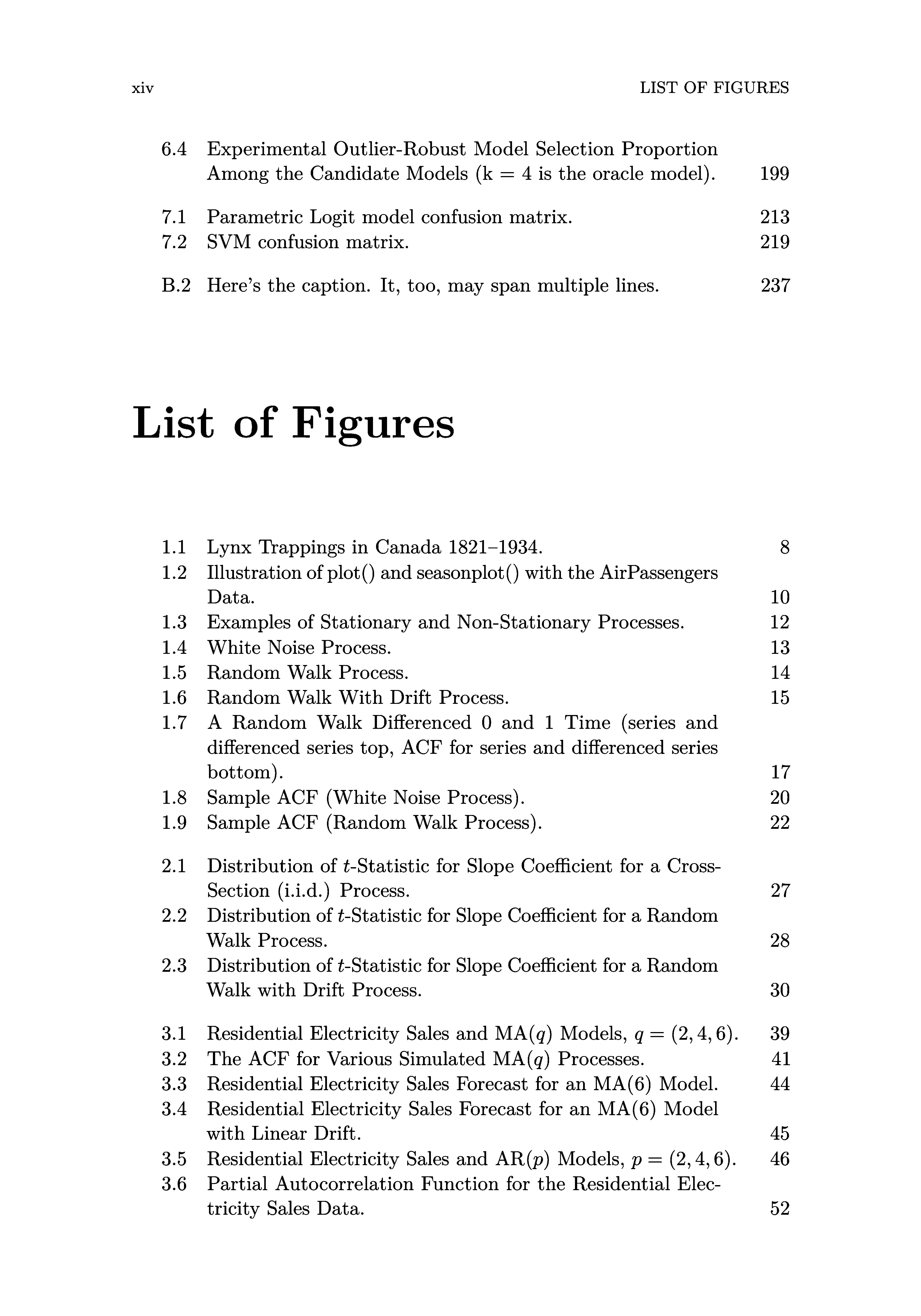
Experimental Outlier-Robust Model Selection Proportion Among the Candidate Models (k = 4 is the oracle model).
Parametric Logit model confusion matrix. SVM confusion matrix.
Here’s the caption. It, too, may span multiple lines.
List of Figures
Lynx Trappings in Canada 1821-1934.
Illustration of plot() and seasonplot() with the AirPassengers Data.
Examples of Stationary and Non-Stationary Processes.
White Noise Process.
Random Walk Process.
Random Walk With Drift Process.
A Random Walk Differenced 0 and 1 Time (series and differenced series top, ACF for series and differenced series bottom).
Sample ACF (White Noise Process).
Sample ACF (Random Walk Process).
Distribution of t-Statistic for Slope Coefficient for a CrossSection (i.i.d.) Process.
Distribution of t-Statistic for Slope Coefficient for a Random Walk Process.
Distribution of t-Statistic for Slope Coefficient for a Random Walk with Drift Process.
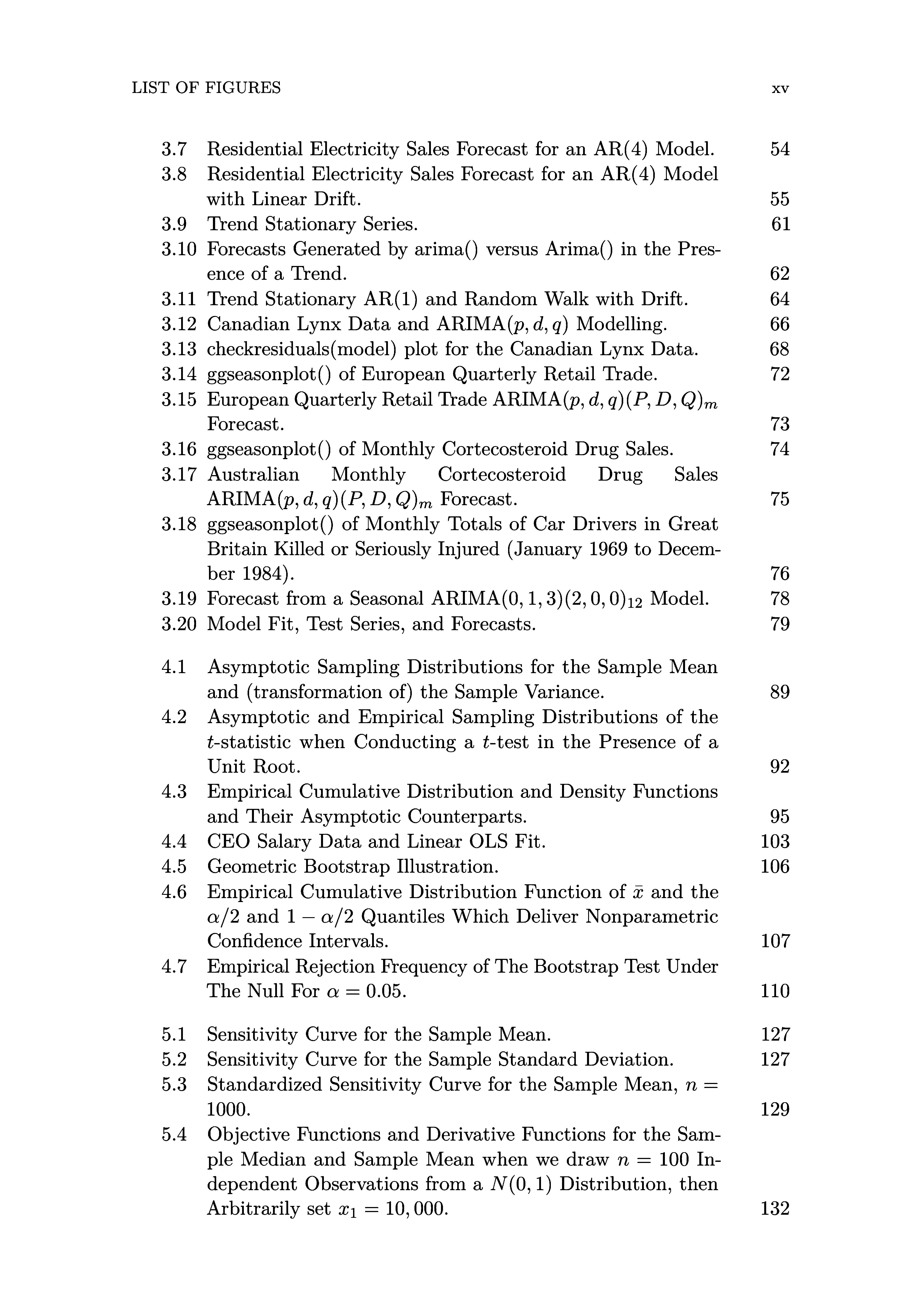
ggseasonplot() of Monthly Cortecosteroid Drug Sales.
Australian Monthly Cortecosteroid Drug Sales ARIMA(p, d, q)(P, D, Q)m Forecast.
ggseasonplot() of Monthly Totals of Car Drivers in Great Britain Killed or Seriously Injured (January 1969 to December 1984).
Forecast from a Seasonal ARIMA(0, 1, 3)(2, 0, 0)12 Model.
Model Fit, Test Series, and Forecasts.
Asymptotic Sampling Distributions for the Sample Mean and (transformation of) the Sample Variance.
Asymptotic and Empirical Sampling Distributions of the t-statistic when Conducting a t-test in the Presence of a Unit Root.
Empirical Cumulative Distribution and Density Functions and Their Asymptotic Counterparts.
CEO Salary Data and Linear OLS Fit.
Geometric Bootstrap Illustration.
Empirical Cumulative Distribution Function of 5: and the oz/2 and 1 - 0:/2 Quantiles Which Deliver Nonparametric Confidence Intervals.
Empirical Rejection Frequency of The Bootstrap Test Under The Null For 04 = 0.05.
Sensitivity Curve for the Sample Mean.
Sensitivity Curve for the Sample Standard Deviation. Standardized Sensitivity Curve for the Sample Mean, n = 1000.
Objective Functions and Derivative Functions for the Sample Median and Sample Mean when we draw n 100 Independent Observations from a N(0, 1) Distribution, then Arbitrarily set 51:1 = 10, 000.
5.5 Huber’s p(u) Function and the L1 Function
5.6 Huber’s ¢(u) Function and the L1 Derivative Function sgn(u)
5.7 Density Histograms of Copper Content With (left) and Without (right) Outlier.
5.8
5.9
Bisquare pC(u) Function for c = 1.0 and c = 0.5, and the L1
Objective Function
Bisquare ¢C('u.) Function for c = 1.0 and c = 0.5, and the L1 Derivative Function sgn(-).
Normal Quantile-Quantile Plot.
Belgian Telephone Data.
Classical Mahalanobis Distance for Belgian Telephone Data.
Tolerance Ellipse (97.5%) for the Belgian Telephone Data.
Robust Mahalanobis Distance for the Belgian Telephone Data.
DGP and Data (No Outliers).
Outlier in the Y Direction.
DGP and Data (No Outliers).
Outlier in the X Direction.
An Example of a Good Leverage Point.
An Example of a Bad Leverage Point. OLS Fit with a Bad Leverage Point.
OLS Residuals with a Bad Leverage Point.
Hat Matrix Diagonals (hit).
Studentized Residuals.
The robust LTS estimator versus the OLS estimator with an Outlier in the X direction.
Belgian Telephone Data with LTS and OLS Estimate. 5.26 5.27 5.28
The robust LTS estimator versus the OLS estimator with an Outlier in the Y direction.
Standardized LTS Residuals for the Belgian Telephone Data.
6.1 Data, g(a:), and Linear Model Fit (Top), dg(a:)/da: and 61 (Bottom).
6.2 Monte Carlo DGP.
6.3 Model Selection, Averaging, and Assertion with 10 Candidate Models (orthogonal polynomials of order 1-10).
6.4 Model Averaging Illustration (true DGP is y,- = 1 293% + 9:732 + e,;, correctly specified model is not among the set of candidate models).
6.5 A Quadratic Bézier Curve.
6.6 The Quadratic Bézier Curve Bases.
6.7 Experimental Outlier-Robust Model Selection, Averaging, and Assertion with 8 Candidate Models (orthogonal polynomials of order 1-8).
A Simple Illustration With Two Covariates, X1 and X2 and a Binary Response Y € D = {A, B}, and Three Potential Boundaries.
A Simple Illustration With Two Covariates, X1 and X2 and a Binary Response Y € D = {A,B}, One Potential Boundary and its Margins.
A Simple Illustration With Two Covariates, X1 and X2 and a Binary Response Y € D = {A,B}, One Potential Boundary, The Margin (perpendicular distance between the leftmost dashed line and the solid line), and the Empty Region.
A Simple Illustration With Two Covariates, X1 and X2 and a Binary Response Y € D = {A, B}, the Optimal Boundary, Margins, and the Support Vectors (points appearing in a circle). Note That There Is One Missclassified Observation (the support vector, i.e., the circled A that lies to the left of the boundary hence is incorrectly classified as a B).
A Simple Model-Free Nonparametric Conditional Mean Estimator (the true conditional mean is the solid line, the dark circles the estimates).
Weighted Least Squares Construction of the Local Linear Estimator and its Derivative.
Using the npreg() Function to Compute the Local Linear Estimator and its Derivative.
Likelihood Function for Binomial Sample :1: = {1, 1, 0}.
Likelihood Function for Binomial Sample :1: {1, 0, 0}. Power Curve for a Likelihood Ratio Test of Significance.
A Quadratic Bézier Curve.
Quadratic Bézier curve basis functions. Third degree B-spline with three interior knots along with its first derivative.
Preface
The increasing recognition of the importance of reproducibility and the recent availability of new tools to facilitate reproducibility were the inspiration for this project. While these developments have yet to be widely embraced by the profession, it is my belief that they will be commonplace in the not too distant future.
With the release of a set of free and open source tools on December 6 2016 (the official release of R Markdown (Allaire et al., 2017)), I decided to incorporate them into a course that I taught in the Winter of 2017. Rather than teach a traditional course from any one of the excellent textbooks that exist, I decided to cover a set of topics that I felt would benefit future researchers but to do so with an emphasis on reproducibility, and was not aware of any one text that covers the set of topics I wished to cover from the perspective I envisioned. Furthermore, I wanted the students to be critical and to confront model uncertainty and the lack of robustness of many techniques that they have been taught, while providing sound alternatives. I therefore decided to create a set of notes for the students.
When I taught the Winter 2017 course, the first order of business was to introduce the students to R and R Markdown, and have them install R, R Markdown, TeX and git on their laptops and bring their laptop to the second class to ensure that their installations were working correctly. Their first assignment and all subsequent work exploited this framework and they immediately appreciated the benefits of working with one document only that contained their narrative and analysis. They wrote their term paper in R Markdown and rendered it as a PDF and presented their work by writing slides in R Markdown and rendering them in LaTeX Beamer PDF format. The installation instructions and the introduction to R Markdown that I created for the students form the basis for appendices A and B of this book. These appendices contain a number of links and pointers to helpful sites that will get the novice practitioner up and running; see also Racine (2018) that provides a more detailed overview of replicability and reproducibility in this framework which too arose out of the course.
These notes were written as the course progressed and were made available to students each week in real-time, which simply would not have been possible
without the use of R Markdown. The R code underlying every example was also made available to them (this is stripped from the Markdown document with a simple command in R, knitr: :purl("foo .R.md")), and slides written in R Markdown generated from the chapters were rendered in LaTeX Beamer (the course website was also created using R Markdown). At the end of the course I had a fairly complete manuscript.
When I began the course, my intention was to create a set of notes for the students. But as the course unfolded, it dawned upon me that this project might be useful to a broader audience, which led to the book in its current form. Since all assignments were written in R Markdown with answers embedded so that I could print either the questions or both questions and answers, this formed the basis for a solutions manual. At the end of the course I had a reproducible manuscript, the students were well versed in reproducible econometric methods, and it is my hope that the combination of reproducible tools, a book to guide instructors, all R code underlying every example, a set of slides that can be modified by the instructor for their purposes, plus a solutions manual including potential exam questions and answers might be something of value to the broader community.
This book is intended for students studying Econometrics who are interested in leveraging recent developments in reproducible research. It relies on freely available open source tools such as R, RStudio, TeX, BibTeX, and git. Detailed appendices guide the reader through the process of installation and adoption of these tools, while the topics covered in the five parts are topics that every student ought to be familiar with.
The material consists of five parts:
o Linear Time Series Methods
0 Resampling Methods
0 Outlier-Resistant Methods
o Model Uncertainty Methods
o Advanced Topics (Support Vector Machines and Nonparametric Regression)
This project would not have been possible without the remarkable contributions from an army of individuals whose efforts support and sustain the open source revolution that is the R Project for Statistical Computing (R Core Team, 2017) and the Integrated Development Environment RStudio (RStudio Team, 2016). The list of contributors is exceedingly large, far to large to attempt here, but I do want to acknowledge my deepest gratitude their efforts.
A substantial amount of the material covered in this book is based on lecture notes that I compiled over the past few decades while teaching various courses. I would like to acknowledge (but not implicate) the authors of the main texts that influenced my thinking.
o Time series—the 1991 version of Pindyck and Rubinfeld (1998), the
1995 version of Enders (2015), and Hyndman and Athanasopoulos’ text (Hyndman and Athanasopoulos, 2018) and their R package fpp2 (I am also extremely grateful to Rob Hyndman for patiently explaining the inner workings of certain functions in his forecast (Hyndman, 2017b) package).
0 Resampling—the texts of Efron (1984) and Efron and Tibshirani (1993)
0 Robustness—the texts of Rousseeuw and Leroy (2003) and Maronna et al. (2006).
0 Model uncertainty—the text of Claeskens and Hjort (2008) (I have also been strongly influenced by the work of Bruce Hansen, e.g., Hansen (2007)).
o Maximum likelihood Appendix—the text of Silvey (1975). Finally, I would be remiss if I did not thank my spouse, Jennifer, and son, Adam, for enduring my obsession with this project during the Winter 2017 semester.
This is an R Markdown/bookdown document. R Markdown/bookdown is a simple formatting syntax for authoring HTML, PDF, LaTeX, epub, MOBI, and MS Word documents in RStudio. For more details on using R Markdown and bookdown see http://rmarkdown.rstudio.com and https: //bookdown.org/yihui/bookdown.
About the Companion Website
www.oup.com/us/reproducibleeconometricsusingr
Oxford has created a website to accompany Reproducible Econometrics Using R. Instructors are encouraged to consult this resource. If you are an instructor and would like to access this section, please email Custserv.us@ oup.com with your course information to receive a password.
Part I
Linear Time Series Methods
R and Time Series Analysis
Overview
This document uses R (R Core Team, 2017) for data analysis. Readers familiar with other statistical software yet unfamiliar with R might assume that certain functions in R are carbon copies of their counterparts elsewhere. However, this may not be the case, particularly in the time series domain. There are some important points that you ought to be aware of when using R for time series analysis:
o In R, there are numerous datatypes (numeric, factor, ts and so forth)
o For time series, there is the ts () function which casts a data vector as a time series object (type numeric is the default data type in R)
o This ts datatype can be manipulated using specialized time series functions such as diffinv(foo), decompose(foo) and lag(foo,-1) where foo is a time series object
o plot() and many functions will automatically recognize time series objects and plot them accordingly, i.e., in the time domain
0 However, not all methods are designed to manipulate time series objects (the standard function for linear regression in R, lm(), does not by way of illustration), so beware
o If by chance you did wish to use classical least squares regression methods for modelling time series objects and conducting hypothesis tests (not a good idea as we shall see), you could use the R package dyn (Grothendieck, 2017) and the function dyn$lm() instead of lm() (you will have to install the dyn package first)
o For a brief overview of and introduction to time series methods in R see Quick R Time Series (http://www.statmethods.net/advstats/ timeseries.html)
0 Rob Hyndman and George Athanasopoulos have created an online introductory text that provides numerous non-technical illustrations: see Forecasting: Principles and Practice (https://www.otexts.org/fpp2) and the R package fpp2 (Hyndman, 2018) that accompanies their text
0 See also the CRAN Task View: Time Series Analysis (https://cran. r-project.org/web/views/TimeSeries.html)
This document incorporates R code that is routinely used for the analysis of time series data, among others. It is important that you study the code and understand how it works so that you can modify it to suit your own needs.
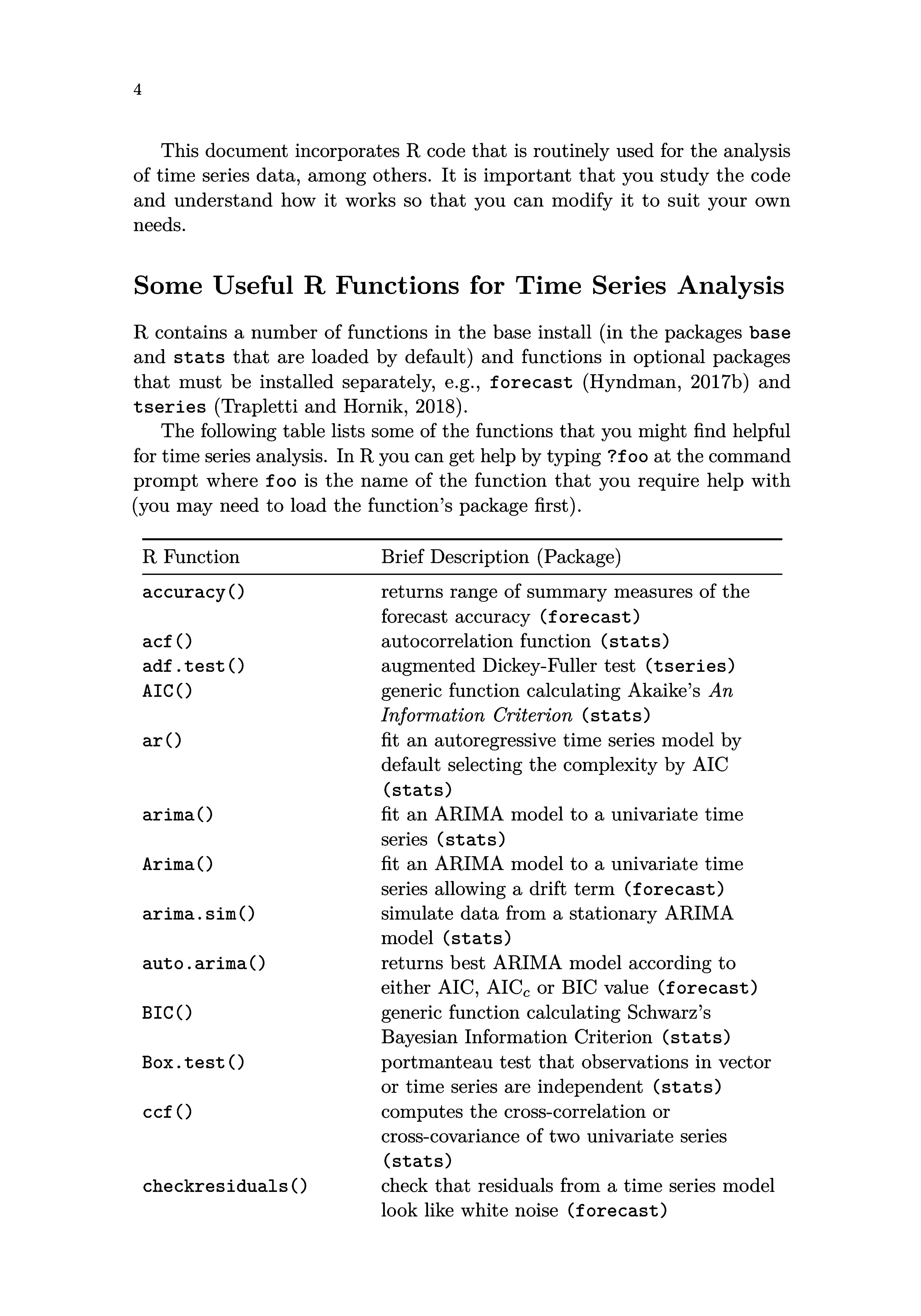
Some Useful R Functions for Time Series Analysis
R contains a number of functions in the base install (in the packages base and stats that are loaded by default) and functions in optional packages that must be installed separately, e.g., forecast (Hyndman, 2017b) and tseries (Trapletti and Hornik, 2018).
The following table lists some of the functions that you might find helpful for time series analysis. In R you can get help by typing ?foo at the command prompt where foo is the name of the function that you require help with (you may need to load the function’s package first).
R Function Brief Description (Package) accuracy() acf() adf.test() AIc() ar() arima() Arima() arima.sim() auto.arima() BIC() Box.test() ¢¢£(>
checkresiduals()
returns range of summary measures of the forecast accuracy (forecast) autocorrelation function (stats) augmented Dickey-Fuller test (tseries) generic function calculating Akaike’s An Information Criterion (stats)
fit an autoregressive time series model by default selecting the complexity by AIC (stats)
fit an ARIMA model to a univariate time series (stats)
fit an ARIMA model to a univariate time series allowing a drift term (forecast) simulate data from a stationary ARIMA model (stats) returns best ARIMA model according to either AIC, AICC or BIC value (forecast) generic function calculating Schwarz’s Bayesian Information Criterion (stats) portmanteau test that observations in vector or time series are independent (stats) computes the cross-correlation or cross-covariance of two univariate series (stats)
check that residuals from a time series model look like white noise (forecast)
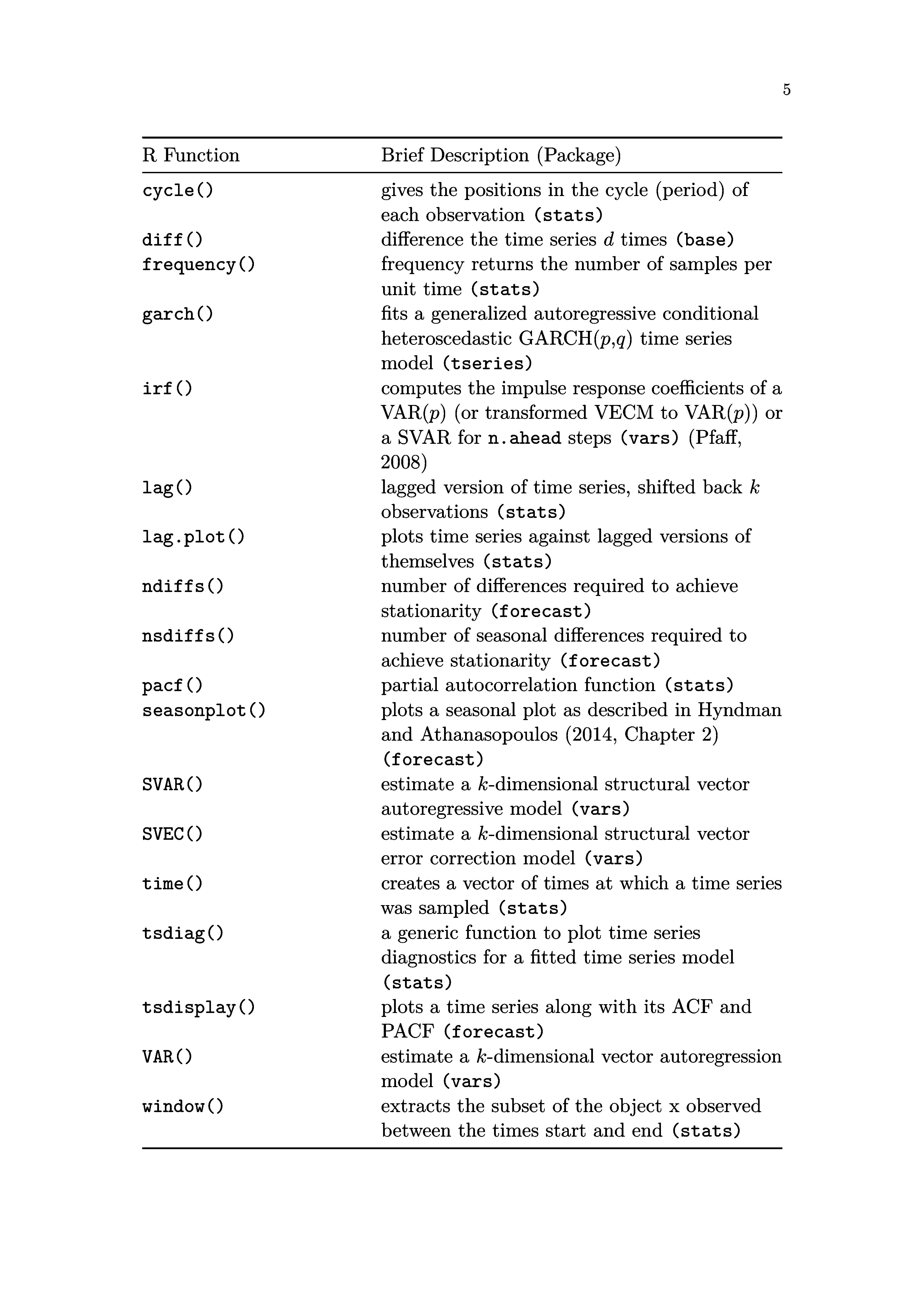
R Function
Brief Description (Package) cycle()
diff() frequency()
garch()
irf() lag()
lag.plot() ndiffs() nsdiffs()
pacf() seasonplot()
SVAR() svEc() time()
tsdiag()
tsdisplay() VAR() window()
gives the positions in the cycle (period) of each observation (stats) difference the time series d times (base) frequency returns the number of samples per unflztnne (stats)
fits a generalized autoregressive conditional heteroscedastic GARCH(p,q) time series rnodel(tseries) computes the impulse response coefficients of a VAR(p) (or transformed VECM to VAR(p)) or a SVAR for n. ahead steps (vars) (Pfaff, 2008)
lagged version of time series, shifted back k observations (stats) plots time series against lagged versions of themselves (stats) number of differences required to achieve stationarity (forecast) number of seasonal differences required to achieve stationarity (forecast) partial autocorrelation function (stats) plots a seasonal plot as described in Hyndman and Athanasopoulos (2014, Chapter 2) (forecast)
estimate a I4:-dimensional structural vector autoregressive model (vars) estimate a I4:-dimensional structural vector error correction model (vars) creates a vector of times at which a time series was sampled (stats) a generic function to plot time series diagnostics for a fitted time series model (stats)
plots a time series along with its ACF and PACF (forecast)
estimate a k-dimensional vector autoregression Inodel(vars) extracts the subset of the object x observed between the times start and end (stats)