Essential statistics for data science: a concise crash course 1st edition mu zhu 2024 scribd downloa by Education Libraries

Essential Statistics for Data Science: A Concise Crash Course 1st Edition

Mu Zhu

Visit to download the full and correct content document: https://ebookmass.com/product/essential-statistics-for-data-science-a-concise-crashcourse-1st-edition-mu-zhu/

More products digital (pdf, epub, mobi) instant download maybe you interests ...

Google Cloud Platform for Data Science: A Crash Course on Big Data, Machine Learning, and Data Analytics Services Dr. Shitalkumar R. Sukhdeve

https://ebookmass.com/product/google-cloud-platform-for-datascience-a-crash-course-on-big-data-machine-learning-and-dataanalytics-services-dr-shitalkumar-r-sukhdeve/

Python for Finance: A Crash Course Modern Guide: Learn Python Fast Bisette

https://ebookmass.com/product/python-for-finance-a-crash-coursemodern-guide-learn-python-fast-bisette/

Crash Course in Collection Development 2nd Edition

https://ebookmass.com/product/crash-course-in-collectiondevelopment-2nd-edition/

Crash Course Psychiatry 5th Edition Xiu Philip

https://ebookmass.com/product/crash-course-psychiatry-5thedition-xiu-philip/

Machine Learning for Signal Processing: Data Science, Algorithms, and Computational Statistics Max A. Little

https://ebookmass.com/product/machine-learning-for-signalprocessing-data-science-algorithms-and-computational-statisticsmax-a-little/

PYTHON PROGRAMMING: 3 MANUSCRIPTS CRASH COURSE CODING WITH PYTHON DATA SCIENCE. THE STEP BY STEP GUIDE FOR BEGINNERS TO MASTER SOFTWARE PROJECTS, ALGORITHMS, TRICKS AND TIPS Tacke

https://ebookmass.com/product/python-programming-3-manuscriptscrash-course-coding-with-python-data-science-the-step-by-stepguide-for-beginners-to-master-software-projects-algorithmstricks-and-tips-tacke/

Principles of Data Science - Third Edition: A beginner's guide to essential math and coding skills for data fluency and machine learning Sinan Ozdemir

https://ebookmass.com/product/principles-of-data-science-thirdedition-a-beginners-guide-to-essential-math-and-coding-skillsfor-data-fluency-and-machine-learning-sinan-ozdemir/

Winning with Data Science: A Handbook for Business Leaders Friedman

https://ebookmass.com/product/winning-with-data-science-ahandbook-for-business-leaders-friedman/

Data Science for Genomics 1st Edition Amit Kumar Tyagi

https://ebookmass.com/product/data-science-for-genomics-1stedition-amit-kumar-tyagi/

EssentialStatisticsfor DataScience

AConciseCrashCourse

Professor,UniversityofWaterloo

MUZHU

GreatClarendonStreet,Oxford,OX26DP, UnitedKingdom

OxfordUniversityPressisadepartmentoftheUniversityofOxford. ItfurtherstheUniversity’sobjectiveofexcellenceinresearch,scholarship, andeducationbypublishingworldwide.Oxfordisaregisteredtrademarkof OxfordUniversityPressintheUKandincertainothercountries ©MuZhu2023

Themoralrightsoftheauthorhavebeenasserted Allrightsreserved.Nopartofthispublicationmaybereproduced,storedin aretrievalsystem,ortransmitted,inanyformorbyanymeans,withoutthe priorpermissioninwritingofOxfordUniversityPress,orasexpresslypermitted bylaw,bylicenceorundertermsagreedwiththeappropriatereprographics rightsorganization.Enquiriesconcerningreproductionoutsidethescopeofthe aboveshouldbesenttotheRightsDepartment,OxfordUniversityPress,atthe addressabove

Youmustnotcirculatethisworkinanyotherform andyoumustimposethissameconditiononanyacquirer

PublishedintheUnitedStatesofAmericabyOxfordUniversityPress 198MadisonAvenue,NewYork,NY10016,UnitedStatesofAmerica

BritishLibraryCataloguinginPublicationData

Dataavailable

LibraryofCongressControlNumber:2023931557

ISBN978–0–19–286773–5

ISBN978–0–19–286774–2(pbk.)

DOI:10.1093/oso/9780192867735.001.0001

Printedandboundby CPIGroup(UK)Ltd,Croydon,CR04YY

LinkstothirdpartywebsitesareprovidedbyOxfordingoodfaithand forinformationonly.Oxforddisclaimsanyresponsibilityforthematerials containedinanythirdpartywebsitereferencedinthiswork.

ToEverestandMariana

PARTI.TALKINGPROBABILITY

PARTII.DOINGSTATISTICS

4.3Twomoredistributions

5.FrequentistApproach

5.1Maximumlikelihoodestimation

5.1.1Randomvariablesthatarei.i.d.

5.1.2Problemswithcovariates

5.2Statisticalpropertiesofestimators

6.BayesianApproach

6.A.1Metropolisalgorithm

6.A.2Sometheory

6.A.3Metropolis–Hastingsalgorithm

PARTIII.FACINGUNCERTAINTY

7.IntervalEstimation

7.1Uncertaintyquantification

7.1.1Bayesianversion

7.1.2Frequentistversion

7.2Maindifficulty

7.3Twousefulmethods

7.3.1Likelihoodratio

7.3.2Bootstrap

8.TestsofSignificance

8.1Basics

8.1.1Relationtointervalestimation

8.1.2Thep-value

8.2Somechallenges

8.2.1Multipletesting

8.2.2Sixdegreesofseparation

Appendix8.AIntuitionofBenjamini-Hockberg

PARTIV.APPENDIX

Prologue

Whenmyuniversityfirstlaunchedamaster’sprogramindatascienceafew yearsago,Iwasgiventhetaskofteachingacrashcourseonstatisticsfor incomingstudentswhohavenothadmuchexposuretothesubjectatthe undergraduatelevel—forexample,thosewhomajoredinComputerScience orSoftwareEngineeringbutdidn’ttakeanyseriouscourseinstatistics.

OurDepartmentofStatisticsformedacommittee,whichfiercelydebated whatmaterialsshouldgointosuchacourse.(Ofcourse,Ishouldmention thatourDepartmentofComputerSciencewasaskedtocreateasimilarcrash courseforincomingstudentswhodidnotmajorinComputerScience,and theyhadalmostexactlythesameheateddebate.)Intheend,aconsensuswas reachedthatthestatisticscrashcourseshouldessentiallybe“fiveundergraduatecoursesinone”,taughtinonesemesteratamathematicallevelthatis suitableformaster’sstudentsinaquantitativediscipline.

Atmostuniversities,thesefiveundergraduatecourseswouldtypicallycarry thefollowingtitles:(i)Probability,(ii)MathematicalStatistics,(iii)Regression,(iv)Sampling,and(v)ExperimentalDesign.ThismeantthatImust somehowthinkofawaytoteachthefirsttwocourses—ayear-longsequence atmostuniversities—injustabouthalfasemester,andatarespectablemathematicalleveltoo.Thisbookismypersonalanswertothischallenge.(While compressingtheotherthreecourseswaschallengingaswell,itwasmuchmore straightforwardincomparisonandIdidnothavetostrugglenearlyasmuch.)

Onemayaskwhywemustinsiston“arespectablemathematicallevel”.This isbecauseourgoalisnotmerelytoteachstudentssomestatistics;itisalso towarmthemupforothergraduate-levelcoursesatthesametime.Therefore, readersbestservedbythisbookarepreciselythosewhonotonlywanttolearn someessentialstatisticsveryquicklybutalsowouldliketocontinuereading relativelyadvancedmaterialsthatrequireadecentunderstandingandappreciationofstatistics—includingsomeconferencepapersinartificialintelligence andmachinelearning,forinstance.

Iwillnowbrieflydescribesomemainfeaturesofthisbook.Despitethelightningpaceandtheintroductorynatureofthetext,a verydeliberate attempt isstillmadetoensurethatthreeveryimportantcomputationaltechniques— namely,theEMalgorithm,theGibbssampler,andthebootstrap—areintroduced.Traditionally,thesetopicsarealmostneverintroducedtostudents

“immediately”but,forstudentsofdatascience,therearestrongreasonswhy theyshouldbe.Iftheprocessofwritingthisbookhasbeenaquest,thenitis notanexaggerationformetosaythatthisparticulargoalhasbeenitsHoly Grail.

Toachievethisgoal,agreatdealofcareistakensoasnottooverwhelm studentswithspecialmathematical“tricks”thatareoftenneededtohandledifferentprobabilitydistributions.Forexample,PartI, TalkingProbability,uses onlythree distributions—specifically,theBinomialdistribution,theuniform distributionon (0,1),andthenormaldistribution—toexplainalltheessential conceptsofprobabilitythatstudentswillneedtoknowinordertocontinuewiththerestofthebook.Whenintroducingmultivariatedistributions, onlytheircorrespondingextensionsareused,forexample,themultinomial distributionandthemultivariatenormaldistribution.

Then,twomuchdeliberatedsetsofrunningexamples—specifically,(i) Examples 5.2, 5.4, 5.5,+ 5.6 and(ii)Examples 6.2 + 6.3—arecraftedinPart II, DoingStatistics,whichnaturallyleadstudentstotheEMalgorithmandthe Gibbssampler,bothinrapidprogressionandwithminimalhustleandbustle.Theserunningexamplesalsouseonlytwodistributions—inparticular,the Poissondistribution,andtheGammadistribution—to“getthejobdone”.

Overall,precedenceisgiventoestimatingmodelparametersinthefrequentistapproachandfindingtheirposteriordistributionintheBayesian approach,beforemoreintricatestatisticalquestions—suchasquantifyinghow muchuncertaintywehaveaboutaparameterandtestingwhethertheparameterssatisfyagivenhypothesis—arethenaddressedseparatelyinPartIII, FacingUncertainty.It’snothardforstudentstoappreciatewhywemustalways trytosaysomethingfirstabouttheunknownparametersoftheprobability model—eitherwhattheirvaluesmightbeiftheyaretreatedasfixedorwhat theirjointdistributionmightlooklikeiftheyaretreatedasrandom;howelse canthemodelbeusefultousotherwise?!Questionsaboutuncertaintyand statisticalsignificance,ontheotherhand,aremuchmoresubtle.Notonlyare thesequestionsrelativelyuncommonforverycomplexmodelssuchasadeep neuralnetwork,whosemillionsofparametersreallyhavenointrinsicmeaningtowarrantasignificancetest,buttheyalsorequireauniqueconceptual infrastructurewithitsownidiosyncraticjargon(e.g.thep-value).

Finally,somemathematicalfacts(e.g.Cauchy–Schwarz),stand-aloneclassic results(e.g.James–Stein),andmaterialsthatmaybeskippedonfirstreading (e.g.Metropolis–Hastings)arepresentedthrough“mathematicalinserts”,“fun boxes”,andend-of-chapterappendicessoastoreduceunnecessarydisruptions totheflowofmainideas.

PARTI

TALKINGPROBABILITY

Synopsis: Thestatisticalapproachtoanalyzingdatabeginswithaprobability modeltodescribethedata-generatingprocess;that’swhy,tostudystatistics, onemustfirstlearntospeakthelanguageofprobability.

EminenceofModels

Theveryfirstpointtomakewhenwestudystatisticsistoexplainwhythe languageofprobabilityissoheavilyused.

Everybodyknowsthatstatisticsisaboutanalyzingdata.Butweareinterestedinmorethanjustthedatathemselves;weareactuallyinterestedinthe hiddenprocesses thatproduce,orgenerate,thedatabecauseonlybyunderstandingthedata-generatingprocessescanwestarttodiscoverpatternsand makepredictions.Forexample,therearedataonpastpresidentialelections intheUnitedStates,butitisnottoousefulifwesimplygoaboutdescribing matter-of-factlythatonly19.46%ofvotersinCountyHvotedforDemocratic candidatesduringthepasttwodecades,andsoon.Itwillbemuchmoreusefulifwecanfigureouta generalizablepattern fromthesedata;forexample, peoplewithcertaincharacteristicstendtovoteinacertainway.Then,wecan usethesepatternstopredicthowpeoplewillvoteinthenextelection.

Thesedata-generatingprocessesaredescribedbyprobabilitymodelsfor manyreasons.Forexample,priortohavingseenthedata,wehavenoidea whatthedatawilllooklike,sothedata-generatingprocessappearsstochasticfromourpointofview.Moreover,weanticipatethatthedataweacquire willinevitablyhavesomevariationsinthem—forexample,evenpeoplewho sharemanycharacteristics(age,sex,income,race,profession,hobby,residentialneighborhood,andwhatnot)willnotallvoteinexactlythesameway—and probabilitymodelsarewellequippedtodealwithvariationsofthissort.

Thus,probabilitymodelsarechosentodescribetheunderlyingdatageneratingprocess,andmuchofstatisticsisaboutwhatwecansayabouttheprocess itselfbasedonwhatcomesoutofit.

Atthefrontierofstatistics,datascience,ormachinelearning,theprobabilitymodelsusedtodescribethedata-generatingprocesscanbeprettycomplex. Mostofthosewhichwewillencounterinthisbookwill,ofcourse,bemuch simpler.However,whetherthemodelsarecomplexorsimple,thisparticularcharacterizationofwhatstatisticsisaboutisveryimportantandalsowhy, inordertostudystatisticsatanyreasonabledepth,itisnecessarytobecome reasonablyproficientinthelanguageofprobability.

Example1.1.Imagineabigcrowdof n people.Foranytwoindividuals,say, iand j,weknowwhethertheyarefriends(xij =1)ornot(xij =0).Itisnatural tobelievethatthesepeoplewouldform,orbelongto,differentcommunities. Forinstance,someofthemmaybefriendsbecausetheyplayrecreationalsoccerinthesameleague,othersmaybefriendsbecausetheygraduatedfromthe samehighschool,andsoon.

Howwouldweidentifythesehiddencommunities?Onewaytodosowould betopostulatethatthesefriendshipdata, X ={xij :1≤ i,j ≤ n},havebeen generatedbyaprobabilitymodel,suchas

where Z ={zi :1≤ i ≤ n} andeach zi ∈ {1,2,...,K} isalabelindicating whichofthe K communitiesindividual i belongsto.¹

Model(1.1)isknownasa“stochasticblockmodel”orSBMforshort[1, 2, 3]. Itstatesthat,independentlyofotherfriendships,theprobability, pziz j,that twoindividuals i and j willbecomefriends(xij =1)dependsonlyontheir respectivecommunitymemberships, zi and zj.[Note: Themodelalsostates theprobabilitythattheywillnotbecomefriends (xij =0) isequalto 1– pziz j.]

Table 1.1 showsahypotheticalexample.Inasmalltownwithitsownrecreationalsoccerleagueandjustonelocalhighschool,individualswhobelongto bothcommunitiesarehighlylikelytobecomefriends,with 90% probability. Thosewhoplayinthesoccerleaguebutdidn’tgotothelocalhighschoolare alsoquitelikelytobecomefriends,with 75% probability.Butforthosewho don’tbelongtoeithercommunity,thechanceofthembecomingfriendswith oneanotherisfairlylow,withjust 1% probability.Andsoon.

Inreality,onlysomequantitiesinthemodel(i.e. xij)are observable,while others(i.e. zi, zj, pziz j)are unobservable;seeTable 1.2.Theunobservable quantitiesmustbeestimatedfromtheobservableones,andmuchofstatistics isabouthowthisshouldbedone.

Inthisparticularcase,anaturalwaytoproceedwouldbetouseaniterative algorithm,alternatingbetweentheestimationof {zi :1≤ i ≤ n},given {pkℓ : 1≤ k,ℓ ≤ K},andviceversa.Onceestimated,someoftheseunobservable

¹ Since,atthispoint,wehaven’tyetdelvedintoanythingformally,includingthenotionofprobabilitydistributionsitself,wesimplyusethe non-standard notation“”heretodenotethevagueideaof “amodel”.Thenotation“X|Z”actuallyconformstothestandardconditionalnotationinprobability; here,itsimplymeansthat,whileboth X and Z arequantitiesthatshouldbedescribedbyaprobabilisticgeneratingmechanism,thisparticularmodeldescribesonlytheprobabilitymechanismof X,pretendingthat Z hasbeenfixed.Wewillcomebacktothis type ofmodelattheendofChapter 5.

Table1.1 AnillustrativeexampleoftheSBM[Model(1.1)]

j =1 zj =2

(Both)(Soccerleague)(Highschool)(Neither)

zi =1 (Both) 0.900.80

zi =2 (Soccerleague)– 0.75

zi =3 (Highschool)– –

zi =4 (Neither) – – –

Valuesof pziz j for zi,z j ∈ {1,2,3,4}.Symmetricentries(e.g. p21 = p12 =0.80)areomitted forbettervisualclarity.

Source:authors.

Table1.2 ObservableandunobservablequantitiesintheSBM[Model (1.1)]andthect-SBM[Model(1.2)]

SBM[Model(1.1)]ct-SBM[Model(1.2)]

Observables {xij :1≤ i,j ≤ n} {tijh :1≤ i,j ≤ n;h =1,2,...,mij}

Unobservables {zi :1≤

Note: †Infact,thetotalnumberofcommunities, K,istypicallyalsounobservablebut, here,wearetakingasomewhatsimplifiedperspectivebyassumingthatitisknowna priori.

Source:authors.

quantities—specifically,theestimatedlabels,

usedtoidentifythehiddencommunities.

Example1.2.Nowimaginethat,insteadofknowingexplicitlywhetherpeoplearefriendsornot,wehavearecordofwhentheycommunicatedwith(e.g. emailedortelephoned)eachother.Table 1.3 showsanexample.OnNovember7,2016,AmyemailedBobshortlybeforemidnight,probablytoalerthim oftheimminentelectionofDonaldTrumpastheforty-fifthPresidentofthe UnitedStates;Bobemailedherbackearlynextmorning;andsoon. Similarly,onecanpostulatethatthesecommunicationdatahavebeen generatedbyaprobabilitymodel,suchas

Table1.3 Anillustrativeexampleof communicationrecords

From(i)To(j)Time(t)

1(Amy)2(Bob)November7,2016,23:42

2(Bob)1(Amy)November8,2016,07:11 2(Bob)4(Dan)November8,2016,07:37 ⋮ ⋮

Source:authors.

where T ={tijh :1≤ i,j ≤ n;h =1,2,...,mij}, tijh ∈ (t0,t∞) isthetime of h-thcommunicationbetween i and j,and mij equalsthetotalnumberof communicationsbetween i and j. ²

Model(1.2)isanextensionof(1.1),calleda“continuous-timestochasticblockmodel”orct-SBMforshort[4].Itstatesthat,independentlyof communicationsbetweenothers,thearrivaltimes, {tijh : h =1,2,...,mij}, ofcommunicationsbetweentwoindividuals i and j aregeneratedbya so-called“non-homogeneousPoissonprocess”witharatefunction, ρziz j(t), thatdependsonlyontheirrespectivecommunitymemberships, zi and zj.The “non-homogeneousPoissonprocess”—whatappearsinsidethecurlybrackets inEquation(1.2)—isarelativelyadvancedprobabilitymodelandverymuch beyondthescopeofthisbook;curiousreaderswhodesireabetterunderstandingofthisexpressioncanread Appendix1.A attheendofthischapterattheir ownrisk.

Nevertheless,theparallelismwithExample 1.1 isclearenough.Onlysome quantities(i.e. tijh nowinsteadof xij)are observable,whileothers(i.e. zi, zj asbeforebut ρzizj nowinsteadof pzizj)are unobservable;again,seeTable 1.2. Theunobservablequantitiesmustbeestimatedfromtheobservableones. Here,each ρziz j isanentirefunction(oftime),sotheestimationproblemfor thect-SBM[Equation(1.2)]isalotharderthanitisforthe“vanilla”SBM [Equation(1.1)],inwhicheach pzizj issimplyascalar. □

Example1.3.Interestingly,model(1.2)canbeextendedandadaptedtoanalyzebasketballgames.Table 1.4 showstwoplaysbetweentheBostonCeltics andtheMiamiHeatthattookplaceinthe2012NBAEasternConference finals,bytrackingthemovementoftheballfromthestartofeachplaytothe

² Thenotations“t0”and“t∞”areusedheresimplytomeanthebeginningandendofatimeperiod overwhichcommunicationpatternsarebeingstudied,forexample, t0 =00:00and t∞ =23:59.

Table1.4 TwoplaysbetweentheBostonCeltics andtheMiamiHeatthattookplaceinthe2012 NBAEasternConferencefinals

t,inseconds)

Note:C=BostonCeltics;H=MiamiHeat. †Missinga two-point(orthree-point)shot.

end.Itiseasilyseenthat,byandlarge,thesedatahavethesamestructureasthe communicationdatadisplayedinTable 1.3—exceptthateachplaynecessarily beginsfromaspecialstate(e.g. inbound, rebound)andendsinaspecial state(e.g. miss2, miss3)aswell.Assuch,themodelmustbeextended todealwiththesetransitionsbetweenspecialstatesandplayers.

Anothermuchmoresubtle,buthighlycritical,adaptationtothemodelis alsonecessarybeforethemodelcanproperlyhandlebasketballgames.For example,ifLeBronJamesisnotinpossessionoftheball,thefactthathedidn’t makeapassataparticularpointoftime—say, t0 ∈ (0,24) seconds—does not containanyinformationabouttheunderlyingratefunctionat t0;whereas,the factthatAmydidn’tsendanyemailatacertaintime t0—say,midnight—still containsinformationabouttheunderlyingratefunctionat t0.Theadaptations neededtoaccommodatesubtledifferenceslikethesearefairlyintricate;for details,seeXin etal.[4].

Withvariousextensionsandadaptationsofthiskind,weanalyzedtwo games(Game1andGame5)fromthe2012NBAEasternConferencefinals betweentheMiamiHeatandtheBostonCeltics,aswellastwogames(Game2 andGame5)fromthe2015NBAfinalsbetweentheClevelandCavaliers andtheGoldenStateWarriors.Fortheseanalyses,wealsosimplifiedtherate function ρkℓ(t) byreparameterizingittobe:

forevery (k,ℓ) combination,whichreduced K × K functionsthatmustbe estimatedtojust K functionsplus K × K scalars.

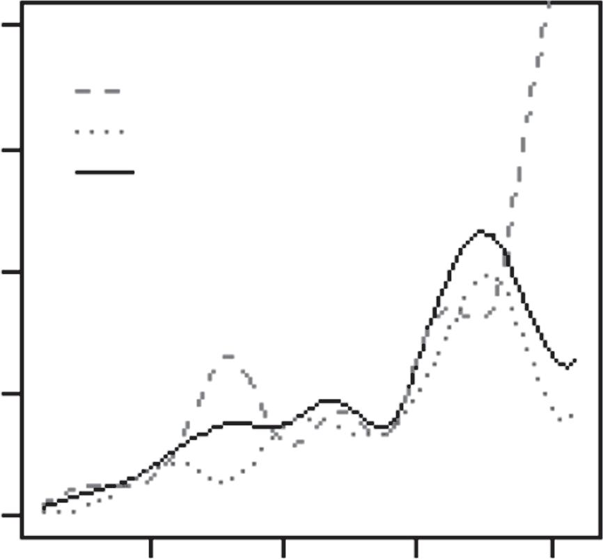
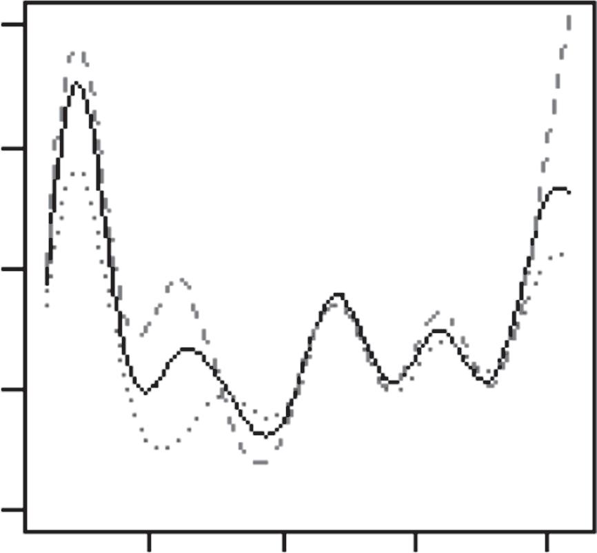
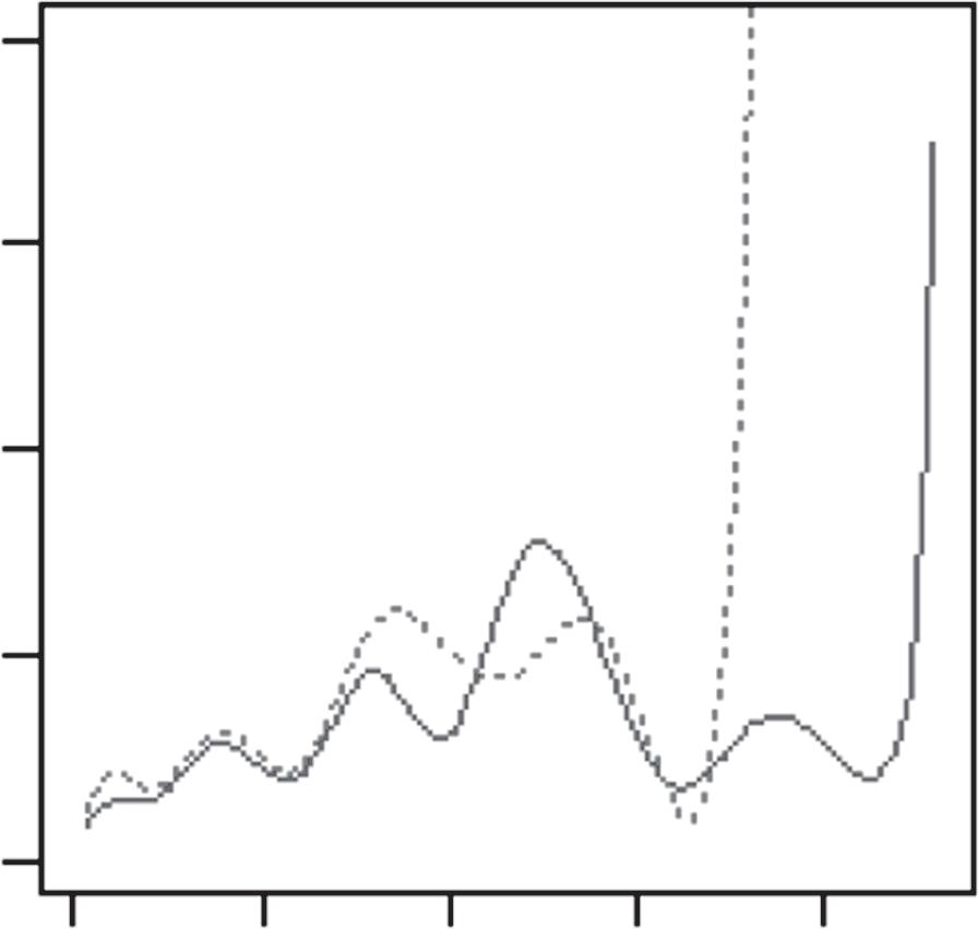
Byfollowingthemovementoftheballinthismannerwith K=3,wefound thatboththeBostonCelticsandtheMiamiHeatplayedwithessentiallythe samethreegroupsofplayers:(i)pointguards;(ii)superstars(RayAllenand PaulPiercefortheCeltics,DwyaneWadeandLeBronJamesfortheHeat); and(iii)others.However,theirrespectiveratefunctions,λ1(t),λ2(t),andλ3(t), showedthatthetwoteamsplayedtheirgamesverydifferently(Figure1.1).For theMiamiHeat,the“bump”between t ∈ (5,10) intheir λ1(t) wasbecause theirpointguardsusuallypassedtheballtoLeBronJamesandDwyaneWade andreliedonthetwoofthemtoorganizetheoffense;whereas,fortheBoston Celtics,therewasactuallya“dip”intheir λ1(t) between t ∈ (5,10).Thiswas becausetheirpointguards—mostnotably,RajonRondo—typicallyheldonto theballandorganizedtheoffensethemselves.

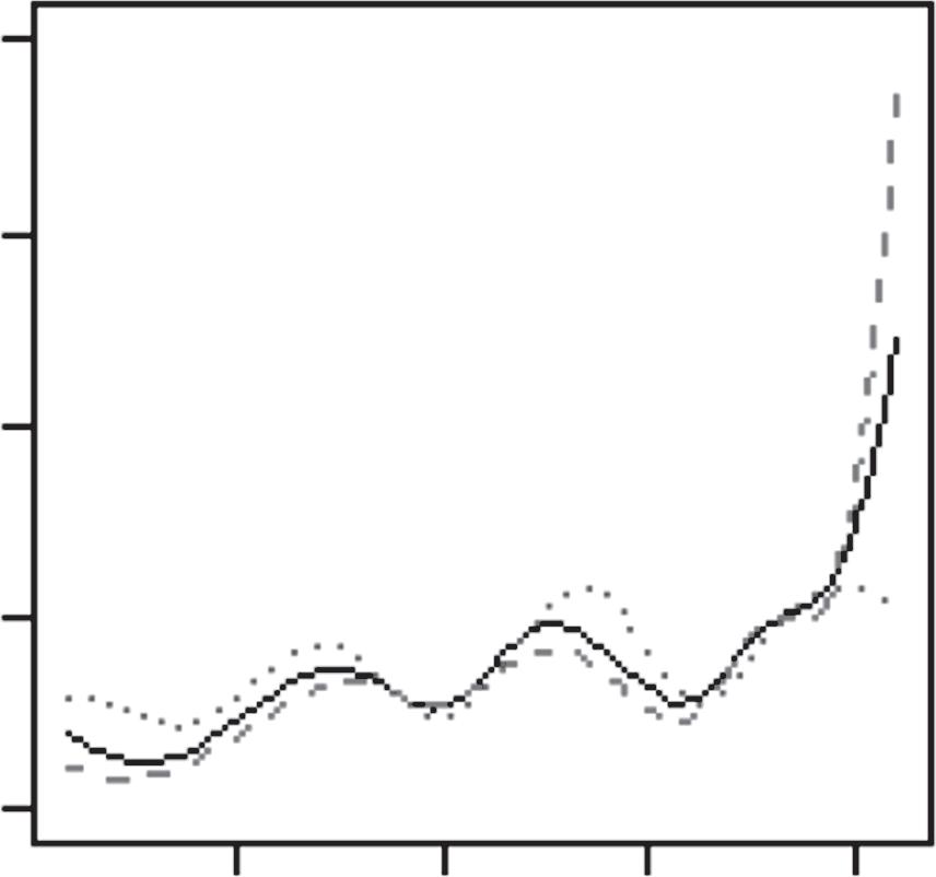
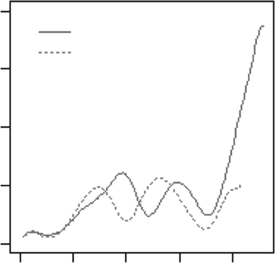
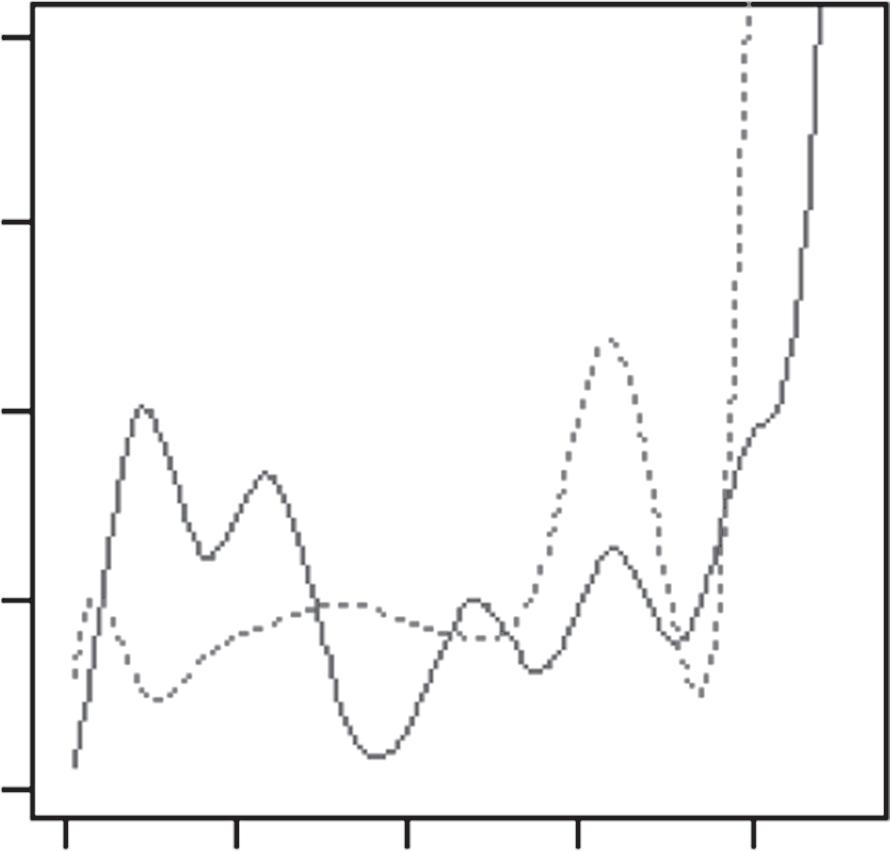
Inasimilarfashion,wefoundthat,duringthe2015finals,theGolden StateWarriorsplayedGame5verydifferentlyfromhowtheyhadplayed Game2.Inparticular,theirλ3(t)changeddramaticallybetweenthetwogames (Figure 1.2).Thiswasalmostcertainlybecausetheplayersinthisthirdgroup hadchangedaswell(Table 1.5).Morespecifically,twooftheirplayers,Andre IguodalaandDraymondGreen,appearedtohaveplayedverydifferentroles inthosetwogames.Readerswhoarefamiliarwiththe2014–2015seasonof theNBAwillbeabletorecallthat,duringthe2015finals,theGoldenState WarriorslostbothGames2and3,atwhichpointtheirheadcoach,SteveKerr,

Figure1.1 EstimatedratefunctionsforthreegroupsofplayersontheMiami HeatandthoseontheBostonCeltics,basedonGame1andGame5fromthe 2012NBAEasternConferencefinalsbetweenthetwoteams.

Source:ReprintedfromL.Xin,M.Zhu,H.Chipman(2017).“Acontinuous-timestochasticblock modelforbasketballnetworks”, AnnalsofAppliedStatistics, 11:553–597.Copyright2017,with permissionfromtheInstituteofMathematicalStatistics.

Figure1.2 EstimatedratefunctionsforthreegroupsofplayersontheGolden StateWarriors,basedonGame2andGame5,respectively,fromtheir2015NBA finalsagainsttheClevelandCavaliers.

Table1.5 GroupingofplayersontheGoldenStateWarriors, basedonGame2andGame5,respectively,fromtheir2015NBA finalsagainsttheClevelandCavaliers

AndreIguodala Centers DraymondGreen

SGs AndreIguodala SF+PFDraymondGreen

PG=pointguard(StephenCurry+ShaunLivingston);

SG=shootingguard(KlayThompson+LeandroBarbosa);

SF=shootingforward(HarrisonBarnes); PF=powerforward(DavidLee).

Theon-courtpositionsforIguodalaandGreenareSFandPF.Theanalysisgroups playersbyhowthey actually played,ratherthanhowtheywere supposed tohave played,eachgame.

Source:authors.

famouslydecidedtochangetheirregularline-uptoasmallline-upbystopping toplaycenters.Thiswasanunconventionalstrategy,butitsuccessfullyturned theseriesaround,andtheWarriorswentontowinthechampionshipbywinningthreeconsecutivegames.Ourmodelwasapparentlycapableofdetecting

thischangebysimplyfollowingthemovementoftheball,withoutexplicitly beingawareofthispieceofinformationwhatsoever.

Onereasonwhywesingledouttheseparticulargamestoanalyzewas becauseLeBronJameshadplayedbothforthe2011–2012MiamiHeatandfor the2014–2015ClevelandCavaliersanditwasinterestingtoexaminehowhe playedwiththesetwodifferentteams.Bycreatingtwoseparateavatarsforhim andtreatingthemastwo“players”inthemodel,weanalyzedplayersonthese twoteamstogether,usingK=4.Thefourgroupsofplayersturnedouttobe:(i) pointguards;(ii)LeBronJamesofthe2011–2012MiamiHeat,DwyaneWade, andLeBronJamesofthe2014–2015ClevelandCavaliers;(iii)otherperimeter players;and(iv)powerforwardsandcenters.Here,weseethatLeBronJames isaveryspecialplayerindeed.WiththeexceptionofDwyaneWade,nobody elseonthesetwoteamsplayedlikehim.Byandlarge,hebelongedtoagroupof hisown.Infact,somelong-timeobservershavesuggestedthathisdistinctive playingstylealmostcalledforthecreationofanewon-courtposition:point forward.Ouranalysiscertainlycorroboratessuchapointofview. □

ThroughExamples 1.1–1.3 above,wecanalreadygetaclearglimpseofthe statisticalbackboneofdatascience:first,aprobabilitymodelispostulatedto describethedata-generatingprocess;next,theunobservablequantitiesinthe modelareestimatedfromtheobservableones;finally,theestimatedmodelis usedtorevealpatterns,gaininsights,andmakepredictions.Itiscommonfor studentstothinkthatalgorithmsarethecoreofdatascience,but,inthestatisticalapproach,theirroleisstrictlysecondary—theyare“merely”incurredby theneedtoestimatetheunobservablequantitiesinaprobabilitymodelfrom theobservableones.

Appendix1.A Forbraveeyesonly

TobetterunderstandtheexpressioninsidethecurlybracketsinEquation(1.2), imaginepartitioningthetimeperiod (t0,t∞) intomanytinyintervalssuch that,oneachinterval,thereiseitherjustoneoccurrenceoftheunderlying event(here,acommunicationbetween i and j)ornooccurrenceatall.Then, omittingthesubscripts,“zizj”and“ij”,respectively,fromρziz j andtijh,theprobabilitythatthereareoccurrencesatcertaintimepointsandnoneelsewhereis, inthesamespiritasmodel(1.1),proportionalto

wherethenotations“th ∈ yes”and“th ∈ no”meanallthosetimeintervals withandwithoutanoccurrence,respectively.But

whichiswhythefirstproductinEquation(1.3)becomes [e –∫ρ

u)du] in Equation(1.2).[Note:Thetwoconvergencesigns“⟶”abovearebothresults ofpartitioningthetimeaxisintoinfinitelymanytinyintervals.Thefirst(†)is because,onallintervalsth ∈ nowithnooccurrence,theratefunctionρ(th)must berelativelysmall,and log(1– u) ≈ –u for u ≈ 0;morespecifically,theline tangentto log(1–u) atu =0 is –u.Thesecond(‡)isbasedontheRiemannsum approximationofintegrals.]

BuildingVocabulary

Thischapterbuildsthebasicvocabularyforspeakingthelanguageofprobability,fromsomefundamentallawstothenotionofrandomvariablesand theirdistributions.Forsomestudents,thiswilljustbeaquickreview,butit isalsopossibleforthosewhohaven’tlearnedanyofthesetoreadthischapter andlearnenoughinordertocontinuewiththerestofthebook.

2.1 Probability

Inprobability,the samplespace S isthecollectionofallpossibleoutcomes whenanexperimentisconducted,andanevent A ⊂ Sisasubsetofthesample space.Then,theprobabilityofanevent A issimply ℙ(A)=|A|/|S|,where“|·|” denotesthesizeoftheset.

Example2.1.Forexample,ifweindependentlytosstworegular,unloaded, six-faceddice,thesamplespaceissimply S ={(1,1), (1,2), (1,3), (1,4), (1,5), (1,6), (2,1), (2,2), (2,3), (2,4), (2,5), (2,6), (3,1), (3,2), (3,3), (3,4), (3,5), (3,6), (4,1), (4,2), (4,3), (4,4), (4,5), (4,6), (5,1), (5,2), (5,3), (5,4), (5,5), (5,6), (6,1), (6,2), (6,3), (6,4), (6,5), (6,6)},

acollectionofallpossibleoutcomes,andtheevent A ={obtainasumof 10} issimplythesubset

A ={(4,6),(5,5),(6,4)} ⊂ S, so ℙ(A)=3/36 Likewise,theevent B ={thetwodicedonotshowidenticalresult} issimplythesubset

B = S\{(1,1),(2,2),...,(6,6)}, EssentialStatisticsforDataScience.MuZhu,OxfordUniversityPress.©MuZhu(2023). DOI:10.1093/oso/9780192867735.003.0002

where“A\B”denotessetsubtraction,thatis, A\B ≡ A ∩ Bc,so ℙ(B)=(36–6) /36=30/36. □

Thisbasicnotionofprobabilityhereexplainswhythestudyofprobabilityalmostalwaysstartswithsomeelementsofcombinatorics,thatis,howto count.Indeed,countingcorrectlycanbequitetrickysometimes,butitisnota topicthatwewillcovermuchinthisbook.Somerudimentaryexperiencewith basiccombinatorics,say,atahigh-schoollevel,willbemorethanenoughto readthisbook.

2.1.1 Basicrules

Westatesome“obvious”rules.For A,B ⊂ S,

(a) ℙ(S)=1, ℙ(ϕ)=0, 0≤ ℙ(A)≤1,where ϕ denotestheemptyset;

(b) ℙ(Ac)=1– ℙ(A),where Ac denotesthecomplementof A ortheevent {not A};

Rules(a)–(b)abovehardlyrequireanyexplanation,whereasrule(c)canbe seenbysimplydrawinga Venndiagram (Figure 2.1).

Exercise2.1.UsetheVenndiagramtoconvinceyourselfofthefollowing identities:

Theseareknownas DeMorgan’slaws.

Figure2.1 AVenndiagram. Source:authors.

2.2 Conditionalprobability

Averyimportantconceptisthenotionofconditionalprobability.

Definition1 (Conditionalprobability). Thequantity

ℙ(A|B)= ℙ(A ∩ B) ℙ(B)

iscalledtheconditionalprobabilityof A given B. □

Itisusefultodevelopastrongintuitivefeelforwhytheconditionalprobabilityissodefined.Ifweknow B hasoccurred,thenthisadditionalpieceof informationeffectivelychangesoursamplespaceto B becauseanythingoutsidetheset B isnowirrelevant.Withinthisnew,effectivesamplespace,onlya subsetof A stillremains—specifically,thepartalsosharedby B,thatis, A ∩ B Thus,theeffectofknowing“B hasoccurred”istorestrictthesamplespace S to B andtheset A to A ∩ B.

Example2.2.RecallExample 2.1 insection 2.1.Whathappenstotheprobabilityof A ifweknow B hasoccurred?¹ If B hasoccurred,iteffectivelychanges oursamplespaceto { (1,2), (1,3), (1,4), (1,5), (1,6), (2,1), (2,3), (2,4), (2,5), (2,6), (3,1), (3,2), (3,4), (3,5), (3,6), (4,1), (4,2), (4,3), (4,5), (4,6), (5,1), (5,2), (5,3), (5,4), (5,6), (6,1), (6,2), (6,3), (6,4), (6,5), }

becausetheelements (1,1),(2,2), ,(6,6) arenowimpossible.Inthisnew, effectivesamplespace(ofsize 30),howmanywaysaretherefor A (asum of 10)tooccur?Clearly,theansweristwo—(4,6)and(6,4).Sotheconditional probabilityof A,given B,is ℙ(A|B)=2/30. □

2.2.1 Independence

Intuitively,itmakessensetosaythattwoevents(e.g. A and B)are independent ifknowingonehasoccurredturnsouttohavenoimpactonhowlikelythe

¹ ThisexamplehasbeenadaptedfromtheclassictextbySheldonRoss[5].

otherwilloccur,thatis,if

(A|B)= ℙ(A).

ByEquation(2.1),thisisthesameas

(A ∩ B)= ℙ(A)ℙ(B).

That’swhyweareoftentoldthat“independencemeansfactorization”. AtrivialrearrangementofEquation(2.1)gives

(A ∩ B)= ℙ(A|B)ℙ(B) or ℙ(B|A)ℙ(A).

Theseareactuallyhow jointprobabilities (of A and B)mustbecomputedin generalwhenindependence(between A and B)cannotbeassumed.

Exercise2.2.EllenandFrankhaveameeting.Let

E ={Ellenislate} and F ={Frankislate}.

Suppose ℙ(E)=0.1and ℙ(F)=0.3.Whatistheprobabilitythattheycanmeet ontime:

(a) if E isindependentof F;

(b) if ℙ(F|E)=0.5> ℙ(F);

Inwhichcase—(a),(b),or(c)—istheprobability(ofthemmeetingontime) thehighest?Doesthismakeintuitivesense? □

Remark2.1.Thistoyproblemneverthelessillustratessomethingmuch deeper.Often,therearemultipleriskfactorsaffectingtheprobabilityofa desiredoutcome,andtheanswercanbeverydifferentwhethertheserisk factorsareoperating(i)independentlyofeachother,(ii)inthe“samedirection”,or(iii)in“oppositedirections”.Toalargeextent,misjudginghow differentriskfactorsaffectedeachotherwaswhythe2008financialcrisis shockedmanyseasonedinvestors. □

2.2.2 Lawoftotalprobability

Ifthesamplespace S ispartitionedintodisjointpieces B1,B2,...,Bn suchthat S = n ⋃ i=1 Bi and Bi ∩ Bj = ϕ for i ≠ j, then,ascanbeeasilyseenfromFigure 2.2,

wherethestepmarkedby“⋆”isduetoEquation(2.4).Equation(2.5)isknown asthe lawoftotalprobability.

Eventhoughthislawisprettyeasytoderive,itsimplicationsarequite profound.Itgivesusaverypowerfulstrategyforcomputingprobabilities— namely,iftheprobabilityofsomething(e.g. A)ishardtocompute,lookfor extrainformation(e.g. B1,B2,...,Bn)sothattheconditionalprobabilities, givenvariousextrainformation, ℙ(A|B1), ℙ(A|B2),..., ℙ(A|Bn),maybeeasier tocompute;then,pieceeverythingtogether.

Whileallofthismaystillsoundratherstraightforward,truemasteryof thistechniqueisnoteasytoacquirewithoutconsiderableexperience,asthe followingexamplewilldemonstrate.

Example2.3.Adeckofrandomlyshuffledcardscontains n “regular”cards plusonejoker.(Forconvenience,wewillrefertosuchadeckas Dn.)YouandI taketurnstodrawfromthisdeck(withoutreplacement).Theonewhodraws

Figure2.2 Illustratingthelawoftotalprobability. Source:authors.

thejokerfirstwillwinacashprize.Yougofirst.What’stheprobabilityyouwill win?

Atfirstglance,thesituationhereseemsrathercomplex.Onsecondthoughts, werealizethatthesituationiseasierwhen n isrelativelysmall.Infact,the extremecaseof n =1 istrivial.Theanswerissimply 1/2 ifyoudrawfrom D1—withequalchance,eitheryoudrawthejokerandwinimmediatelyoryou drawtheonlyothercard,inwhichcase,Iwilldrawthejokernextandyouare suretolose.

Whathappenswhenyoudrawfrom D2 instead?Let W ={youwin}.

Whatextrainformationcanwelookfortohelpuspinpointtheprobability of W?Whatabouttheoutcomeofyourveryfirstdraw?Let

J ={yourfirstdrawisthejoker}.

Then,bythelawoftotalprobability,

(W)= ℙ(W|J)ℙ(J)+ ℙ(W|Jc)ℙ(Jc). (2.6)

Clearly,ifyourfirstdrawisalreadythejoker,thenyouwinimmediately;so ℙ(W|J)=1.Ifyourfirstdrawisnotthejoker,thenit’smyturntodraw.ButI nowdrawfromareduceddeck, D1,sinceyouhavealreadydrawna“regular” card.Aswehavealreadyarguedabove,mychanceofwinningwhiledrawing from D1 is 1/2,soyourchanceofwinningatthispointis 1–1/2=1/2.Thus, Equation(2.6)becomes

Itisnothardtoseenowthatthisreasoningprocesscanbecarriedforward inductively—ifyoudon’tdrawthejokerimmediatelyfrom Dn,thenit’smy turntodrawfrom Dn–1.Let

pn = ℙ(youwinwith Dn).

Then,theinductivestepis pn =(1)( 1 n +1) +(1– pn–1)(

), with p1 =1/2 beingthebaselinecase. □

ℙ