*Formu lt iples(mi l l i,mega,etc),seet heResou rcesec t ion
Conversion fac tors
θ/°C = T/K273.15*
1eV1.602177 × 1019J
96.485kJmol1
8065.5cm1 1cal4.184*J
1atm101.325*kPa
760*Torr 1cm11.9864 × 1023J
1D3.33564 × 1030Cm1Å1010m*
*E xac tva lue
Mathematical relations
π = 3.14159265359…e = 2.71828182846…
Logarithms and exponentials
ln x + ln y + … = ln xy…ln x ln y = ln(x/y)
a ln x = ln xa ln x = (ln10)log x = (2302585)log x
exeyez = ex+y+z+ ex/ey = ex y
Series expansions
(ex)a = eax e±ix = cos x ± isin x x x x e12 !3! x 23 = + + + + x x x x ln(1)23 23 + = + x x x 1 112 + = + x x x 1 112 = + + + x x x x sin3!5 ! 35 = + = + x x x cos12!4 ! 24
Derivatives; for Integrals, see the Resource section
d(f + g) = df + dg d(fg) = f dg + g df f g g f f g gd1dd 2 = f t f g g t f f g t d d d d ddfor(()) = = / y x x y 1 z z
y x x z z y 1 z y x
= x x nx d d n n 1 = x a de de ax ax = ax x x dln() d 1 =
f g x y x h x y y g y h x d(,)d(,)disexactif x y = +
Greek alphabet *
Α, α alpha Ι, ι iota Ρ, ρ rho
Β, β beta Κ, κ kappa Σ, σ sigma
Γ, γ gamma Λ, λ lambda Τ, τ tau
Δ, δ delta Μ, μ mu ϒ, υ upsilon
Ε, ε epsilon Ν, ν nu Φ, ϕ phi
Ζ, ζ zeta Ξ, ξ xi Χ, χ chi
Η, η etaΟ,οomicron Ψ, ψ psi
Θ, θ theta Π, π pi Ω, ω omega
*Obl iqueversions(α, β,…)a reusedtodenotephysica l
obser vables.
3 7 Rb 3 8 Sr
Numerical values of molar mass es in grams per mole (atomic weights) are quoted to the number of signi cant gures typical of most naturally occurring samples.
FUNDAMENTAL CONSTANTS
Exact value. For current values of the constants, see the National Institute of Standards and Technology (NIST) website.
Atkins’ PHYSICAL CHEMISTRY
Twelfth edition
Peter Atkins
Fellow of Lincoln College, University of Oxford, Oxford, UK
Julio de Paula
Professor of Chemistry, Lewis & Clark College, Portland, Oregon, USA
James Keeler
Associate Professor of Chemistry, University of Cambridge, and Walters Fellow in Chemistry at Selwyn College, Cambridge, UK
Great Clarendon Street, Oxford, OX2 6DP, United Kingdom
All rights reserved. No part of this publication may be reproduced, stored in a retrieval system, or transmitted, in any form or by any means, without the prior permission in writing of Oxford University Press, or as expressly permitted by law, by licence or under terms agreed with the appropriate reprographics rights organization. Enquiries concerning reproduction outside the scope of the above should be sent to the Rights Department, Oxford University Press, at the address above
You must not circulate this work in any other form and you must impose this same condition on any acquirer
Published in the United States of America by Oxford University Press 198 Madison Avenue, New York, NY 10016, United States of America
British Library Cataloguing in Publication Data Data available
Library of Congress Control Number: 2022935397
ISBN 978–0–19–884781–6
Printed in the UK by Bell & Bain Ltd., Glasgow
Links to third party websites are provided by Oxford in good faith and for information only. Oxford disclaims any responsibility for the materials contained in any third party website referenced in this work.
PREFACE
Our Physical Chemistry is continuously evolving in response to users’ comments, our own imagination, and technical innovation. The text is mature, but it has been given a new vibrancy: it has become dynamic by the creation of an e-book version with the pedagogical features that you would expect. They include the ability to summon up living graphs, get mathematical assistance in an awkward derivation, find solutions to exercises, get feedback on a multiple-choice quiz, and have easy access to data and more detailed information about a variety of subjects. These innovations are not there simply because it is now possible to implement them: they are there to help students at every stage of their course.
The flexible, popular, and less daunting arrangement of the text into readily selectable and digestible Topics grouped together into conceptually related Focuses has been retained. There have been various modifications of emphasis to match the evolving subject and to clarify arguments either in the light of readers’ comments or as a result of discussion among ourselves. We learn as we revise, and pass on that learning to our readers. Our own teaching experience ceaselessly reminds us that mathematics is the most fearsome part of physical chemistry, and we likewise ceaselessly wrestle with finding ways to overcome that fear. First, there is encouragement to use mathematics, for it is the language of much of physical chemistry. The How is that done? sections are designed to show that if you want to make progress with a concept, typically making it precise and quantitative, then you have to deploy mathematics. Mathematics opens doors to progress. Then there is the fine-grained help with the manipulation of equations, with their detailed annotations to indicate the steps being taken.
Behind all that are The chemist’s toolkits, which provide brief reminders of the underlying mathematical techniques. There is more behind them, for the collections of Toolkits available via the e-book take their content further and provide illustrations of how the material is used.
The text covers a very wide area and we have sought to add another dimension: depth. Material that we judge too detailed for the text itself but which provides this depth of treatment, or simply adds material of interest springing form the introductory material in the text, can now be found in enhanced A deeper look sections available via the e-book. These sections are there for students and instructors who wish to extend their knowledge and see the details of more advanced calculations.
The main text retains Examples (where we guide the reader through the process of answering a question) and Brief illustrations (which simply indicate the result of using an equation, giving a sense of how it and its units are used). In this edition a few Exercises are provided at the end of each major section in a Topic along with, in the e-book, a selection of multiple-choice questions. These questions give the student the opportunity to check their understanding, and, in the case of the e-book, receive immediate feedback on their answers. Straightforward Exercises and more demanding Problems appear at the end of each Focus, as in previous editions.
The text is living and evolving. As such, it depends very much on input from users throughout the world. We welcome your advice and comments.
USING THE BOOK
TO THE STUDENT
The twelfth edition of Atkins’ Physical Chemistry has been developed in collaboration with current students of physical chemistry in order to meet your needs better than ever before. Our student reviewers have helped us to revise our writing style to retain clarity but match the way you read. We have also introduced a new opening section, Energy: A first look, which summarizes some key concepts that are used throughout the text and are best kept in mind right from the beginning. They are all revisited in greater detail later. The new edition also brings with it a hugely expanded range of digital resources, including living graphs, where you can explore the consequences of changing parameters, video interviews with practising scientists, video tutorials that help to bring key equations to life in each Focus, and a suite of self-check questions. These features are provided as part of an enhanced e-book, which is accessible by using the access code included in the book. You will find that the e-book offers a rich, dynamic learning experience. The digital enhancements have been crafted to help your study and assess how well you have understood the material. For instance, it provides assessment materials that give you regular opportunities to test your understanding.
Innovative structure
Short, selectable Topics are grouped into overarching Focus sections. The former make the subject accessible; the latter provides its intellectual integrity. Each Topic opens with the questions that are commonly asked: why is this material important?, what should you look out for as a key idea?, and what do you need to know already?
Resource section
AVAILABLE IN THE E-BOOK
‘Impact on…’ sections
Impact on sections show how physical chemistry is applied in a variety of modern contexts. They showcase physical chemistry as an evolving subject.
Go to this location in the accompanying e-book to view a list of Impacts.
‘A deeper look’ sections
These sections take some of the material in the text further and are there if you want to extend your knowledge and see the details of some of the more advanced derivations.
Go to this location in the accompanying e-book to view a list of Deeper Looks.
Group theory tables
A link to comprehensive group theory tables can be found at the end of the accompanying e-book.
The chemist’s toolkits
The chemist’s toolkits are reminders of the key mathematical, physical, and chemical concepts that you need to understand in order to follow the text.
For a consolidated and enhanced collection of the toolkits found throughout the text, go to this location in the accompanying e-book.
TOPIC 2A Internal energy
RESOURCE SECTION
An isolated system can exchange neither energy nor matter with its surroundings.
2A.1 Work, heat, and energy
Although thermodynamics deals with the properties of bulk systems, it is enriched by understanding the molecular origins of these properties. What follows are descriptions of work, heat, and energy from both points of view.
2A.1(a) Definitions
The Resource section at the end of the book includes a brief review of two mathematical tools that are used throughout the text: differentiation and integration, including a table of the integrals that are encountered in the text. There is a review of units, and how to use them, an extensive compilation of tables of physical and chemical data, and a set of character tables. Short extracts of most of these tables appear in the Topics themselves: they are there to give you an idea of the typical values of the physical quantities mentioned in the text.
In thermodynamics, the universe is divided into two parts: the system and its surroundings. The system is the part of the world of interest. It may be a reaction vessel, an engine, an electrochemical cell, a biological cell, and so on. The surroundings comprise the region outside the system. Measurements are made in the surroundings. The type of system depends on the characteristics of the boundary that divides it from the surroundings (Fig. 2A.1): An open system has a boundary through which matter can be transferred.
The fundamental physical property in thermodynamics is work: work is done in order to achieve motion against an opposing force (Energy: A first look 2a). A simple example is the process of raising a weight against the pull of gravity. A process does work if in principle it can be harnessed to raise a weight somewhere in the surroundings. An example is the expansion of a gas that pushes out a piston: the motion of the piston can in principle be used to raise a weight. Another example is a chemical reaction in a battery: the reaction generates an electric current that can drive a motor and be used to raise a weight.
The energy of a system is its capacity to do work (Energy: A first look 2b). When work is done on an otherwise isolated system (for instance, by compressing a gas with a piston or winding a spring), the capacity of the system to do work is increased. That is, the energy of the system is increased. When the system does work (when the piston moves out or the spring unwinds), it can do less work than before. That is, its energy is decreased. When a gas is compressed by a piston, work is done on the system and its energy is increased. When that gas is allowed to expand again the piston moves out, work is done by the system, and the energy of the system is decreased.
It is very important to note that when the energy of the system increases that of the surroundings decreases by exactly the same amount, and vice versa. Thus, the weight raised when the system does work has more energy than before the expansion, because a raised weight can do more work than a lowered one. The weight lowered when work is done on the system has less
TOPIC 2B Enthalpy
Checklist of concepts
A checklist of key concepts is provided at the end of each Topic, so that you can tick off the ones you have mastered.
➤ Why do you need to know this material?
The concept of enthalpy is central to many thermodynamic discussions about processes, such as physical transformations and chemical reactions taking place under conditions of constant pressure.
Physical chemistry: people and perspectives
➤ What is the key idea?
A change in enthalpy is equal to the energy transferred as heat at constant pressure.
Leading figures in a varity of fields share their unique and varied experiences and careers, and talk about the challenges they faced and their achievements to give you a sense of where the study of physical chemistry can lead.
➤ What do you need to know already?
This Topic makes use of the discussion of internal energy (Topic 2A) and draws on some aspects of perfect gases (Topic 1A).
PRESENTING THE MATHEMATICS
How is that done?
The change in internal energy is not equal to the energy transferred as heat when the system is free to change its volume, such as when it is able to expand or contract under conditions of constant pressure. Under these circumstances some of the energy supplied as heat to the system is returned to the surroundings as expansion work (Fig. 2B.1), so dU is less than dq. In this case the energy supplied as heat at constant pressure is equal to the change in another thermodynamic property of the system, the ‘enthalpy’.
You need to understand how an equation is derived from reasonable assumptions and the details of the steps involved. This is one role for the How is that done? sections. Each one leads from an issue that arises in the text, develops the necessary equations, and arrives at a conclusion. These sections maintain the separation of the equation and its derivation so that you can find them easily for review, but at the same time emphasize that mathematics is an essential feature of physical chemistry.
The chemist’s toolkits
This relation provides a simple way of measuring the heat capacity of a sample. A measured quantity of energy is transferred
Checklist of concepts
2B.1 The definition of enthalpy
The enthalpy, H, is defined as
☐ 1. Work is the process of achieving motion against an opposing force.
☐ 2. Energy is the capacity to do work.
H UpV
☐ 3. Heat is the process of transferring energy as a result of a temperature difference.
Enthalpy [definition] (2B.1)
☐ 4. An exothermic process is a process that releases energy
where p is the pressure of the system and V is its volume. Because U, p, and V are all state functions, the enthalpy is a state function too. As is true of any state function, the change in enthalpy, ΔH, between any pair of initial and final states is independent of the path between them.
☐ process is a process in which energy is
2B.1(a) Enthalpy change and heat transfer
☐ In molecular terms, work is the transfer of energy that makes use of organized motion of atoms in the surroundings and heat is the transfer of energy that makes
☐ , the total energy of a system, is a state
Probability = |ψ|2dx
An important consequence of the definition of enthalpy in eqn 2B.1 is that it can be shown that the change in enthalpy is equal to the energy supplied as heat under conditions of constant pressure.
How is that done? 2B.1 Deriving the relation between enthalpy change and heat transfer at constant pressure
In a typical thermodynamic derivation, as here, a common way to proceed is to introduce successive definitions of the quantities of interest and then apply the appropriate constraints.
Step 1 Write an expression for H + dH in terms of the definition of H
Figure 7B.1 The wavefunction ψ is a probability amplitude in the sense that its square modulus (ψ ⋆ ψ or |ψ|2) is a probability density. The probability of finding a particle in the region between x and x + dx is proportional to |ψ|2dx. Here, the probability density is represented by the density of shading in the superimposed band.
For a general infinitesimal change in the state of the system, U changes to U + dU, p changes to p + dp, and V changes to V + dV, so from the definition in eqn 2B.1, H changes by d H to
13A The Boltzmann distribution 545
The chemist’s toolkit 7B.1 Complex numbers
Figure 7B.2 dimensional particle in the proportional position.
The chemist’s toolkits are reminders of the key mathematical, physical, and chemical concepts that you need to understand in order to follow the text. Many of these Toolkits are relevant to more than one Topic, and you can view a compilation of them, with enhancements in the form of more information and brief illustrations, in this section of the accompanying e-book.
If, as a result of collisions, the system were to fluctuate between the configurations {N,0,0,…} and {N 2,2,0,…}, it would almost always be found in the second, more likely configuration, especially if N were large. In other words, a system free to switch between the two configurations would show properties characteristic almost exclusively of the second configuration.
Brief illustration 13A.1
Annotated equations and equation labels
The next step is to develop an expression for the number of ways that a general configuration {N0,N1,…} can be achieved. This number is called the weight of the configuration and denoted W
We have annotated many equations to help you follow how they are developed. An annotation can help you travel across the equals sign: it is a reminder of the substitution used, an approximation made, the terms that have been assumed constant, an integral used, and so on. An annotation can also be a reminder of the significance of an individual term in an expression. We sometimes collect into a small box a collection of numbers or symbols to show how they carry from one line to the next. Many of the equations are labelled to highlight their significance.
Figure 2B.1 When a system is subjected to constant pressure and is free to change its volume, some of the energy supplied as heat may escape back into the surroundings as work. In such a case, the change in internal energy is smaller than the energy supplied as heat.
How is that done? 13A.1
Evaluating the weight of a configuration
Consider the number of ways of distributing N balls into bins labelled 0, 1, 2 … such that there are N0 balls in bin 0, N1 in bin 1, and so on. The first ball can be selected in N different ways, the next ball in N 1 different ways from the balls remaining, and so on. Therefore, there are N(N 1) … 1 = N! ways of selecting the balls.
There are N0! different ways in which the balls could have been chosen to fill bin 0 (Fig. 13A.1). Similarly, there are N1! ways in which the balls in bin 1 could have been chosen, and so on. Therefore, the total number of distinguishable ways of
The last term is the product of two infinitesimally small quantities and can be neglected. Now recognize that U + pV = H on the right (boxed), so
For the configuration {1,0,3,5,10,1}, which has N = 20, the weight is calculated as (recall that 0! ≡ 1) W 20 1035101 93110 !8 !!!!!!
A complex number z has the form z = x + iy, where i1. The complex conjugate of a complex number z is z* = x iy Complex numbers combine together according to the following rules:
Addition and subtraction:
and hence
()()()() ab cd ac bd iii
dddd HU pV Vp
Multiplication:
It will turn out to be more convenient to deal with the natural logarithm of the weight, ln W , rather than with the weight itself:
Step 2 Introduce the definition of dU
()()()() ab cd ac bdbc ad iii
Because dU = d q + dw this expression becomes
Two special relations are:
ddddd d Hq wp VV p U
Modulus: ||()() zz zx y 122212 //
Euler’s relation: ei i cossin , which implies that ei1, cos() 1 2ee ii , and sin() 1 2ieeii .
ln(x/y) = ln x ln y ln xy = ln x + ln y ( NN NN n!!!012)
NN NN NN ln!ln!ln!ln!ln!ln! i i 012 =− ∑
One reason for introducing ln W is that it is easier to make approximations. In particular, the factorials can be simplified by using Stirling’s approximation1 ln!ln xx xx Stirling’sapproximation[ >> 1] x (13A.2)
Then the approximate expression for the weight is
Because |ψ|2dx is a (dimensionless) probability, |ψ|2 is the probability density, with the dimensions of 1/length (for a one-dimensional system). The wavefunction ψ itself is called the probability amplitude. For a particle free to move in three dimensions (for example, an electron near a nucleus in an atom), the wavefunction depends on the coordinates x, y, and z and is denoted ψ(r). In this case the Born interpretation is
The Born significance because |ψ direct significance function: only cant, and both may correspond region (Fig. tive regions because it structive interference A wavefunction
☐ 8. The internal raised.
☐ 9. The First lated system
☐ 10. Free expansion no work.
☐ 11. A reversible an infinitesimal
12. To achieve sure is system.
13. The energy equal to
14. Calorimetry
Figure 7B.3 physical significance: this wavefunction distribution the density
☐ 1. Energy transferred as heat at constant pressure is equal to the change in enthalpy of a system.
Enthalpy changes can be measured in an isobaric calorimeter.
Checklists of equations
A handy checklist at the end of each topic summarizes the most important equations and the conditions under which they apply. Don’t think, however, that you have to memorize every equation in these checklists: they are collected there for ready reference.
Video tutorials on key equations
Video tutorials to accompany each Focus dig deeper into some of the key equations used throughout that Focus, emphasizing the significance of an equation, and highlighting connections with material elsewhere in the book.
48 2 The First Law
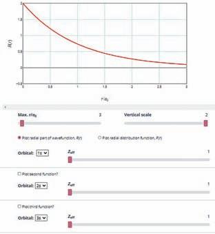
Living graphs
The educational value of many graphs can be heightened by seeing—in a very direct way—how relevant parameters, such as temperature or pressure, affect the plot. You can now interact with key graphs throughout the text in order to explore how they respond as the parameters are changed. These graphs are clearly flagged throughout the book, and you can find links to the dynamic versions in the corresponding location in the e-book.
Checklist of equations
Relation between heat capacities
Table 2B.1 Temperature variation of molar heat capacities, C(JK mol) = + + 11 2 p abTc T ,m // *
* More values are given in the Resource section
Atkins-Chap02_033-074.indd 49
SETTING UP AND SOLVING PROBLEMS
Brief illustrations
Figure 2B.3 The constant-pressure heat capacity at a particular temperature is the slope of the tangent to a curve of the enthalpy of a system plotted against temperature (at constant pressure). For gases, at a given temperature the slope of enthalpy versus temperature is steeper than that of internal energy versus temperature, and Cp,m is larger than CV,m Temperature, T
mass densities of the polymorphs are 2.71 g cm 3 (calcite) and 2.93 g cm 3 (aragonite).
A Brief illustration shows you how to use an equation or concept that has just been introduced in the text. It shows you how to use data and manipulate units correctly. It also helps you to become familiar with the magnitudes of quantities.
2B Enthalpy
The empirical parameters a, b, and c are independent of temperature. Their values are found by fitting this expression to experimental data on many substances, as shown in Table 2B.1. If eqn 2B.8 is used to calculate the change in enthalpy between two temperatures T1 and T2, integration by using Integral A.1 in the Resource section gives
Brief illustration 2B.2
is the heat capacity per mole of substance; it is an intensive property.
The heat capacity at constant pressure relates the change in enthalpy to a change in temperature. For infinitesimal changes of temperature, eqn 2B.5 implies that
Examples
Collect your thoughts The starting point for the calculation is the relation between the enthalpy of a substance and its internal energy (eqn 2B.1). You need to express the difference between the two quantities in terms of the pressure and the difference of their molar volumes. The latter can be calculated from their molar masses, M, and their mass densities, ρ, by using ρ = M/Vm
In the reaction 3 H2(g) + N2(g) → 2 NH3(g), 4 mol of gasphase molecules is replaced by 2 mol of gas-phase molecules, so Δn g = 2 mol. Therefore, at 298 K, when RT = 2 .5 kJ mol 1 , the molar enthalpy and molar internal energy changes taking place in the system are related by
HU RT mmkJ()mo . 25011
dd(atconstantpressure
HC T p = )
(2B.6a)
Worked Examples are more detailed illustrations of the application of the material, and typically require you to assemble and deploy several relevant concepts and equations. Everyone has a different way to approach solving a problem, and it changes with experience. To help in this process, we suggest how you should collect your thoughts and then proceed to a solution. All the worked Examples are accompanied by closely related self-tests to enable you to test your grasp of the material after working through our solution as set out in the Example
The solution The change in enthalpy when the transition occurs is
If the heat capacity is constant over the range of temperatures of interest, then for a measurable increase in temperature
T dd 1 2 1 2 21 () which can be summarized as
HC TC TC TT p T
HH H UpVU pV mmm mmmm aragonitecalcite aacc ()() {()()}{()()} } {()()}Up VV mmm ac
HC T p atconstantpressure ()
(2B.6b)
where a denotes aragonite and c calcite. It follows by substituting Vm = M/ρ that
Because a change in enthalpy can be equated to the energy supplied as heat at constant pressure, the practical form of this equation is
HU pM mm ac 11 ()()
q CT pp
Substitution of the data, using M = 100.09 g mol 1, gives
(2B.7)
This expression shows how to measure the constant-pressure heat capacity of a sample: a measured quantity of energy is supplied as heat under conditions of constant pressure (as in a sample exposed to the atmosphere and free to expand), and the temperature rise is monitored.
HU mm Pagm (.o 10)(.) 10100091 1 293 1 271 51 33
Example 2B.2 Evaluating an increase in enthalpy with temperature
Note that the difference is expressed in kilojoules, not joules as in Example 2B.1. The enthalpy change is more negative than the change in internal energy because, although energy escapes from the system as heat when the reaction occurs, the system contracts as the product is formed, so energy is restored to it as work from the surroundings.
What is the change in molar enthalpy of N2 when it is heated from 25 °C to 100 °C? Use the heat capacity information in Table 2B.1.
Collect your thoughts The heat capacity of N2 changes with temperature significantly in this range, so use eqn 2B.9.
Exercises
The solution Using a = 28.58
E2B.1 Calculate the value of ΔH m ΔUm for the reaction N2(g) + 3 H2(g) → 2 NH3(g) at 473 K.
is written as
E2B.2 When 0.100 mol of H2(g) is burnt in a flame calorimeter it is observed that the water bath in which the apparatus is immersed increases in temperature by 13.64 K. When 0.100 mol C4H10(g), butane, is burnt in the same apparatus the temperature rise is 6.03 K. The molar enthalpy of combustion of H2(g) is 285 kJ mol 1. Calculate the molar enthalpy of combustion of butane.
47
(2B.9)
Self-check questions
This edition introduces self-check questions throughout the text, which can be found at the end of most sections in the e-book. They test your comprehension of the concepts discussed in each section, and provide instant feedback to help you monitor your progress and reinforce your learning. Some of the questions are multiple choice; for them the ‘wrong’ answers are not simply random numbers but the result of errors that, in our experience, students often make. The feedback from the multiple choice questions not only explains the correct method, but also points out the mistakes that led to the incorrect answer. By working through the multiple-choice questions you will be well prepared to tackle more challenging exercises and problems.
Discussion questions
Discussion questions appear at the end of each Focus, and are organized by Topic. They are designed to encourage you to reflect on the material you have just read, to review the key concepts, and sometimes to think about its implications and limitations.
Exercises and problems
Exercises are provided throughout the main text and, along with Problems, at the end of every Focus. They are all organised by Topic. Exercises are designed as relatively straightforward numerical tests; the Problems are more challenging and typically involve constructing a more detailed answer. For this new edition, detailed solutions are provided in the e-book in the same location as they appear in print.
For the Examples and Problems at the end of each Focus detailed solutions to the odd-numbered questions are provided in the e-book; solutions to the even-numbered questions are available only to lecturers.
Integrated activities
At the end of every Focus you will find questions that span several Topics. They are designed to help you use your knowledge creatively in a variety of ways.
FOCUS 1 The properties of gases
To test your understanding of this material, work through the Exercises Additional exercises, Discussion questions, and Problems found throughout this Focus.
Selected solutions can be found at the end of this Focus in the e-book. Solutions to even-numbered questions are available online only to lecturers.
TOPIC 1A The perfect gas
Discussion questions
D1A.1 Explain how the perfect gas equation of state arises by combination of Boyle’s law, Charles’s law, and Avogadro’s principle.
Additional exercises
E1A.8 Express (i) 22.5 kPa in atmospheres and (ii) 770 Torr in pascals.
E1A.9 Could 25 g of argon gas in a vessel of volume 1.5 dm exert a pressure of 2.0 bar at 30 C if it behaved as a perfect gas? If not, what pressure would it exert?
E1A.10 A perfect gas undergoes isothermal expansion, which increases its volume by 2.20 dm . The final pressure and volume of the gas are 5.04 bar and 4.65 dm3 respectively. Calculate the original pressure of the gas in (i) bar, (ii) atm.
E1A.11 A perfect gas undergoes isothermal compression, which reduces its volume by 1.80 dm . The final pressure and volume of the gas are 1.97 bar and 2.14 dm3 respectively. Calculate the original pressure of the gas in (i) bar, (ii) torr.
E1A.12 A car tyre (an automobile tire) was inflated to a pressure of 24 lb in 2 (1.00 atm 14.7 lb in ) on a winter’s day when the temperature was 5 C. What pressure will be found, assuming no leaks have occurred and that the volume is constant, on a subsequent summer’s day when the temperature is 35 C? What complications should be taken into account in practice?
E1A.13 A sample of hydrogen gas was found to have a pressure of 125 kPa when the temperature was 23 °C. What can its pressure be expected to be when the temperature is 11 C?
E1A.14 A sample of 255 mg of neon occupies 3.00 dm at 122 K. Use the perfect gas law to calculate the pressure of the gas.
E1A.15 A homeowner uses 4.00 × 10 m 3 of natural gas in a year to heat a home. Assume that natural gas is all methane, CH4 and that methane is a perfect gas for the conditions of this problem, which are 1.00 atm and 20 C. What is the mass of gas used?
E1A.16 At 100 C and 16.0 kPa, the mass density of phosphorus vapour is 0.6388 kg m 3 What is the molecular formula of phosphorus under these conditions?
E1A.17 Calculate the mass of water vapour present in a room
D1A.2 Explain the term ‘partial pressure’ and explain why Dalton’s law is a limiting law.
FOCUS 4 Physical transformations of pure substances
Goodwin (J. Phys. Chem. Ref. Data 18, 1565 (1989)) presented expressions for two coexistence curves. The solid–liquid curve is given by p px x /bar /bar 1000 56011 727 (. .) where x T/T3 1 and the triple point pressure and temperature are p3 0.4362 μbar and T3 178.15 K. The liquid–vapour curve is given by ln( ). py yy y /bar / 10418211571599614015 5 0120 4 733 2 3 4 41()170 y where y T/T
Exercises
‘Impact’ sections
‘Impact ’ sections show you how physical chemistry is applied in a variety of modern contexts. They showcase physical chemistry as an evolving subject. These sections are listed at the beginning of the text, and are referred to at appropriate places elsewhere. You can find a compilation of ‘Impact ’ sections at the end of the e-book.
A deeper look
These sections take some of the material in the text further. Read them if you want to extend your knowledge and see the
TAKING YOUR LEARNING FURTHER TO THE INSTRUCTOR
We have designed the text to give you maximum flexibility in the selection and sequence of Topics, while the grouping of Topics into Focuses helps to maintain the unity of the subject. Additional resources are:
Figures and tables from the book
Lecturers can find the artwork and tables from the book in ready-to-download format. They may be used for lectures without charge (but not for commercial purposes without specific permission).
details of some of the more advanced derivations. They are listed at the beginning of the text and are referred to where they are relevant. You can find a compilation of Deeper Looks at the end of the e-book.
Group theory tables
If you need character tables, you can find them at the end of the Resource section.
Key equations
Supplied in Word format so you can download and edit them.
Solutions to exercises, problems, and integrated activities
For the discussion questions, examples, problems, and integrated activities detailed solutions to the even-numbered questions are available to lecturers online, so they can be set as homework or used as discussion points in class.
Lecturer resources are available only to registered adopters of the textbook. To register, simply visit www.oup.com/he/ pchem12e and follow the appropriate links.
ABOUT THE AUTHORS
Peter Atkins is a fellow of Lincoln College, Oxford, and emeritus professor of physical chemistry in the University of Oxford. He is the author of over seventy books for students and a general audience. His texts are market leaders around the globe. A frequent lecturer throughout the world, he has held visiting professorships in France, Israel, Japan, China, Russia, and New Zealand. He was the founding chairman of the Committee on Chemistry Education of the International Union of Pure and Applied Chemistry and was a member of IUPAC’s Physical and Biophysical Chemistry Division.
Julio de Paula is Professor of Chemistry at Lewis & Clark College. A native of Brazil, he received a B.A. degree in chemistry from Rutgers, The State University of New Jersey, and a Ph.D. in biophysical chemistry from Yale University. His research activities encompass the areas of molecular spectroscopy, photochemistry, and nanoscience. He has taught courses in general chemistry, physical chemistry, biochemistry, inorganic chemistry, instrumental analysis, environmental chemistry, and writing. Among his professional honours are a Christian and Mary Lindback Award for Distinguished Teaching, a Henry Dreyfus Teacher-Scholar Award, and a STAR Award from the Research Corporation for Science Advancement.
James Keeler is Associate Professor of Chemistry, University of Cambridge, and Walters Fellow in Chemistry at Selwyn College. He received his first degree and doctorate from the University of Oxford, specializing in nuclear magnetic resonance spectroscopy. He is presently Head of Department, and before that was Director of Teaching in the department and also Senior Tutor at Selwyn College.
A book as extensive as this could not have been written without significant input from many individuals. We would like to thank the hundreds of instructors and students who contributed to this and the previous eleven editions:
Scott Anderson, University of Utah
Milan Antonijevic, University of Greenwich
Elena Besley, University of Greenwich
Merete Bilde, Aarhus University
Matthew Blunt, University College London
Simon Bott, Swansea University
Klaus Braagaard Møller, Technical University of Denmark
Wesley Browne, University of Groningen
Sean Decatur, Kenyon College
Anthony Harriman, Newcastle University
Rigoberto Hernandez, Johns Hopkins University
J. Grant Hill, University of Sheffield
Kayla Keller, Kentucky Wesleyan College
Kathleen Knierim, University of Louisiana Lafayette
Tim Kowalczyk, Western Washington University
Kristin Dawn Krantzman, College of Charleston
Hai Lin, University of Colorado Denver
Mikko Linnolahti, University of Eastern Finland
Mike Lyons, Trinity College Dublin
Jason McAfee, University of North Texas
Joseph McDouall, University of Manchester
Hugo Meekes, Radboud University
Gareth Morris, University of Manchester
David Rowley, University College London
Nessima Salhi, Uppsala University
Andy S. Sardjan, University of Groningen
Trevor Sears, Stony Brook University
Gemma Shearman, Kingston University
John Slattery, University of York
Catherine Southern, DePaul University
Michael Staniforth, University of Warwick
Stefan Stoll, University of Washington
Mahamud Subir, Ball State University
Enrico Tapavicza, CSU Long Beach
Jeroen van Duifneveldt, University of Bristol
Darren Walsh, University of Nottingham
Graeme Watson, Trinity College Dublin
Darren L. Williams, Sam Houston State University
Elisabeth R. Young, Lehigh University
Our special thanks also go to the many student reviewers who helped to shape this twelfth edition:
Katherine Ailles, University of York
Mohammad Usman Ali, University of Manchester
Rosalind Baverstock, Durham University
Grace Butler, Trinity College Dublin
Kaylyn Cater, Cardiff University
Ruth Comerford, University College Dublin
Orlagh Fraser, University of Aberdeen
Dexin Gao, University College London
Suruthi Gnanenthiran, University of Bath
Milena Gonakova, University of the West of England Bristol
Joseph Ingle, University of Lincoln
Jeremy Lee, University of Durham
Luize Luse, Heriot-Watt University
Zoe Macpherson, University of Strathclyde
Sukhbir Mann, University College London
Declan Meehan, Trinity College Dublin
Eva Pogacar, Heriot-Watt University
Pawel Pokorski, Heriot-Watt University
Fintan Reid, University of Strathclyde
Gabrielle Rennie, University of Strathclyde
Annabel Savage, Manchester Metropolitan University
Sophie Shearlaw, University of Strathclyde
Yutong Shen, University College London
Saleh Soomro, University College London
Matthew Tully, Bangor University
Richard Vesely, University of Cambridge
Phoebe Williams, Nottingham Trent University
We would also like to thank Michael Clugston for proofreading the entire book, and Peter Bolgar, Haydn Lloyd, Aimee North, Vladimiras Oleinikovas, and Stephanie Smith who all worked alongside James Keeler in the writing of the solutions to the exercises and problems. The multiple-choice questions were developed in large part by Dr Stephanie Smith (Yusuf Hamied Department of Chemistry and Pembroke College, University of Cambridge). These questions and further exercises were integrated into the text by Chloe Balhatchet (Yusuf Hamied Department of Chemistry and Selwyn College, University of Cambridge), who also worked on the living graphs. The solutions to the exercises and problems are taken from the solutions manual for the eleventh edition prepared by Peter Bolgar, Haydn Lloyd, Aimee North, Vladimiras Oleinikovas, Stephanie Smith, and James Keeler, with additional contributions from Chloe Balhatchet.
Last, but by no means least, we acknowledge our two commissioning editors, Jonathan Crowe of Oxford University Press and Jason Noe of OUP USA, and their teams for their assistance, advice, encouragement, and patience. We owe special thanks to Katy Underhill, Maria Bajo Gutiérrez, and Keith Faivre from OUP, who skillfully shepherded this complex project to completion.
of condensed phases with
of the
TOPIC
TOPIC
7B.1
TOPIC
9B.1
FOCUS 11 Molecular spectroscopy 427
11A.1
TOPIC 11B Rotational spectroscopy
TOPIC
12C Pulse techniques in NMR 521
12C.1 The magnetization vector 521
(a) The effect of the radiofrequency field 522
(b) Time- and frequency-domain signals 523
12C.2 Spin relaxation 525
(a) The mechanism of relaxation 525
(b) The measurement of T1 and T 2 526
12C.3 Spin decoupling 527
12C.4 The nuclear Overhauser effect 528
Checklist of concepts 530
Checklist of equations 530
TOPIC 12D Electron paramagnetic resonance 531
12D.1 The g -value 531
12D.2 Hyperfine structure 532
(a) The effects of nuclear spin 532
12D.3 The McConnell equation 533
(a) The origin of the hyperfine interaction 534
Checklist of concepts 535
Checklist of equations 535
FOCUS 13 Statistical thermodynamics 543
TOPIC 13A The Boltzmann distribution 544
13A.1 Configurations and weights 544
(a) Instantaneous configurations 544
(b) The most probable distribution 545
13A.2 The relative populations of states 548
Checklist of concepts 549
Checklist of equations 549
TOPIC 13B Molecular partition functions 550
13B.1 The significance of the partition function 550
13B.2 Contributions to the partition function 552
(a) The translational contribution 552
(b) The rotational contribution 554
(c) The vibrational contribution 558
(d) The electronic contribution 559
Checklist of concepts 560
Checklist of equations 560
TOPIC 13C Molecular energies 561
13C.1 The basic equations 561
13C.2 Contributions of the fundamental modes of motion 562
(a) The translational contribution 562
(b) The rotational contribution 562
(c) The vibrational contribution 563
(d) The electronic contribution 564
(e) The spin contribution 565
Checklist of concepts 565
Checklist of equations 566
TOPIC 13D The canonical ensemble 567
13D.1 The concept of ensemble 567
(a) Dominating configurations
(b) Fluctuations from the most probable distribution 568
13D.2 The mean energy of a system 569
13D.3 Independent molecules revisited 569
13D.4 The variation of the energy with volume
TOPIC 13E The internal energy and the entropy
13E.1 The internal energy
(a) The calculation of internal energy
(b) Heat capacity
13E.2 The entropy
(a) Entropy and the partition function
(b) The translational contribution
(c) The rotational contribution
The vibrational contribution
Residual entropies
of concepts
TOPIC
FOCUS 14 Molecular interactions
TOPIC 14B Interactions between molecules
14B.1 The interactions of dipoles
TOPIC 14C Liquids
14C.1 Molecular interactions in liquids 618
(a) The radial distribution function 618
(b) The calculation of g(r) 619
(c) The thermodynamic properties of liquids 620
14C.2 The liquid–vapour interface 621
(a) Surface tension 621
(b) Curved surfaces 622
(c) Capillary action 623
14C.3 Surface films 624
(a) Surface pressure 624
(b) The thermodynamics of surface layers 626
14C.4 Condensation 627
Checklist of concepts 628
Checklist of equations 628
TOPIC 14D Macromolecules
14D.1 Average molar masses 629
14D.2 The different levels of structure 630
14D.3 Random coils 631
(a) Measures of size 631
(b) Constrained chains
(c) Partly rigid coils
14D.4 Mechanical properties 635
(a) Conformational entropy 635
(b) Elastomers 636
14D.5 Thermal properties 637
Checklist of concepts 638
Checklist of equations 639
TOPIC 14E Self-assembly
14E.1 Colloids
(a) Classification and preparation
(b) Structure and stability 641
(c) The electrical double layer 641
14E.2 Micelles and biological membranes 643
(a) The hydrophobic interaction 643
(b) Micelle formation 644
(c) Bilayers, vesicles, and membranes 646
Checklist of concepts 647
Checklist of equations 647
FOCUS 15 Solids
TOPIC
TOPIC
TOPIC
TOPIC
TOPIC
TOPIC
FOCUS 16 Molecules in motion
TOPIC 16B Motion in liquids
16B.1 Experimental results 717
(a) Liquid viscosity 717
(b) Electrolyte solutions 718
16B.2 The mobilities of ions 719
(a) The drift speed 719
(b) Mobility and conductivity 721
(c) The Einstein relations 722
Checklist of concepts 723
Checklist of equations 723
TOPIC 16C Diffusion
16C.1 The thermodynamic view
16C.2 The diffusion equation 726
(a) Simple diffusion 726
(b) Diffusion with convection 728
(c) Solutions of the diffusion equation 728
16C.3 The statistical view 730
Checklist of concepts 732 Checklist of equations 732