ModernInformationOpticswithMATLAB is an easy-to-understand course book and is based on the authentic lectures and detailed research, conducted by the authors themselves, on information optics, holography, and MATLAB. This book is the first to highlight the incoherent optical system, provide up-to-date, novel digital holography techniques, and demonstrate MATLAB codes to accomplish tasks such as optical image processing and pattern recognition. This title is a comprehensive introduction to the basics of Fourier optics as well as optical image processing and digital holography. This is a step-by-step guide that details the vast majority of the derivations, without omitting essential steps, to facilitate a clear mathematical understanding. This book also features exercises at the end of each chapter, providing hands-on experience and consolidating the understanding. This book is an ideal companion for graduates and researchers involved in engineering and applied physics, as well as those interested in the growing field of information optics.
Yaping Zhang is Professor and Director of Yunnan Provincial Key Laboratory of Modern Information Optics, Kunming University of Science and Technology. Professor Zhang is an academic leader in optics in Yunnan Province and a member of the Steering Committee on Opto-Electronic Information Science and Engineering, Ministry of Education, China.
Ting-Chung Poon is Professor of Electrical and Computer Engineering at Virginia Tech, USA. Professor Poon is Fellow of the Institute of Electrical and Electronics Engineers (IEEE), the Institute of Physics (IOP), Optica, and the International Society for Optics and Photonics (SPIE). He also received the 2016 SPIE Dennis Gabor Award.
Modern Information Optics with MATLAB
YAPING ZHANG
KunmingUniversityofScienceandTechnology
TING-CHUNG POON
VirginiaPolytechnicInstituteandStateUniversity
University Printing House, Cambridge CB2 8BS, United Kingdom
One Liberty Plaza, 20th Floor, New York, NY 10006, USA
477 Williamstown Road, Port Melbourne, VIC 3207, Australia
314–321, 3rd Floor, Plot 3, Splendor Forum, Jasola District Centre, New Delhi – 110025, India
Cambridge University Press is part of the University of Cambridge.
It furthers the University’s mission by disseminating knowledge in the pursuit of education, learning, and research at the highest international levels of excellence.
www.cambridge.org
Information on this title: www.cambridge.org/9781316511596
DOI: 10.1017/9781009053204
@ Higher Education Press Limited Company 2023
This publication is in copyright. Subject to statutory exception and to the provisions of relevant collective licensing agreements, no reproduction of any part may take place without the written permission of Cambridge University Press.
Title: Modern information optics with MATLAB / Yaping Zhang, Kunming University of Science and Technology, Ting-Chung Poon, Virginia Polytechnic Institute and State University.
Description: Cambridge, United Kingdom ; New York, NY, USA : Cambridge University Press, 2023. | Includes bibliographical references and index.
Identifiers: LCCN 2022024946 | ISBN 9781316511596 (hardback) | ISBN 9781009053204 (ebook)
LC record available at https://lccn.loc.gov/2022024946
ISBN 978-1-316-51159-6 Hardback
Cambridge University Press has no responsibility for the persistence or accuracy of URLs for external or third-party internet websites referred to in this publication and does not guarantee that any content on such websites is, or will remain, accurate or appropriate.
To my parents, my husband, and my daughter
Yaping Zhang
To my grandchildren, Gussie, Sofia, Camden, and Aiden
Ting-Chung Poon
5.3.2
6.3.3
7.2.3
7.2.4
7.3
Preface
This book covers the basic principles used in information optics including some of its modern topics such as incoherent image processing, incoherent digital holography, modern approaches to computer-generated holography, and devices for optical information processing in information optics. These modern topics continue to find a niche in information optics.
This book will be useful for engineering or applied physics students, scientists, and engineers working in the field of information optics. The writing style of the book is geared toward juniors, seniors, and first-year graduate-level students in engineering and applied physics. We include details on most of the derivations without omitting essential steps to facilitate a clear mathematical development as we hope to build a strong mathematical foundation for undergraduate students. We also include exercises, challenging enough for graduate students, at the end of each chapter.
In the first three chapters of the book, we provide a background on basic optics including ray optics, wave optics, and important mathematical preliminaries for information optics. The book then extensively covers topics of incoherent image processing systems (Chapter 4), digital holography (Chapter 5), including important modern development on incoherent digital holography, and computer-generated holography (Chapter 6). In addition, the book covers in-depth principles of optical devices such as acousto-optic and electro-optic modulators for optical information processing (Chapter 7).
The material covered is enough for a one-semester course (Chapters 1–5) with course titles such as Fourier optics, holography, and modern information optics or a two-course sequence with the second course covering topics from Chapters 6 to 7 (with a brief review of Chapters 3 through 5). Example of a course title would be optical information processing. An important and special feature of this book is to provide the reader with experience in modeling the theory and applications using a commonly used software tool MATLAB®. The use of MATLAB allows the reader to visualize some of the important optical effects such as diffraction, optical image processing, and holographic reconstructions.
Our vision of the book is that there is an English and Chinese version of this book that are printed together as a single textbook. It is the first of its kind in textbooks and a pioneering project. Information optics is a growing field, and there is an enormous need for pioneering books of this kind. A textbook like this will allow students and scholars to appreciate the much-needed Chinese translation of English technical
terms, and vice versa. The textbook also provides them with professional and technical translation in the area of information optics.
We would like to thank Jung-Ping Liu for his help on writing some of the MATLAB codes. Also thanks are extended to Yongwei Yao, Jingyuan Zhang, and Houxin Fan for drafting some initial figures used in the book and, last but not least, Christina Poon for reading parts of the manuscript and providing suggestions for improvements.
Yaping Zhang would like to thank her parents, her husband, and her daughter (Xinyi Xu) whose encouragement and support have enabled her to fulfill her dreams. In particular, she wishes to express her appreciation to her collaborator, Professor Poon, for his professional knowledge and language polishing that made the book more readable for users, and resulted in the publication of ModernInformationOptics. Working with Professor Poon on this project was a great pleasure and resulted in further growth in her professional experience.
Ting-Chung Poon is greatly indebted to his parents, whose moral encouragement and sacrifice have enabled him to fulfill his dreams and further his achievements. They shall be remembered forever.
1 Gaussian Optics and Uncertainty Principle
This chapter contains Gaussianoptics and employs a matrix formalism to describe optical image formation through light rays. In optics, a ray is an idealized model of light. However, in a subsequent chapter (Chapter 3, Section 3.5), we will also see that a matrix formalism can also be used to describe, for example, a Gaussian laser beam under diffraction through the wave optics approach. The advantage of the matrix formalism is that any ray can be tracked during its propagation through the optical system by successive matrix multiplications, which can be easily programmed on a computer. This is a powerful technique and is widely used in the design of optical elements. In the chapter, some of the important concepts in resolution, depth of focus, and depth of field are also considered based on the ray approach.
1.1 Gaussian Optics
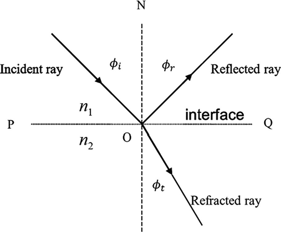
Gaussian optics, named after Carl Friedrich Gauss, is a technique in geometrical optics that describes the behavior of light rays in optical systems under the paraxial approximation. We take the opticalaxis to be along the z-axis, which is the general direction in which the rays travel, and our discussion is confined to those rays that lie in the x–z plane and that are close to the optical axis. In other words, only rays whose angular deviation from the optical axis is small are considered. These rays are called paraxial rays. Hence, the sine and tangent of the angles may be approximated by the angles themselves, that is, sintan . qq q »» Indeed, the mathematical treatment is simplified greatly because of the linearization process involved. For example, a linearized form of Snell’slawofrefraction, nnit12 sinsinff = , is nnit12 ff = . Figure 1.1-1 shows ray refraction for Snell’s law. fi and ft are the angles of incidence and refraction, respectively, which are measured from the normal, ON, to the interface POQ between Media 1 and 2. Media 1 and 2 are characterized by the constant refractive indices, n1 and n2 , respectively. In the figure, we also illustrate the lawofreflection, that is, ff ir = , where fr is the angleofreflection. Note that the incident ray, the refracted ray, and the reflected ray all lie in the same planeofincidence
Consider the propagation of a paraxial ray through an optical system as shown in Figure 1.1-2. A ray at a given z-plane may be specified by its height x from the optical axis and by its launching angle q. The convention for the angle is that q is measured in radians and is anticlockwise positive from the z-axis. The quantities ,x q () represent the
coordinates of the ray for a given z -plane However, instead of specifying the angle the ray makes with the z-axis, another convention is used. We replace the angle q by the corresponding vn = q , where n is the refractive index of the medium in which the ray is traveling. As we will see later, the use of this convention ensures that all the matrices involved are positive unimodular. A unimodularmatrix is a real square matrix with determinant +1 or −1, and a positive unimodular matrix has determinant +1.
To clarify the discussion, we let a ray pass through the input plane with the input raycoordinates (, ). xvn 11 11 = q After the ray passes through the optical system, we denote the outputraycoordinates (, ) xvn 22 22 = q on the output plane. In the paraxial approximation, the corresponding output quantities are linearly dependent on the input quantities. In other words, the output quantities can be expressed in terms of the weighted sum of the input quantities (known as the principleofsuperposition) as follows:
Figure 1.1-1 Geometry for Snell’s law and law of reflection
Figure 1.1-2 Ray propagating in an optical system
Figure 1.1-3 Ray propagating in a homogeneous medium with the input and output coordinates xvn 11 11 , = () q and xvn 22 22 ,, = () q respectively
xBvvCxDv 21 12 11 =+ =+ and, where A, B, C , and D are the weight factors. We can cast the above equations into a matrix form as
The ABCD matrix in Eq. (1.1-1) is called the raytransfermatrix, or the systemmatrix S , if it is represented by the multiplication of ray transfer matrices. In what follows, we shall derive several important ray transfer matrices.
1.1.1 Ray Transfer Matrices
Translation Matrix
A ray travels in a homogenous medium of refractive index n in a straight line (see Figure 1.1-3). Let us denote the input and output planes with the ray’s coordinates, and then we try to relate the input and output coordinates with a matrix after the traveling of the distance d Since nnn 12 == and qq qq 12 22 21 11 == == ,. vnnv From the geometry, we also find xxdxdxdvn 21 11
qq /. Therefore, we can relate the output coordinates of the ray with its input coordinates as follows:
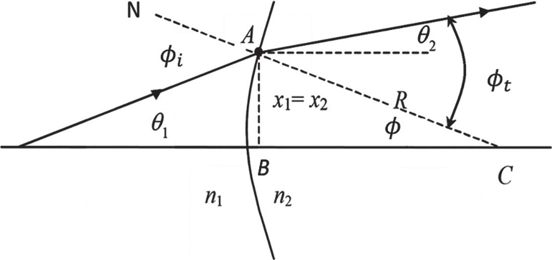
Figure 1.1-4 Ray trajectory during refraction at a spherical surface separating two regions of refractive indices n1 and n2
which is called the translationmatrix. The matrix describes the translation of a ray for a distance d along the optical axis in a homogenous medium of n The determinant of dn / is
and hence dn / is a positive unimodular matrix. For a translation of the ray in air, we have n = 1, and the translation can be represented simply by
Refraction Matrix
We consider a spherical surface separating two regions of refractive indices n1 and n2 as shown in Figure 1.1-4. The center of the spherical surface is at C, and its radius of curvature is R. The convention for the radiusofcurvature is as follows. The radius of curvature of the surface is taken to be positive (negative) if the center C of curvature lies to the right (left) of the surface. The ray strikes the surface at the point A and gets refracted into media n2 . Note that the input and output planes are the same. Hence, the height of the ray at A, before and after refraction, is the same, that is, xx21 = . fi and ft are the angles of incidence and refraction, respectively, which are measured from the normal NAC to the curved surface. Applying Snell’s law and using the paraxial approximation, we have
Now, from geometry, we know that φθ φ i =+ 1 and φθ φ t =+ 2 (Figure 1.1-4). Hence, the left side of Eq. (1.1-4) becomes
where we have used sin ff =≈ xR 1 /. Now, the right side of Eq. (1.1-4) is nnvnxR t 22 22 22 φθ φ =+ =+ () /, (1.1-6)
where xx12 = as the input and output planes are the same. Finally, putting Eqs. (1.1-5) and (1.1-6) into Eq. (1.1-4), we have vnxRvnxR 11 12 22 += + // or vvnnxRxx 21 12 11 2 =+ () = /, as (1.1-7)
We can formulate the above equation in terms of a matrix equation as
The determinant of R is
The 2 × 2 ray transfer matrix R is a positive unimodular matrix and is called the refractionmatrix. The matrix describes refraction for the spherical surface. The quantity p given by p nn R = 21 is called the refractingpower of the spherical surface. When R is measured in meters, the unit of p is called diopters. If an incident ray is made to converge on (diverge from) by a surface, the power is positive (negative) in sign.
Thick- and Thin-Lens Matrices
A thick lens consists of two spherical surfaces as shown in Figure 1.1-5. We shall find the system matrix that relates the system’s input coordinates xv11 , () to system’s output ray coordinates (, ). xv22 Let us first relate (, ) xv11 to (, ) xv11 ¢¢ through the spherical surface defined by R1 (, ) xv11 ¢¢ are the output coordinates due to the surface R1 According to Eq. (1.1-8), we have
Now, (, ) xv11 ¢¢ and (, ) xv22 ¢¢ are related through a translation matrix as follows:
where (, ) xv22 ¢¢ are the output coordinates after translation, which are also the coordinates of the input coordinates for the surface R2 . Finally, we relate (, ) xv22 ¢¢ to the system’s output coordinates (, ) xv22 through
If we now substitute Eq. (1.1-10) into Eq. (1.1-11), then we have
Subsequently, substituting Eq. (1.1-9) into the above equation, we have the system matrixequation of the entire system as follows:
We have now finally related the system’s input coordinates to output coordinates. Note that the system matrix, SR TR = RdnR 22 1 / , is a product of three ray transfer
Figure 1.1-5 Thick lens
matrices. In general, the system matrix is made up of a collection of ray transfer matrices to account for the effects of a ray passing through the optical system. As the ray goes from left to right in the positive direction of the z-axis, we obtain the system matrix by writing the ray transfer matrices from right to left. This is precisely the advantage of the matrix formalism in that any ray, during its propagation through the optical system, can be tracked by successive matrix multiplications. Let and be the 2 × 2 matrices as follows:
Then the rule of matrix multiplication is
Now, returning to the system matrix in Eq. (1.1-12), the determinant of the system matrix, SR TR = RdnR 22 1 / , is
Note that even the system matrix is also positive unimodular. The condition of a unit determinant is a necessary but not a sufficient condition on the system matrix. We now derive a matrix of an idea thin lens of focal length f , called the thin-lens matrix, f For a thin lens in air, we let d ® 0 and n1 1 = in the configuration of Figure 1.1-5. We also write nn 2 = for notational convenience. Then the system matrix in Eq. (1.1-12) becomes
where
For f > 0, we have a converging (convex) lens. On the other hand, we have a diverging (concave) lens when f < 0. Figure 1.1-6 summarizes the result for the ideal thin lens.
1.1-6 Ideal thin lens of focal length f and its associated ray transfer matrix
Note that the determinant of f is
1.1.2 Ray Tracing through a Thin Lens
As we have seen from Section 1.1.1, when a thin lens of focal length f is involved, then the matrix equation, from Eq. (1.1-13), is
Input Rays Traveling Parallel to the Optical Axis
From Figure 1.1-7a, we recognize that xx12 = as the heights of the input and output rays are the same for the thin lens. Now, according to Eq. (1.1-14), /.vxfv 21 1 =− + For v1 0 = , that is, the input rays are parallel to the optical axis, vxf 21 =− /. For positive , x1 v2 0 < as f > 0 for a converging lens. For negative , x1 v2 0. > All input rays parallel to the optical axis converge behind the lens to the back focal point (a distance of f away from the lens) of the lens as shown in Figure 1.1-7a. Note that for a thin lens, the front focal point is also a distance of f away from the lens.
Input Rays Traveling through the Center of the Lens
For input rays traveling through the center of the lens, their input ray coordinates are (, ), . xvv 11 1 0 = () The output ray coordinates, according to Eq. (1.1.14), are (, ), xvv 22 1 0 = () . Hence, we see as vv21 = , all rays traveling through the center of the lens will pass undeviated as shown in Figure 1.1-7b.
Figure
1.1-7
1.1-8
Input Rays Passing through the Front Focal Point of the Lens
For this case, the input ray coordinates are (, /)xvxf 11 1 = , and, according to Eq. (1.114), the output ray coordinates are (, ) xxv 21 2 0 == , which means that all output rays will be parallel to the optical axis () v2 0 = , as shown in Figure 1.1-7c.
Similarly, in the case of a diverging lens, we can draw conclusions as follows. The ray after refraction diverges away from the axis as if it were coming from a point on the axis a distance f in front of the lens, as shown in Figure 1.1-8a. The ray traveling through the center of the lens will pass undeviated, as shown in Figure 1.1-8b. Finally, for an input ray appearing to travel toward the back focus point of a diverging lens, the output ray will be parallel to the optical axis, as shown in Figure 1.1-8c
Example: Imaging by a Convex Lens
We consider a single-lens imaging as shown in Figure 1.1-9, where we assume the lens is immersed in air. We first construct a raydiagram for the imaging system. An object OO¢ is located a distance d0 in front of a thin lens of focal length f . We send two rays from a point O¢ towards the lens. Ray 1 from O¢ is incident parallel to the optical axis, and from Figure 1.1-7a, the input ray parallel to the optical axis converges behind the lens to the back focal point. A second ray, that is, ray 2 also from O¢, is now drawn through the center of the lens without bending and that is the result from Figure 1.1-7b. The interception of the two rays on the other side of the lens forms an image point of O¢. The image point of O¢ is labeled at I¢ in the diagram. The final image is real, inverted, and is called a realimage.
Figure
Ray tracing through a thin convex lens
(a) (b)
(c)
Figure
Ray tracing through a thin concave lens (a)
Now we investigate the imaging properties of the single thin lens using the matrix formalism. The input plane and the output plane of the optical system are shown in Figure 1.1-9. We let (, ) xv00 and (, ) xvii represent the coordinates of the ray at O¢ and I¢, respectively. We see there are three matrices involved in the problem. The overall system matrix equation becomes
The overall system matrix,
is expressed in terms of the product of three matrices written in order from right to left as the ray goes from left to right along the optical axis, as explained earlier. According to the rule of matrix multiplication, Eq. (1.1-15) can be simplified to
To investigate the conditions for imaging, let us concentrate on the ABCD matrix of in Eq. (1.1-16). In general, we see that xAxBvA ix =+ = 00 0 if B = 0, which means that all rays passing through the input plane at the same object point x0 will pass through the same image point xi in the output plane. This is the condition of imaging. In addition, for B = 0, Axx i = / 0 is defined as the lateralmagnification of
Figure 1.1-9 Ray diagram for single-lens imaging
Figure 1.1-10 Imaging of a converging lens with object inside the focal length
the imaging system. Now in our case of thin-lens imaging, B = 0 in Eq. (1.1-16) leads to ddddf ii00 0 +− = / , which gives the well-known thin-lensformula:
The sign convention for Eq. (1.1-17) is that the object distance d0 is positive (negative) if the object is to the left (right) of the lens. If the image distance di is positive (negative), the image is to the right (left) of the lens and it is real (virtual). In Figure 1.1-9, we have d0 0 > , di > 0, and the image is therefore real, which means physically that light rays actually converge to the formed image I¢. Hence, for imaging, Eq. (1.116) becomes
which relates the input ray and output ray coordinates in the imaging system. Using Eq. (1.1-17), the lateralmagnificationM of the imaging system is
The sign convention is that if M > 0, the image is erect, and if M < 0, the image is inverted. As shown in Figure 1.1-9, we have an inverted image as both di and d0 are positive.
If the object lies within the focal length, as shown in Figure 1.1-10, we follow the rules as given in Figure 1.1-8 to construct a ray diagram. However, now rays 1 and 2, after refraction by the lens, are divergent and do not intercept on the right side of the lens. They seem to come from a point I¢. In this case, since d0 0 > and di < 0 , M > 0. The final image is virtual, erect, and is called a virtualimage.
1.2 Resolution, Depth of Focus, and Depth of Field
1.2.1
Circular Aperture
The numericalaperture ( NA) of a lens is defined for an object or image located infinitely far away. Figure 1.2-1 shows an object located at infinity, which sends rays parallel to the lens with a circular aperture. The angle qim used to define the NA on the image side is
where ni is refractive index in the image space. Note that the aperturestop limits the angle of rays passing through the lens, which affects the achievable NA. Let us now find the lateral resolution, Dr
Since we treat light as particles in geometrical optics, each particle then can be characterized by its momentum, p0 . According to the uncertaintyprinciple in quantum mechanics, we relate the minimum uncertainty in a position of quantum, Dr , to the uncertainty of its momentum, Dpr , according to the relationship
where h is Planck’sconstant, and Dpr is the momentum spread in the r -component of the photons. The momentum of the FB ray (chief ray, a ray passes through the center of the lens) along the r-axis is zero, while the momentum of the FA ray (marginal ray, a ray passes through the edge of the lens) along the r-axis is ∆pp AB = 0 2 sin im (/ ) q , where ph00 = / l with l0 being the wavelength in the medium, that is, in the image space. Hence, Dpr is ∆∆ppp rAB ==22 2 0 sin im (/ ) q to accommodate a maximum variation (or spread) of the momentum direction by an angle qim. By substituting this into Eq. (1.2-2), we have lateralresolution Figure 1.2-1 Uncertainty principle used in finding lateral resolution and depth
Note that this equation reveals that in order to achieve high resolution, we can increase qim /2. For example, when qim /2 90 =° , Dr is half the wavelength, that is, / l0 2, which is the theoretical maximum lateral resolution. Since the wavelength in the image space, l0 , is equal to lvi n / , where l v is the wavelength in air or in vacuum, Eq. (1.2-3) becomes, using Eq. (1.2-1),
Similarly, we can calculate the depthoffocus, Dz . Depth of focus, also called longitudinalresolution in the image space, is the axial distance over which the image can be moved without loss of sharpness in the object. To find the depth of focus, we use
where Dpz is the momentum difference between rays FB and FA along the z-direction, as shown in Figure 1.2-1, which is given by
By substituting this expression into Eq. (1.2-5), we have
This equation reveals that in order to achieve small depth of focus, we can increase qim /2 . For example, when qim /2 90 =° , Dz is one wavelength, that is, l0 , which is the theoretical maximum longitudinal resolution. Equation (1.2-7) can be written in terms of the numerical aperture and is given by
For small angles, that is, qim << 1, one can use the approximation 11 2 22 −≈sinsinbb () / to get
Taking the equality in Eq. (1.2-9) and combining with Eq. (1.2-4), we have
Figure 1.2-2 Image-forming instrument illustrating resolutions in the object space and image space
under the small- NA approximation. This equality is derived from uncertainty relationship, which says that during imaging the higher the lateral resolution is, the shorter the depth of focus. For example, by increasing the lateral resolution by a factor of 2 will result in the depth of focus decreased by a factor of 4.
Figure 1.2-2 shows an image-forming instrument with qob and qim denoting the ray of maximum divergent angle and maximum convergent angle from the object side and the image side, respectively.
If the resolutions in the object space are given by ∆r v 00 2 ≈ l /NA and ∆znv 00 0 2 2 ≈ l /NA , where NA sin ob 00 2 = n (/ ) q and n0 is the refractive index in the object space, and if the lateral magnification of the instrument is M , the resolution on the image space is then ∆∆ rMr i ≈ 0 Let us establish the relationship between the depthoffield Dz0 and the depthoffocus Dzi , where ∆zniivi ≈ 2 2 l /NA with NA sin im ii n = (/ ) q 2 . Since ∆∆ rMrM iviv ≈= = ll // 2200 NA NA , we have NA NA 0 =×Mi . Hence,
This result indicates that the longitudinal resolutions in the object space and image space are related by a factor of M 2 . Take a 40×, NA 0 06 » . microscope objective as an example, we have ∆r v 0020 5 ≈≈ l /. NA mµ for red light with wavelength of 632 nm and the depth of field, ∆znv 00 0 2 23 5 ≈≈ l /. NA mµ for n0 1 = in air. In the image space, the lateral resolution is ∆∆ rMr i ≈= ×= 0 40 05 20 µµmm and the depth of focus is ∆∆ zMz i ≈= ×= 2 0 2 40 35 056 µmmm for ni = 1
1.2.2 Annular Aperture
Three-dimensional imaging in microscopy aims to develop techniques that can provide high lateral resolution, and at the same time maintain a large depth of focus in order to observe a thick specimen. However, calculations have shown that the depth of focus may be increased by reducing the numerical aperture of the lens, but this is achieved at the expense of a decrease in lateral resolution. In what follows, we
1.2-4 Uncertainty principle used in finding depth of focus for a lens with annular aperture stop
consider an annular aperture which has the property of increasing the depth of focus and at the same time maintaining the lateral resolution. An annularaperture is defined as a clear circular aperture with a central obstruction, as shown in Figure 1.2-3. If the aperture is an annulus with outer radius a and inner radius b, we define a central obscurationratio e = ba/. For e = 0 , we have a clear circular aperture.
Since bq = im as shown in Figure 1.2-1, the possible spread in the r-component of momentum Dpr is the same in Figure 1.2-4 as it is in Figure 1.2-1. Hence, the lateral resolution remains the same as that in the case of the clear aperture, that is, e = 0 , given by Eq. (1.2-4). However, the spread or uncertainty in the momentum in the zdirection is different due to the central obscuration of the annulus. Dpr in this case is the momentum difference between the ray passing the upper part of the annulus (Ray A) and the ray passing the lower part of the annulus (Ray B) and is given by
(1.2-12) where DpRay A and DpRay B are given by Eq. (1.2-6) with b and a substituted into the argument of cosine, respectively. Hence Eq. (1.2-12) becomes
Figure 1.2-3 Annular aperture
Figure
and the depth of focus is
which can be shown to have the form
where NA = ()sin/ b 2 , that is, assuming the lens is being immersed in air. For small NAs, it can be shown that Eq. (1.2-14) is given by
The above equation is consistent with Eq. (1.2-9) for a clear aperture, that is, for the case e = 0 . With 95% obstruction, that is, e = 095 . , we can increase the depth of focus of a clear lens by more than a factor of 10.
1.3
Illustrative Examples
1.3.1 Three-Dimensional Imaging through a Single-Lens Example
Figure 1.3-1a shows the imaging of two objects in front of the lens, where both of the object lie beyond the focal length of the lens. We note that magnification is different, depending on the object distance to the lens. Let us consider longitudinal magnification, M z , in addition to lateral magnification, M , considered earlier. Longitudinal magnification M z is the ratio of an image displacement along the axial direction, d di , to the corresponding object displacement, d d0 , that is, Mdd zi = dd / 0 .
Using Eq. (1.1-17) and treating di and d0 as variables, we take the derivative of di with respect to d0 to obtain
This equation is consistent with Eq. (1.2-11) and states that the longitudinal magnification is equal to the square of the lateral magnification. The minus sign in front of the equation signifies that a decrease in the distance of the object from the lens, d0 , will result in an increase in the image distance, di , and vice versa. The situation of a magnified volume is shown in Figure 1.3-1b, where a cube volume (abcd plus the dimension into the paper) is imaged into a truncated pyramid with a–b imaged into a '–b' and c–d imaged into c'–d'
Figure 1.3-1 (a) Illustration of different magnifications and (b) volumetric imaging
Figure 1.3-2 Spreading from a slit
1.3.2 Angle of Spread from a Slit Example
Consider light emanating from a slit aperture of width l x , as shown in Figure 1.3-2
We relate the minimum uncertainty in position Dx of a quantum to the uncertainty in its momentum Dp x according to