Students need to develop critical thinking skills in order to understand and evaluate the limitations of statistical methods. Understandable Statistics: Concepts and Methods makes students aware of method appropriateness, assumptions, biases, and justifiable conclusions.
CRITICAL THINKING
Unusual Values
Chebyshev’s theorem tells us that no matter what the data distribution looks like, at least 75% of the data will fall within 2 standard deviations of the mean. As we will see in Chapter 6, when the distribution is mound-shaped and symmetric, about 95% of the data are within 2 standard deviations of the mean. Data values beyond 2 standard deviations from the mean are less common than those closer to the mean.
In fact, one indicator that a data value might be an outlier is that it is more than 2.5 standard deviations from the mean (Source: Statistics, by G. Upton and I. Cook, Oxford University Press).
UNUSUAL VALUES
For a binomial distribution, it is unusual for the number of successes r to be higher than m 1 2.5s or lower than m 2.5s
We can use this indicator to determine whether a specified number of successes out of n trials in a binomial experiment are unusual.
For instance, consider a binomial experiment with 20 trials for which probability of success on a single trial is p 5 0 70 The expected number of successes is m 5 14, with a standard deviation of s < 2 A number of successes above 19 or below 9 would be considered unusual However, such numbers of successes are possible
interpretation
increasingly, calculators and computers are used to generate the numeric results of a statistical process. However, the student still needs to correctly interpret those results in the context of a particular application. the interpretation feature calls attention to this important step. interpretation is stressed in examples, in guided exercises, and in the problem sets.
Critical thinking
Critical thinking is an important skill for students to develop in order to avoid reaching misleading conclusions. the Critical thinking feature provides additional clarification on specific concepts as a safeguard against incorrect evaluation of information.
SOLUTION: Since we want to know the number of standard deviations from the mean, we want to convert 6.9 to standard z units.
Interpretation The amount of cheese on the selected pizza is only 2.20 standard deviations below the mean. The fact that z is negative indicates that the amount of cheese is 2.20 standard deviations below the mean. The parlor will not lose its franchise based on this sample.
6. Interpretation A campus performance series features plays, music groups, dance troops, and stand-up comedy The committee responsible for selecting the performance groups include three students chosen at random from a pool of volunteers. This year the 30 volunteers came from a variety of majors. However, the three students for the committee were all music majors. Does this fact indicate there was bias in the selection process and that the selection process was not random? Explain.
7. Critical Thinking Greg took a random sample of size 100 from the population of current season ticket holders to State College men’s basketball games. Then he took a random sample of size 100 from the population of current season ticket holders to State College women’s basketball games.
(a) venience, random) did Greg use to sample from the population of current season ticket holders to all State College basketball games played by either men or women?
Critical thinking and interpretation exercises
in every section and chapter problem set, Critical thinking problems provide students with the opportunity to test their understanding of the application of statistical methods and their interpretation of their results. interpretation problems ask students to apply statistical results to the particular application.
(b) Is it appropriate to pool the samples and claim to have a random sample of size 200 from the population of current season ticket holders to all State College home basketball games played by either men or women? Explain. vii
Statistical literacy
no language, including statistics, can be spoken without learning the vocabulary. Understandable Statistics: Concepts and Methods introduces statistical terms with deliberate care.
What Does the Level of Measurement Te ll Us ?
The level of measurement tells us which arithmetic processes are appropriate for the data This is important because different statistical processes require various kinds of arithmetic. In some instances all we need to do is count the number of data that meet specified criteria In such cases nominal (and higher) data levels are all appropriate. In other cases we need to order the data, so nominal data would not be suitable Many other statistical processes require division, so data need to be at the ratio level. Just keep the nature of the data in mind before beginning statistical computations
important features of a (concept, method, or result)
in statistics we use many different types of graphs, samples, data, and analytical methods. the features of each such tool help us select the most appropriate ones to use and help us interpret the information we receive from applications of the tools.
what does (concept, method, statistical result) tell Us?
this feature gives a brief summary of the information we obtain from the named concept, method, or statistical result.
Important Fe a tures of a Simple Random Sampl e
For a simple random sample
• n from the population has an equal chance of being selected.
• No researcher bias occurs in the items selected for the sample.
• For instance, from a population of 10 cats and 10 dogs, a random sample of size 6 could consist of all cats.
definition Boxes
Whenever important terms are introduced in text, blue definition boxes appear within the discussions. these boxes make it easy to reference or review terms as they are used further.
statistical literacy problems
in every section and chapter problem set, Statistical literacy problems test student understanding of terminology, statistical methods, and the appropriate conditions for use of the different processes.
Box-and-Whisker Plots
The quartiles together with the low and high data values give us a very useful number summary of the data and their spread.
FIVE-NUMBER SUMMARY
Lowest value, Q1, median, Q3, highest value
box-and-whisker plot
Box-and-whisker plots provide another useful technique from exploratory data analysis (E DA) for describing data
SECTION 4.1
Probability of an event A, P(A) 144
Intuition 144
Relative frequency 144
Equally likely outcomes 144
Law of large numbers 146
Statistical experiment 146
Event 146
Simple event 146
Sample space 146
Complement of event Ac 148
SECTION 4.2
Independent events 156
Dependent events 156
Probability of A and B 156
Event A | B 156
Conditional probability 156
P 1 A | B 2 156
linking Concepts: writing projects
much of statistical literacy is the ability to communicate concepts effectively. the linking Concepts: Writing Projects feature at the end of each chapter tests both statistical literacy and critical thinking by asking the student to express their understanding in words.
Multiplication rules of probability (for independent and dependent events) 156
More than two independent events 161
Probability of A or B 161
Event A and B 161
Event A or B 161
Mutually exclusive events 163
Addition rules (for mutually exclusive and general events) 163
More than two mutually exclusive events 165
Basic probability rules 168
SECTION 4.3
Multiplication rule of counting 177
Tree diagram 178
Factorial notation 181
Permutations rule 181
Combinations rule 183
LINKING CONCEPTS: WRITING PROJECTS
important words & symbols
the important Words & Symbols within the Chapter Review feature at the end of each chapter summarizes the terms introduced in the Definition Boxes for student review at a glance. Page numbers for first occurrence of term are given for easy reference.
Discuss each of the following topics in class or review the topics on your own. Then write a brief but complete essay in which you summarize the main points. Please include formulas and graphs as appropriate.
1. What does it mean to say that we are going to use a sample to draw an inference about a population? Why is a random sample so important for this process? If we wanted a random sample of students in the cafeteria, why couldn’ t we just choose the students who order Diet Pepsi with their lunch? Comment on the statement, “A random sample is like a miniature population, whereas samples that are not random are likely to be biased.” Why would the students who order Diet Pepsi with lunch not be a random sample of students in the cafeteria?
2. In your own words, explain the differences among the following samplingter sample, multistage sample, and convenience sample. Describe situations in which each type might be useful.
5. Basic Computation: Central Limit Theorem Suppose x has a distribution with a mean of 8 and a standard deviation of 16. Random samples of size n 5 64 are drawn.
(a) Describe the x distribution and compute the mean and standard deviation of the distribution.
(b) Find the z value corresponding to x 5 9
(c) Find P 1 x 7 9 2 .
(d) Interpretation Would it be unusual for a random sample of size 64 from the x distribution to have a sample mean greater than 9? Explain.
Basic Computation problems
these problems focus student attention on relevant formulas, requirements, and computational procedures. After practicing these skills, students are more confident as they approach real-world applications.
30. Expand Your Knowledge: Geometric Mean When data consist of percentages, ratios, compounded growth rates, or other rates of change, the geometric mean is a useful measure of central tendency. For n data values,
expand your Knowledge problems
expand your Knowledge problems present optional enrichment topics that go beyond the material introduced in a section. vocabulary and concepts needed to solve the problems are included at point-of-use, expanding students’ statistical literacy.
Geometric mean 5 1 n product of the n data values, assuming all data values are positive average growth factor over 5 years of an investment in a mutual -
metric mean of 1.10, 1.12, 1.148, 1.038, and 1.16. Find the average growth factor of this investment
Direction and Purpose
Real knowledge is delivered through direction, not just facts. Understandable Statistics: Concepts and Methods ensures the student knows what is being covered and why at every step along the way to statistical literacy.
Chapter preview Questions
Preview Questions at the beginning of each chapter give the student a taste of what types of questions can be answered with an understanding of the knowledge to come.
Normal Curves and Sampling Distributions
PREVIEW QUESTIONS
PART I
What are some characteristics of a normal distribution? What does the empirical rule tell you about data spread around the mean? How can this information be used in quality control? (SECTION 6.1)
Can you compare apples and oranges, or maybe elephants and butterflies? In most cases, the answer is no unless you first standardize your measurements What are a standard normal distribution and a standard z score? (SECTION 6.2)
How do you convert any normal distribution to a standard normal distribution? How do you find probabilities of “standardized events”? (SECTION 6.3)
PART II
FOCUS PROBLEM
Benford’s Law: The Importance of Being Number 1
As humans, our experiences are finite and limited. Consequently, most of the important decisions in our lives are based on sample (incomplete) information. What is a probability sampling distribution? How will sampling distributions help us make good decisions based on incomplete information? (SECTION 6.4)
There is an old saying: All roads lead to Rome. In statistics, we could recast this saying: All probability distributions average out to be normal distributions (as the sample size increases). How can we take advantage of this in our study of sampling distributions? (SECTION 6 5)
Benford’s Law states that in a wide variety of circumdisproportionately often. Benford’s Law applies to such diverse topics as the drainage areas of rivers; properties of magazines, and government reports; and the half-lives of radioactive atoms!
The binomial and normal distributions are two of the most important probability distributions in statistics. Under certain limiting condi-
“1” about 30% of the time, with “2” about 18% of time, and with “3” about 12.5% of the time. Larger digits occur less often. For example, less than 5% of the numbers in circumstances such as these begin with the digit 9. This is in dramatic contrast to a random sampling situation, in which each of the digits 1 through 9 has an equal chance of appearing.
▲ Chapter focus problems
the Preview Questions in each chapter are followed by a Focus Problem, which serves as a more specific example of what questions the student will soon be able to answer. the Focus Problems are set within appropriate applications and are incorporated into the end-of-section exercises, giving students the opportunity to test their understanding.
x
8. Focus Problem: Benford’s Law Again, suppose you are the auditor for a veryputer data bank (see Problem 7). You draw a random sample of n 5 228 numbers r 5 92 p represent the popu-
i. Test the claim that p is more than 0.301. Use a 5 0 01.
ii. If p is in fact larger than 0.301, it would seem there are too many num-
from the point of view of the Internal Revenue Service. Comment from the perspective of the Federal Bureau of Investigation as it looks for
iii. Comment on the following statement: “If we reject the null hypothesis at a, we have not proved H0 to be false. We can say that the probability is a that we made a mistake in rejecting H0.” Based on the outcome of the test, would you recommend further investigation before accusing the company of fraud?
Pressmaster/Shutterstock.com
focus points
each section opens with bulleted Focus Points describing the primary learning objectives of the section.
Measures of Central Tendency: Mode, Median, and Mean
FOCUS POINTS
• Compute mean, median, and mode from raw data.
• Interpret what mean, median, and mode tell you.
• Explain how mean, median, and mode can be affected by extreme data values
• What is a trimmed mean? How do you compute it?
• Compute a weighted average
The average price of an ounce of gold is $1350. The Zippy car averages 39 miles per gallon on the highway A survey showed the average shoe size for women is size 9.
In each of the preceding statements, one number is used to describe the entire sample or population. Such a number is called an average There are many ways to compute averages, but we will study only three of the major ones.
The easiest average to compute is the mode
The mode of a data set is the value that occurs most frequently Note: If a data set has no single value that occurs more frequently than any other, then that data set has no mode
Mode
the letters in each word of this sentence and give the mode. The numbers of letters in the words of the sentence are
LOOKING FORWARD
In later chapters we will use information based on a sample and sample statistics to estimate population parameters (Chapter 7) or make decisions about the value of population parameters (Chapter 8).
looking forward
this feature shows students where the presented material will be used later. it helps motivate students to pay a little extra attention to key topics.
CHAPTER REVIEW
In this chapter, you’ve seen that statistics is the study of how to collect, organize, analyze, and interpret numerical information from populations or samples This chapter discussed some of the features of data and ways to collect data. In particular, the chapter discussed
• Individuals or subjects of a study and the variables associated with those individuals
• levels of measurement of data
• Sample and population data. Summary measurements from sample data are called statistics, and those from populations are called parameters.
▲ Chapter summaries
• Sampling strategies, including simple random, Inferential techniques presented in this text are based on simple random samples.
• Methods of obtaining data: Use of a census, simulation, observational studies, experiments, and surveys
• Concerns: Undercoverage of a population, nonresponse, bias in data from surveys and other factors, effects of confounding or lurking variables on other variables, generalization of study results beyond the population of the study, and study sponsorship
the Summary within each Chapter Review feature now also appears in bulleted form, so students can see what they need to know at a glance.
section can be covered quickly
include The Story of Old Faithful in Data Highlights, Problem 1; Linking Concepts, Problem 1; and the trade winds of Hawaii (Using Technology).
EXAMPLE 1
Real-World Skills
Statistics is not done in a vacuum. Understandable Statistics: Concepts and Methods gives students valuable skills for the real world with technology instruction, genuine applications, actual data, and group projects.
Tech Notes >
ReviSeD! tech notes
tech notes appearing throughout the text give students helpful hints on using ti84Plus and ti-nspire (with ti-84Plus keypad) and ti-83Plus calculators, microsoft excel 2013, minitab, and minitab express to solve a problem. they include display screens to help students visualize and better understand the solution.
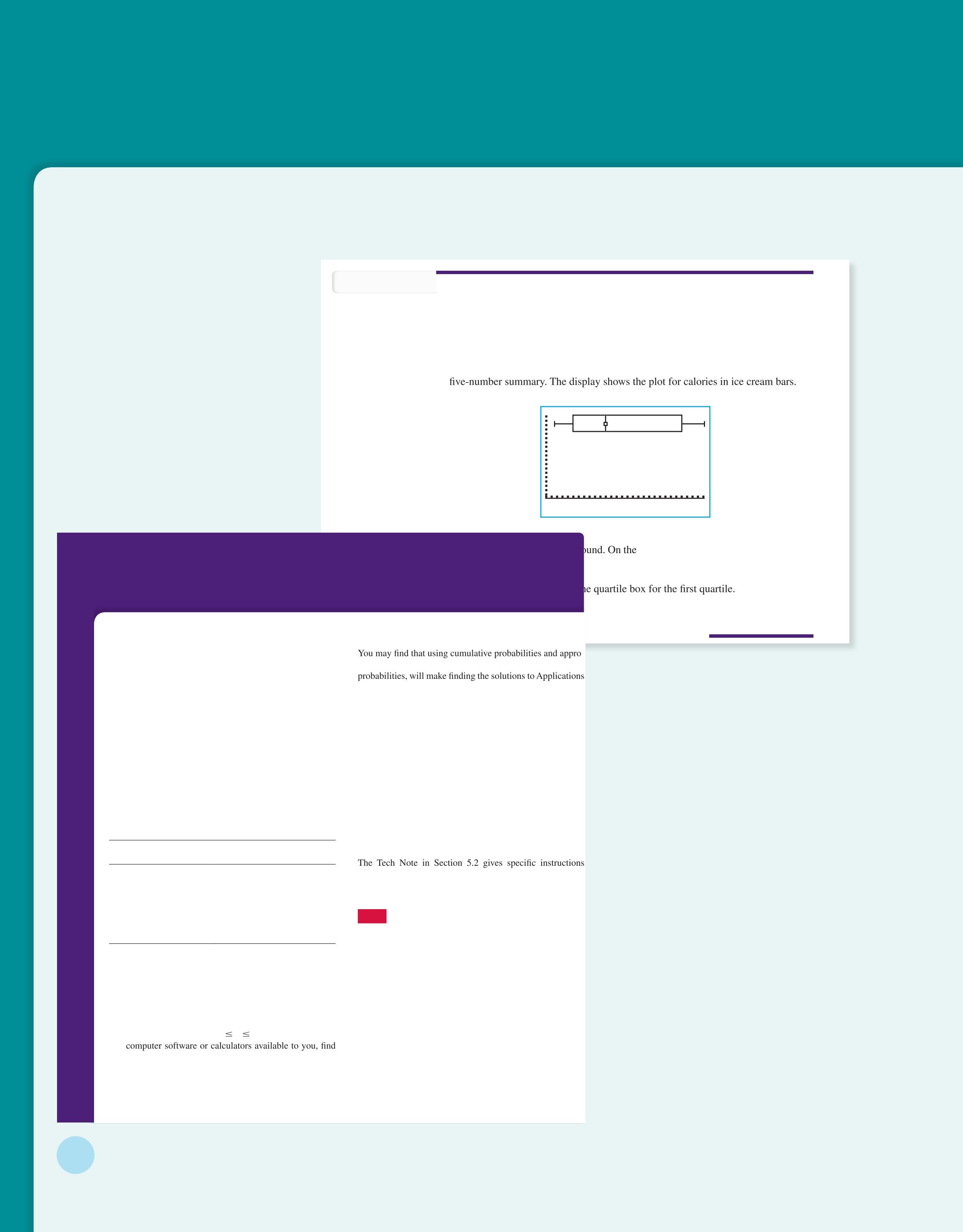
Box-and-Whisker Plot
Both Minitab and the TI-84Plus/TI-83Plus/TI-nspire calculators support boxand-whisker plots. On the TI-84Plus/TI-83Plus/TI-nspire, the quartiles Q1 and Q3 are calculated as we calculate them in this text. In Minitab and Excel 2013, they are calculated using a slightly different process.
TI-84Plus/TI-83Plus/TI-nspire (with TI-84Plus Keypad) Press STATPLOT ➤On. Highlight box plot. Use Trace and the arrow keys to display the values of the
USING TECHNOLOGY
Binomial Distributions
Although tables of binomial probabilities can be found in most libraries, such tables are often inadequate. Either the value of p (the probability of success on a trial) you are looking for is not in the table, or the value of n (the number of trials) you are looking for is too large for the table. In Chapter 6, we will study the normal approximation to the binomial. This approximation is a great help in many practical applications. Even so, we sometimes use the formula for the binomial probability distribution on a computer or graphing calculator to compute the probability we want.
Applications
The following percentages were obtained over many years of observation by the U.S. Weather Bureau. All data listed are for the month of December
Location Long-Term Mean % of Clear Days in Dec
Juneau, Alaska 18%
Seattle, Washington 24%
Hilo, Hawaii 36%
Honolulu, Hawaii 60%
Las Vegas, Nevada 75%
Phoenix, Arizona 77%
Adapted from Local Climatological Data, U.S Weather Bureau publication, “Normals, Means, and Extremes” Table.
In the locations listed, the month of December is a relatively stable month with respect to weather Since weather patterns from one day to the next are more or less the same, it is reasonable to use a binomial probability model.
1. Let r be the number of clear days in December Since December has 31 days, 0 r 31 Using appropriate the probability P(r) for each of the listed locations when r 0, 1, 2, . . , 31
2. For each location, what is the expected value of the probability distribution? What is the standard deviation?
Excel 2013 Does not produce box-and-whisker plot. However, each value of the Home ribbon, click the Insert Function fx In the dialogue box, select Statistical as the category and scroll to Quartile In the dialogue box, enter the data location and then enter the number of the value you
Minitab Press Graph ➤ Boxplot In the dialogue box, set Data View to IQRange Box MinitabExpress Press Graph ➤ Boxplot ➤ simple.
priate subtraction of probabilities, rather than addition of
3 to 7 easier
3. Estimate the probability that Juneau will have at most 7 clear days in December
4. Estimate the probability that Seattle will have from 5 to 10 (including 5 and 10) clear days in December
5. Estimate the probability that Hilo will have at least 12 clear days in December
6. Estimate the probability that Phoenix will have 20 or more clear days in December
7. Estimate the probability that Las Vegas will have from 20 to 25 (including 20 and 25) clear days in December Technology Hints
TI-84Plus/TI-83Plus/TI-nspire (with TI-84 Plus keypad), Excel 2013, Minitab/MinitabExpress
for binomial distribution functions on the TI-84Plus/ TI-83Plus/TI-nspire (with TI-84Plus keypad) calculators, Excel 2013, Minitab/MinitabExpress, and SPSS.
SPSS
In SPSS, the function PDF.BINOM(q,n,p) gives the probability of q successes out of n trials, where p is the probability of success on a single trial. In the data editor, name a variable r and enter values 0 through n. Name another variable Prob_r Then use the menu choices Transform ➤ Compute In the dialogue box, use Prob_r for the target variable. In the function group, select PDF and Noncentral PDF In the function box, select PDF.BINOM(q,n,p) Use the variable r for q and appropriate values for n and p. Note that the function CDF.BINOM(q,n,p), from the CDF and Noncentral CDF group, gives the cumulative probability of 0 through q successes.
ReviSeD! Using technology
Further technology instruction is available at the end of each chapter in the Using technology section. Problems are presented with real-world data from a variety of disciplines that can be solved by using ti-84Plus and ti-nspire (with ti-84Plus keypad) and ti-83Plus calculators, microsoft excel 2013, minitab, and minitab express.
Central Limit Theorem
A certain strain of bacteria occurs in all raw milk. Let x be the bacteria count per milliliter of milk. The health department has found that if the milk is not contaminated, then x has a distribution that is more or less mound-shaped and symmetric. The mean of the x distribution is m 5 2500, and the standard deviation is s 5 300 In a large commercial dairy, the health inspector takes 42 random samples of the milk produced each day At the end of the day, the bacteria count in each of the 42 samples is averaged to obtain the sample mean bacteria count x
(a) Assuming the milk is not contaminated, what is the distribution of x?
SOLUTION: The sample size is n 5 42 Since this value exceeds 30, the central limit theorem applies, and we know that x will be approximately normal, with mean and standard deviation
most exercises in each section are applications problems.
DATA HIGHLIGHTS: GROUP PROJECTS
FIGURE 2-20
UPDAteD! applications
Real-world applications are used from the beginning to introduce each statistical process. Rather than just crunching numbers, students come to appreciate the value of statistics through relevant examples.
11. Pain Management: Laser Therapy “Effect of Helium-Neon Laser Auriculotherapy on Experimental Pain Threshold” is the title of an article in the journal Physical Therapy (Vol. 70, No. 1, pp. 24–30). In this article, laser therapy was discussed as a useful alternative to drugs in pain management of chronically ill patients. To measure pain threshold, a machine was used that delivered low-voltage direct current to different parts of the body (wrist, neck, and back). The machine measured current in milliamperes (mA). The pretreatment detectable) at m 5 3.15 mA with standard deviation s 5 1.45 mA. Assume that the distribution of threshold pain, measured in milliamperes, is symmetric and more or less mound-shaped. Use the empirical rule to
(a) estimate a range of milliamperes centered about the mean in which about 68% of the experimental group had a threshold of pain.
(b) estimate a range of milliamperes centered about the mean in which about 95% of the experimental group had a threshold of pain.
12. Control Charts: Yellowstone National Park Yellowstone Park Medical Services (YPMS) provides emergency health care for park visitors. Such health care includes treatment for everything from indigestion and sunburn to more serious injuries. A recent issue of Yellowstone Today (National Park
Break into small groups and discuss the following topics. Organize a brief outline in which you summarize the main points of your group discussion.
1.Examine Figure 2-20, “Everyone Agrees: Slobs Make Worst Roommates.”
This is a clustered bar graph because two percentages are given for each response category: responses from men and responses from women. Comment about how the artistic rendition has slightly changed the format of a bar graph. Do the bars seem to have lengths that accurately the relative percentages of the responses? In your own opinion, does the artistic rendition enhance or confuse the information? Explain. Which characteristic of “worst roommates” does the graphic seem to illustrate? Can this graph be considered a Pareto chart for men? for women? Why or why not? From the information given in theure, do you think the survey just listed the four given annoying characteristics? Do you think a respondent could choose more than one characteristic? Explain
Source: Advantage Business Research for Mattel Compatibility
data highlights: Group projects
Using group Projects, students gain experience working with others by discussing a topic, analyzing data, and collaborating to formulate their response to the questions posed in the exercise.
making the Jump
get to the “Aha!” moment faster. Understandable Statistics: Concepts and Methods provides the push students need to get there through guidance and example.
PROCEDURE
How to test M when S is known
Requirements
Let x be a random variable appropriate to your application. Obtain a simple random sample (of size n) of x values from which you compute the sample mean x The value of s is already known (perhaps from a previous study). If you can assume that x has a normal distribution, then any sample size n will work. If you cannot assume this, then use a sample size n 30.
Procedure
1. In the context of the application, state the null and alternate hypotheses and set the a.
2. Use the known s, the sample size n, the value of x from the sample, and m from the null hypothesis to compute the standardized sample test statistic
z 5 x m s 1n
procedures and Requirements
Procedure display boxes summarize simple step-by-step strategies for carrying out statistical procedures and methods as they are introduced. Requirements for using the procedures are also stated. Students can refer back to these boxes as they practice using the procedures.
GUIDED EXERCISE 11
Probability Regarding x
3. Use the standard normal distribution and the type of test, one-tailed or P-value corresponding to the test statistic.
4. Conclude the test. If P-value a, then reject H0. If P-value 7 a, then do not reject H0.
5. Interpret your conclusion in the context of the application.
In mountain country, major highways sometimes use tunnels instead of long, winding roads over high passes. However, too many vehicles in a tunnel at the same time can cause a hazardous situation Traffic engineers are studying a long tunnel in Colorado. If x represents the time for a vehicle to go through the tunnel, it is known that the x distribution has mean m 5 12.1 minutes and standard deviation s 5 3.8 minutes under ordinary traffic conditions From a histogram of x values, it was found that the x distribution is mound-shaped with some symmetry about the mean Engineers have calculated that, on average, vehicles should spend from 11 to 13 minutes in the tunnel. If the time is less than 11 minutes, traffic is moving too fast for safe travel in the tunnel. If the time is more than 13 minutes, there is a problem of bad air quality (too much carbon monoxide and other pollutants).
Under ordinary conditions, there are about 50 vehicles in the tunnel at one time. What is the probability that the mean time for 50 vehicles in the tunnel will be from 11 to 13 minutes?
We will answer this question in steps
(a) Let x represent the sample mean based on samples of size 50. Describe the x distribution.
Guided exercises
Students gain experience with new procedures and methods through guided exercises. Beside each problem in a guided exercise, a completely worked-out solution appears for immediate reinforcement.
(b) Find P 1 11 6 x 6 13 2
(c) Interpret your answer to part (b).
From the central limit theorem, we expect the x distribution to be approximately normal, with mean and standard deviation mx 5 m 5 12.1 sx 5 s 1n 5 3.8 150 < 0.54
We convert the interval 11 6 x 6 13
to a standard z interval and use the standard normal probability table to find our answer Since
z 5 x m s/ 1n < x 12.1 0.54 x 5 11 converts to z < 11 12.1 0.54 5 2.04 and x 5 13 converts to z < 13 12.1 0.54 5 1.67
Therefore, P 1 11 6 x 6 13 2 5 P 1 2.04 6 z 6 1.67 2
5 0.9525 0.0207
5 0.9318
It seems that about 93% of the time, there should be no safety hazard for average traffic flow
Preface
Welcome to the exciting world of statistics! We have written this text to make statistics accessible to everyone, including those with a limited mathematics background. Statistics affects all aspects of our lives. Whether we are testing new medical devices or determining what will entertain us, applications of statistics are so numerous that, in a sense, we are limited only by our own imagination in discovering new uses for statistics.
Overview
The twelfth edition of Understandable Statistics: Concepts and Methods continues to emphasize concepts of statistics. Statistical methods are carefully presented with a focus on understanding both the suitability of the method and the meaning of the result. Statistical methods and measurements are developed in the context of applications.
Critical thinking and interpretation are essential in understanding and evaluating information. Statistical literacy is fundamental for applying and comprehending statistical results. In this edition we have expanded and highlighted the treatment of statistical literacy, critical thinking, and interpretation.
We have retained and expanded features that made the first 11 editions of the text very readable. Definition boxes highlight important terms. Procedure displays summarize steps for analyzing data. Examples, exercises, and problems touch on applications appropriate to a broad range of interests.
The twelfth edition continues to have extensive online support. Instructional videos are available on DVD. The companion web site at http://www.cengage.com/ statistics/brase contains more than 100 data sets (in JMP, Microsoft Excel, Minitab, SPSS, and TI-84Plus/TI-83Plus/TI-nspire with TI-84Plus keypad ASCII file formats) and technology guides.
Available with the twelfth edition is MindTap for Introductory Statistics. MindTap for Introductory Statistics is a digital-learning solution that places learning at the center of the experience and can be customized to fit course needs. It offers algorithmically-generated problems, immediate student feedback, and a powerful answer evaluation and grading system. Additionally, it provides students with a personalized path of dynamic assignments, a focused improvement plan, and just-in-time, integrated review of prerequisite gaps that turn cookie cutter into cutting edge, apathy into engagement, and memorizers into higher-level thinkers.
MindTap for Introductory Statistics is a digital representation of the course that provides tools to better manage limited time, stay organized and be successful. Instructors can customize the course to fit their needs by providing their students with a learning experience—including assignments—in one proven, easy-to-use interface.
With an array of study tools, students will get a true understanding of course concepts, achieve better grades, and set the groundwork for their future courses. These tools include:
• A Pre-course Assessment—a diagnostic and follow-up practice and review opportunity that helps students brush up on their prerequisite skills to prepare them to succeed in the course.
• Just-in-time and side-by-side assignment help –provide students with scaffolded and targeted help, all within the assignment experience, so everything the student needs is in one place.
• Stats in Practice—a series of 1-3 minute news videos designed to engage students and introduce each unit by showing them how that unit’s concepts are practically used in the real world. Videos are accompanied by follow-up questions to reinforce the critical thinking aspect of the feature and promote in-class discussion. Learn more at www.cengage.com/mindtap.
Major Changes in the Twelfth Edition
With each new edition, the authors reevaluate the scope, appropriateness, and effectiveness of the text’s presentation and reflect on extensive user feedback. Revisions have been made throughout the text to clarify explanations of important concepts and to update problems.
Additional Flexibility Provided by Dividing Chapters into Parts
In the twelfth edition several of the longer chapters have been broken into easy to manage and teach parts. Each part has a brief introduction, brief summary, and list of end-of-chapter problems that are applicable to the sections in the specified part. The partition gives appropriate places to pause, review, and summarize content. In addition, the parts provide flexibility in course organization.
Chapter 6 Normal Distributions and Sampling Distributions: Part I discusses the normal distribution and use of the standard normal distribution while Part II contains sampling distributions, the central limit theorem, and the normal approximation to the binomial distribution.
Chapter 7 Estimation: Part I contains the introduction to confidence intervals and confidence intervals for a single mean and for a single proportion while Part II has confidence intervals for the difference of means and for the difference of proportions.
Chapter 8 Hypothesis Testing: Part I introduces hypothesis testing and includes tests of a single mean and of a single proportion. Part II discusses hypothesis tests of paired differences, tests of differences between two means and differences between two proportions.
Chapter 9 Correlation and Regression: Part I has simple linear regression while Part II has multiple linear regression.
Revised Examples and New Section Problems
Examples and guided exercises have been updated and revised. Additional section problems emphasize critical thinking and interpretation of statistical results.
Updates in Technology Including Mindtab Express
Instructions for Excel 2013, Minitab 17 and new Minitab Express are included in the Tech Notes and Using Technology
Continuing Content
Critical Thinking, Interpretation, and Statistical Literacy
The twelfth edition of this text continues and expands the emphasis on critical thinking, interpretation, and statistical literacy. Calculators and computers are very good at providing numerical results of statistical processes. However, numbers from a computer or calculator display are meaningless unless the user knows how to interpret the results and if the statistical process is appropriate. This text helps students determine whether or not a statistical method or process is appropriate. It helps
students understand what a statistic measures. It helps students interpret the results of a confidence interval, hypothesis test, or liner regression model.
Introduction of Hypothesis Testing Using P-Values
In keeping with the use of computer technology and standard practice in research, hypothesis testing is introduced using P-values. The critical region method is still supported but not given primary emphasis.
Use of Student’s t Distribution in Confidence Intervals and Testing of Means
If the normal distribution is used in confidence intervals and testing of means, then the population standard deviation must be known. If the population standard deviation is not known, then under conditions described in the text, the Student’s t distribution is used. This is the most commonly used procedure in statistical research. It is also used in statistical software packages such as Microsoft Excel, Minitab, SPSS, and TI-84Plus/TI-83Plus/TI-nspire calculators.
Confidence Intervals and Hypothesis Tests of Difference of Means
If the normal distribution is used, then both population standard deviations must be known. When this is not the case, the Student’s t distribution incorporates an approximation for t, with a commonly used conservative choice for the degrees of freedom. Satterthwaite’s approximation for the degrees of freedom as used in computer software is also discussed. The pooled standard deviation is presented for appropriate applications (s1 < s2).
Features in the Twelfth Edition Chapter and Section Lead-ins
• Preview Questions at the beginning of each chapter are keyed to the sections.
• Focus Problems at the beginning of each chapter demonstrate types of questions students can answer once they master the concepts and skills presented in the chapter.
• Focus Points at the beginning of each section describe the primary learning objectives of the section.
Carefully Developed Pedagogy
• Examples show students how to select and use appropriate procedures.
• Guided Exercises within the sections give students an opportunity to work with a new concept. Completely worked-out solutions appear beside each exercise to give immediate reinforcement.
• Definition boxes highlight important definitions throughout the text.
• Procedure displays summarize key strategies for carrying out statistical procedures and methods. Conditions required for using the procedure are also stated.
• What Does (a concept, method or result) Tell Us? summarizes information we obtain from the named concepts and statistical processes and gives insight for additional application.
• Important Features of a (concept, method, or result) summarizes the features of the listed item.
• Looking Forward features give a brief preview of how a current topic is used later.
• Labels for each example or guided exercise highlight the technique, concept, or process illustrated by the example or guided exercise. In addition, labels for section and chapter problems describe the field of application and show the wide variety of subjects in which statistics is used.
• Section and chapter problems require the student to use all the new concepts mastered in the section or chapter. Problem sets include a variety of real-world applications with data or settings from identifiable sources. Key steps and solutions to odd-numbered problems appear at the end of the book.
• Basic Computation problems ask students to practice using formulas and statistical methods on very small data sets. Such practice helps students understand what a statistic measures.
• Statistical Literacy problems ask students to focus on correct terminology and processes of appropriate statistical methods. Such problems occur in every section and chapter problem set.
• Interpretation problems ask students to explain the meaning of the statistical results in the context of the application.
• Critical Thinking problems ask students to analyze and comment on various issues that arise in the application of statistical methods and in the interpretation of results. These problems occur in every section and chapter problem set.
• Expand Your Knowledge problems present enrichment topics such as negative binomial distribution; conditional probability utilizing binomial, Poisson, and normal distributions; estimation of standard deviation from a range of data values; and more.
• Cumulative review problem sets occur after every third chapter and include key topics from previous chapters. Answers to all cumulative review problems are given at the end of the book.
• Data Highlights and Linking Concepts provide group projects and writing projects.
• Viewpoints are brief essays presenting diverse situations in which statistics is used.
• Design and photos are appealing and enhance readability.
Technology Within the Text
• Tech Notes within sections provide brief point-of-use instructions for the TI-84Plus, TI-83Plus, and TI-nspire (with 84Plus keypad) calculators, Microsoft Excel 2013, and Minitab.
• Using Technology sections show the use of SPSS as well as the TI-84Plus, TI-83Plus, and TI-nspire (with TI-84Plus keypad) calculators, Microsoft Excel, and Minitab.
Interpretation Features
To further understanding and interpretation of statistical concepts, methods, and results, we have included two special features: What Does (a concept, method, or result) Tell Us? and Important Features of a (concept, method, or result). These features summarize the information we obtain from concepts and statistical processes and give additional insights for further application.
Expand Your Knowledge Problems and Quick Overview Topics With Additional Applications
Expand Your Knowledge problems do just that! These are optional but contain very useful information taken from the vast literature of statistics. These topics are not included in the main text but are easily learned using material from the section or previous sections. Although these topics are optional, the authors feel they add depth and enrich a student’s learning experience. Each topic was chosen for its relatively straightforward presentation and useful applications. All such problems and their applications are flagged with a sun logo.
Expand Your Knowledge problems in the twelfth edition involve donut graphs; stratified sampling and the best estimate for the population mean m; the process of using minimal variance for linear combinations of independent random variables; and serial correlation (also called autocorrelation).
Some of the other topics in Expand Your Knowledge problems or quick overviews include graphs such as dotplots and variations on stem-and-leaf plots; outliers in stem-and-leaf plots; harmonic and geometric means; moving averages;
calculating odds in favor and odds against; extension of conditional probability to various distributions such as the Poisson distribution and the normal distribution; Bayes’s theorem; additional probability distributions such as the multinomial distribution, negative binomial distribution, hypergeometric distribution, continuous uniform distribution, and exponential distribution; waiting time between Poisson events; quick estimate of the standard deviation using the Empirical rule; plus four confidence intervals for proportions; Satterthwaite’s approximation for degrees of freedom in confidence intervals and hypothesis tests; relationship between confidence intervals and two-tailed hypothesis testing; pooled twosample procedures for confidence intervals and hypothesis tests; resampling (also known as bootstrap); simulations of confidence intervals and hypothesis tests using different samples of the same size; mean and standard deviation for linear combinations of dependent random variables; logarithmic transformations with the exponential growth model and the power law model; and polynomial (curvilinear) regression.
For location of these optional topics in the text, please see the index.
Most Recent Operating System for the TI-84Plus/TI-83Plus Calculators
The latest operating system (v2.55MP) for the TI-84Plus/TI-83Plus calculators is discussed, with new functions such as the inverse t distribution and the chi-square goodness of fit test described. One convenient feature of the operating system is that it provides on-screen prompts for inputs required for many probability and statistical functions. This operating system is already on new TI-84Plus/TI-83Plus calculators and is available for download to older calculators at the Texas Instruments web site.
Alternate Routes Through the Text
Understandable Statistics: Concepts and Methods, Twelfth Edition, is designed to be flexible. It offers the professor a choice of teaching possibilities. In most one-semester courses, it is not practical to cover all the material in depth. However, depending on the emphasis of the course, the professor may choose to cover various topics. For help in topic selection, refer to the Table of Prerequisite Material on page 1.
• Introducing linear regression early. For courses requiring an early presentation of linear regression, the descriptive components of linear regression (Sections 9.1 and 9.2) can be presented any time after Chapter 3. However, inference topics involving predictions, the correlation coefficient r , and the slope of the leastsquares line b require an introduction to confidence intervals (Sections 7.1 and 7.2) and hypothesis testing (Sections 8.1 and 8.2).
• Probability. For courses requiring minimal probability, Section 4.1 (What Is Probability?) and the first part of Section 4.2 (Some Probability Rules—Compound Events) will be sufficient.
Acknowledgments
It is our pleasure to acknowledge all of the reviewers, past and present, who have helped make this book what it is over its twelve editions:
Jorge Baca, Cosumnes River College
Wayne Barber, Chemeketa Community College
Molly Beauchman, Yavapai College
Nick Belloit, Florida State College at Jacksonville
Kimberly Benien, Wharton County Junior College
Abraham Biggs, Broward Community College
Dexter Cahoy, Louisiana Tech University
Maggy Carney, Burlington County College
Christopher Donnelly, Macomb Community College
Tracy Leshan, Baltimore City Community College
Meike Niederhausen, University of Portland
Deanna Payton, Northern Oklahoma College in Stillwater
Michelle Van Wagoner, Nashville State Community College
Reza Abbasian, Texas Lutheran University
Paul Ache, Kutztown University
Kathleen Almy, Rock Valley College
Polly Amstutz, University of Nebraska at Kearney
Delores Anderson, Truett-McConnell College
Robert J. Astalos, Feather River College
Lynda L. Ballou, Kansas State University
Mary Benson, Pensacola Junior College
Larry Bernett, Benedictine University
Kiran Bhutani, The Catholic University of America
Kristy E. Bland, Valdosta State University
John Bray, Broward Community College
Bill Burgin, Gaston College
Toni Carroll, Siena Heights University
Pinyuen Chen, Syracuse University
Emmanuel des-Bordes, James A. Rhodes State College
Jennifer M. Dollar, Grand Rapids Community College
Larry E. Dunham, Wor-Wic Community College
Andrew Ellett, Indiana University
Ruby Evans, Keiser University
Mary Fine, Moberly Area Community College
Rebecca Fouguette, Santa Rosa Junior College
Rene Garcia, Miami-Dade Community College
Larry Green, Lake Tahoe Community College
Shari Harris, John Wood Community College
Janice Hector, DeAnza College
Jane Keller, Metropolitan Community College
Raja Khoury, Collin County Community College
Diane Koenig, Rock Valley College
Charles G. Laws, Cleveland State Community College
Michael R. Lloyd, Henderson State University
Beth Long, Pellissippi State Technical and Community College
Lewis Lum, University of Portland
Darcy P. Mays, Virginia Commonwealth University
Charles C. Okeke, College of Southern Nevada, Las Vegas
Peg Pankowski, Community College of Allegheny County
Ram Polepeddi, Westwood College, Denver North Campus
Azar Raiszadeh, Chattanooga State Technical Community College
Traei Reed, St. Johns River Community College
Michael L. Russo, Suffolk County Community College
Janel Schultz, Saint Mary’s University of Minnesota
Sankara Sethuraman, Augusta State University
Stephen Soltys, West Chester University of Pennsylvania
Ron Spicer, Colorado Technical University
Winson Taam, Oakland University
Jennifer L. Taggart, Rockford College
William Truman, University of North Carolina at Pembroke
Bill White, University of South Carolina Upstate
Jim Wienckowski, State University of New York at Buffalo
Stephen M. Wilkerson, Susquehanna University
Hongkai Zhang, East Central University
Shunpu Zhang, University of Alaska, Fairbanks
Cathy Zucco-Teveloff, Trinity College
We would especially like to thank Roger Lipsett for his careful accuracy review of this text. We are especially appreciative of the excellent work by the editorial and production professionals at Cengage Learning. In particular we thank Spencer Arritt, Hal Humphrey, and Catherine Van Der Laan.
Without their creative insight and attention to detail, a project of this quality and magnitude would not be possible. Finally, we acknowledge the cooperation of Minitab, Inc., SPSS, Texas Instruments, and Microsoft.
Charles Henry Brase
Corrinne Pellillo Brase
Additional Resources–get more from your textbook!
MindTap™
New to this Enhanced Edition is MindTap for Introductory Statistics. MindTap for Introductory Statistics is a digital-learning solution that places learning at the center of the experience and can be customized to fit course needs. It offers algorithmicallygenerated problems, immediate student feedback, and a powerful answer evaluation and grading system. Additionally, it provides students with a personalized path of dynamic assignments, a focused improvement plan, and just-in-time, integrated review of prerequisite gaps that turn cookie cutter into cutting edge, apathy into engagement, and memorizers into higher-level thinkers.
MindTap for Introductory Statistics is a digital representation of the course that provides tools to better manage limited time, stay organized and be successful. Instructors can customize the course to fit their needs by providing their students with a learning experience—including assignments—in one proven, easy-to-use interface.
With an array of study tools, students will get a true understanding of course concepts, achieve better grades, and set the groundwork for their future courses.
These tools include:
• A Pre-course Assessment—a diagnostic and follow-up practice and review opportunity that helps students brush up on their prerequisite skills to prepare them to succeed in the course.
• Just-in-time and side-by-side assignment help –provide students with scaffolded and targeted help, all within the assignment experience, so everything the student needs is in one place.
• Stats in Practice—a series of 1-3 minute news videos designed to engage students and introduce each unit by showing them how that unit’s concepts are practically used in the real world. Videos are accompanied by follow-up questions to reinforce the critical thinking aspect of the feature and promote in-class discussion.
Go to http://www.cengage.com/mindtap for more information.
Instructor Resources
Annotated Instructor’s Edition (AIE) Answers to all exercises, teaching comments, and pedagogical suggestions appear in the margin, or at the end of the text in the case of large graphs.
Cengage Learning Testing Powered by Cognero A flexible, online system that allows you to:
• author, edit, and manage test bank content from multiple Cengage Learning solutions
• create multiple test versions in an instant
• deliver tests from your LMS, your classroom or wherever you want
Companion Website The companion website at http://www.cengage.com/brase contains a variety of resources.
• Microsoft® PowerPoint® lecture slides
• More than 100 data sets in a variety of formats, including
JMP
Microsoft Excel
Minitab
SPSS
TI-84Plus/TI-83Plus/TI-nspire with 84plus keypad ASCII file formats
• Technology guides for the following programs
JMP
TI-84Plus, TI-83Plus, and TI-nspire graphing calculators
Minitab software (version 14)
Microsoft Excel (2010/2007)
SPSS Statistics software
Student Resources
Student Solutions Manual Provides solutions to the odd-numbered section and chapter exercises and to all the Cumulative Review exercises in the student textbook.
Instructional DVDs Hosted by Dana Mosely, these text-specific DVDs cover all sections of the text and provide explanations of key concepts, examples, exercises, and applications in a lecture-based format. DVDs are close-captioned for the hearing-impaired.
JMP is a statistics software for Windows and Macintosh computers from SAS, the market leader in analytics software and services for industry. JMP Student Edition is a streamlined, easy-to-use version that provides all the statistical analysis and graphics covered in this textbook. Once data is imported, students will find that most procedures require just two or three mouse clicks. JMP can import data from a variety of formats, including Excel and other statistical packages, and you can easily copy and paste graphs and output into documents.
JMP also provides an interface to explore data visually and interactively, which will help your students develop a healthy relationship with their data, work more efficiently with data, and tackle difficult statistical problems more easily. Because its output provides both statistics and graphs together, the student will better see and understand the application of concepts covered in this book as well. JMP Student Edition also contains some unique platforms for student projects, such as mapping and scripting. JMP functions in the same way on both Windows and Macintosh platforms and instructions contained with this book apply to both platforms.
Access to this software is available with new copies of the book. Students can purchase JMP standalone via CengageBrain.com or www.jmp.com/getse.
Minitab® and IBM SPSS These statistical software packages manipulate and interpret data to produce textual, graphical, and tabular results. Minitab® and/or SPSS may be packaged with the textbook. Student versions are available.
The companion website at http://www.cengage.com/statistics/brase contains useful assets for students.
• Technology Guides Separate guides exist with information and examples for each of four technology tools. Guides are available for the TI-84Plus, TI-83Plus, and TI-nspire graphing calculators, Minitab software (version 14) Microsoft Excel (2010/2007), and SPSS Statistics software.
• Interactive Teaching and Learning Tools include online datasets (in JMP, Microsoft Excel, Minitab, SPSS, and Tl-84Plus/TI-83Plus/TI-nspire with TI-84Plus keypad ASCII file formats) and more.
CengageBrain.com Provides the freedom to purchase online homework and other materials à la carte exactly what you need, when you need it.
For more information, visit http://www.cengage.com/statistics/brase or contact your local Cengage Learning sales representative.
table of Prerequisite material
Chapter
1 Getting Started
Prerequisite Sections
2 Organizing Data 1.1, 1.2
3 Averages and Variation 1.1, 1.2, 2.1
4 Elementary Probability Theory 1.1, 1.2, 2.1, 3.1, 3.2
5 The Binomial Probability Distribution and Related Topics 1.1, 1.2, 2.1, 3.1, 3.2, 4.1, 4.2 4.3 useful but not essential
6 Normal Curves and Sampling Distributions (omit 6.6) (include 6.6) 1.1, 1.2, 2.1, 3.1, 3.2, 4.1, 4.2, 5.1 also 5.2, 5.3
7 Estimation (omit 7.3 and parts of 7.4) (include 7.3 and all of 7.4) 1.1, 1.2, 2.1, 3.1, 3.2, 4.1, 4.2, 5.1, 6.1, 6.2, 6.3, 6.4, 6.5 also 5.2, 5.3, 6.6
8 Hypothesis Testing (omit 8.3 and part of 8.5) (include 8.3 and all of 8.5) 1.1, 1.2, 2.1, 3.1, 3.2, 4.1, 4.2, 5.1, 6.1, 6.2, 6.3, 6.4, 6.5 also 5.2, 5.3, 6.6
9 Correlation and Regression (9.1 and 9.2) (9.3 and 9.4) 1.1, 1.2, 3.1, 3.2 also 4.1, 4.2, 5.1, 6.1, 6.2, 6.3, 6.4, 6.5, 7.1, 7.2, 8.1, 8.2
10 Chi-Square and F Distributions (omit 10.3) (include 10.3) 1.1, 1.2, 2.1, 3.1, 3.2, 4.1, 4.2, 5.1, 6.1, 6.2, 6.3, 6.4, 6.5, 8.1 also 7.1
Louis Pasteur (1822–1895) is the founder of modern bacteriology. At age 57, Pasteur was studying cholera. He accidentally left some bacillus culture unattended in his laboratory during the summer. In the fall, he injected laboratory animals with this bacilli. To his surprise, the animals did not die—in fact, they thrived and were resistant to cholera.
When the final results were examined, it is said that Pasteur remained silent for a minute and then exclaimed, as if he had seen a vision, “Don’t you see they have been vaccinated!” Pasteur’s work ultimately saved many human lives.
Most of the important decisions in life involve incomplete information. Such decisions often involve so many complicated factors that a complete analysis is not practical or even possible. We are often forced into the position of making a guess based on limited information.
As the first quote reminds us, our chances of success are greatly improved if we have a “prepared mind.” The statistical methods you will learn in this book will help you achieve a prepared mind for the study of many different fields. The second quote reminds us that statistics is an important tool, but it is not a replacement for an in-depth knowledge of the field to which it is being applied.
The authors of this book want you to understand and enjoy statistics. The reading material will tell you about the subject. The examples will show you how it works. To understand, however, you must get involved. Guided exercises, calculator and computer applications, section and chapter problems, and writing exercises are all designed to get you involved in the subject. As you grow in your understanding of statistics, we believe you will enjoy learning a subject that has a world full of interesting applications.
Paul Spinelli/Major
Chance favors the prepared mind. —Louis Pasteur Statistical techniques are tools of thought . . not substitutes for thought.
abraham KaPLan
Getting Started
Preview questions
why is statistics important? (Section 1.1)
what is the nature of data? (Section 1.1)
How can you draw a random sample? (Section 1.2) what are other sampling techniques? (Section 1.2)
How can you design ways to collect data? (Section 1.3)
Focus Problem
Where Have All the Fireflies Gone?
A feature article in The Wall Street Journal discusses the disappearance of fireflies. In the article, Professor Sara Lewis of Tufts University and other scholars express concern about the decline in the worldwide population of fireflies. There are a number of possible explanations for the decline, including habitat reduction of woodlands, wetlands, and open fields; pesticides; and pollution. Artificial nighttime lighting might interfere with the Morsecode-like mating ritual of the fireflies. Some chemical companies pay a bounty for fireflies because the insects contain two rare chemicals used in medical research and electronic detection systems used in spacecraft.
What does any of this have to do with statistics?
The truth, at this time, is that no one really knows (a) how much the world firefly population has declined or (b) how to explain the decline. The population of all fireflies is simply too large to study in its entirety.
In any study of fireflies, we must rely on incomplete information from samples. Furthermore, from these samples we must draw realistic conclusions that have statistical integrity. This is the kind of work that makes use of statistical methods to determine ways to collect, analyze, and investigate data.
Suppose you are conducting a study to compare firefly populations exposed to normal daylight/darkness conditions with firefly populations exposed to continuous light (24 hours a day). You set up two firefly colonies in a laboratory environment. The two colonies are identical except that one colony is exposed to normal daylight/darkness conditions and the other is exposed to continuous light. Each colony is populated with the same number of mature fireflies. After 72 hours, you count the number of living fireflies in each colony.
After completing this chapter, you will be able to answer the following questions.
(a) Is this an experiment or an observation study? Explain.
(b) Is there a control group? Is there a treatment group?
Courtesy of Corrinne and Charles Brase
Adapted from ohio State University Firefly Files logo
statistics
section 1.1
(c) What is the variable in this study?
(d) What is the level of measurement (nominal, interval, ordinal, or ratio) of the variable?
(See Problem 11 of the Chapter 1 Review Problems.)
What Is Statistics?
Focus Points
• identify variables in a statistical study.
• Distinguish between quantitative and qualitative variables.
• identify populations and samples.
• Distinguish between parameters and statistics.
• Determine the level of measurement.
• compare descriptive and inferential statistics.
introduction
Decision making is an important aspect of our lives. We make decisions based on the information we have, our attitudes, and our values. Statistical methods help us examine information. Moreover, statistics can be used for making decisions when we are faced with uncertainties. For instance, if we wish to estimate the proportion of people who will have a severe reaction to a flu shot without giving the shot to everyone who wants it, statistics provides appropriate methods. Statistical methods enable us to look at information from a small collection of people or items and make inferences about a larger collection of people or items.
Procedures for analyzing data, together with rules of inference, are central topics in the study of statistics.
statistics is the study of how to collect, organize, analyze, and interpret numerical information from data.
The subject of statistics is multifaceted. The following definition of statistics is found in the International Encyclopedia of Statistical Science, edited by Miodrag Lovric. Professor David Hand of Imperial College London—the president of the Royal Statistical Society—presents the definition in his article “Statistics: An Overview.”
Statistics is both the science of uncertainty and the technology of extracting information from data.
The statistical procedures you will learn in this book should supplement your built-in system of inference—that is, the results from statistical procedures and good sense should dovetail. Of course, statistical methods themselves have no power to work miracles. These methods can help us make some decisions, but not all conceivable decisions. Remember, even a properly applied statistical procedure is no more accurate than the data, or facts, on which it is based. Finally, statistical results should be interpreted by one who understands not only the methods, but also the subject matter to which they have been applied.
The general prerequisite for statistical decision making is the gathering of data. First, we need to identify the individuals or objects to be included in the study and the characteristics or features of the individuals that are of interest.
individuals variable
Looking Forward
In later chapters we will use information based on a sample and sample statistics to estimate population parameters (Chapter 7) or make decisions about the value of population parameters (Chapter 8).
individuals are the people or objects included in the study. A variable is a characteristic of the individual to be measured or observed.
For instance, if we want to do a study about the people who have climbed Mt. Everest, then the individuals in the study are all people who have actually made it to the summit. One variable might be the height of such individuals. Other variables might be age, weight, gender, nationality, income, and so on. Regardless of the variables we use, we would not include measurements or observations from people who have not climbed the mountain.
The variables in a study may be quantitative or qualitative in nature.
A quantitative variable has a value or numerical measurement for which operations such as addition or averaging make sense. A qualitative variable describes an individual by placing the individual into a category or group, such as male or female.
For the Mt. Everest climbers, variables such as height, weight, age, or income are quantitative variables. Qualitative variables involve nonnumerical observations such as gender or nationality. Sometimes qualitative variables are referred to as categorical variables.
Another important issue regarding data is their source. Do the data comprise information from all individuals of interest, or from just some of the individuals?
In population data, the data are from every individual of interest. In sample data, the data are from only some of the individuals of interest.
It is important to know whether the data are population data or sample data. Data from a specific population are fixed and complete. Data from a sample may vary from sample to sample and are not complete.
A population parameter is a numerical measure that describes an aspect of a population.
A sample statistic is a numerical measure that describes an aspect of a sample.
For instance, if we have data from all the individuals who have climbed Mt. Everest, then we have population data. The proportion of males in the population of all climbers who have conquered Mt. Everest is an example of a parameter.
On the other hand, if our data come from just some of the climbers, we have sample data. The proportion of male climbers in the sample is an example of a statistic. Note that different samples may have different values for the proportion of male climbers. One of the important features of sample statistics is that they can vary from sample to sample, whereas population parameters are fixed for a given population.
Using Basic Terminology
The Hawaii Department of Tropical Agriculture is conducting a study of ready-toharvest pineapples in an experimental field.
(a) The pineapples are the objects (individuals) of the study. If the researchers are interested in the individual weights of pineapples in the field, then the variable consists of weights. At this point, it is important to specify units of measurement
and degrees of accuracy of measurement. The weights could be measured to the nearest ounce or gram. Weight is a quantitative variable because it is a numerical measure. If weights of all the ready-to-harvest pineapples in the field are included in the data, then we have a population. The average weight of all ready-to-harvest pineapples in the field is a parameter.
(b) Suppose the researchers also want data on taste. A panel of tasters rates the pineapples according to the categories “poor,” “acceptable,” and “good.” Only some of the pineapples are included in the taste test. In this case, the variable is taste. This is a qualitative or categorical variable. Because only some of the pineapples in the field are included in the study, we have a sample . The proportion of pineapples in the sample with a taste rating of “good” is a statistic.
Throughout this text, you will encounter guided exercises embedded in the reading material. These exercises are included to give you an opportunity to work immediately with new ideas. The questions guide you through appropriate analysis. Cover the answers on the right side (an index card will fit this purpose). After you have thought about or written down your own response, check the answers. If there are several parts to an exercise, check each part before you continue. You should be able to answer most of these exercise questions, but don’t skip them— they are important.
Using Basic Terminology
How important is music education in school (K–12)? The Harris Poll did an online survey of 2286 adults (aged 18 and older) within the United States. Among the many questions, the survey asked if the respondents agreed or disagreed with the statement, “Learning and habits from music education equip people to be better team players in their careers.” In the most recent survey, 71% of the study participants agreed with the statement.
(a) Identify the individuals of the study and the variable.
(b) Do the data comprise a sample? If so, what is the underlying population?
(c) Is the variable qualitative or quantitative?
(d) Identify a quantitative variable that might be of interest.
(e) Is the proportion of respondents in the sample who agree with the statement regarding music education and effect on careers a statistic or a parameter?
The individuals are the 2286 adults who participated in the online survey. The variable is the response agree or disagree with the statement that music education equips people to be better team players in their careers.
The data comprise a sample of the population of responses from all adults in the United States.
Qualitative — the categories are the two possible response’s, agrees or disagrees with the statement that music education equips people to be better team players in their careers.
Age or income might be of interest.
Statistic—the proportion is computed from sample data.
levels of measurement: nominal, ordinal, interval, ratio
We have categorized data as either qualitative or quantitative. Another way to classify data is according to one of the four levels of measurement. These levels indicate the type of arithmetic that is appropriate for the data, such as ordering, taking differences, or taking ratios.
LeveLs of MeasureMent
The nominal level of measurement applies to data that consist of names, labels, or categories. There are no implied criteria by which the data can be ordered from smallest to largest.
The ordinal level of measurement applies to data that can be arranged in order. However, differences between data values either cannot be determined or are meaningless.
The interval level of measurement applies to data that can be arranged in order. In addition, differences between data values are meaningful.
The ratio level of measurement applies to data that can be arranged in order. In addition, both differences between data values and ratios of data values are meaningful. Data at the ratio level have a true zero.
Levels of Measurement
Identify the type of data.
(a) Taos, Acoma, Zuni, and Cochiti are the names of four Native American pueblos from the population of names of all Native American pueblos in Arizona and New Mexico.
soLutIon: These data are at the nominal level. Notice that these data values are simply names. By looking at the name alone, we cannot determine if one name is “greater than or less than” another. Any ordering of the names would be numerically meaningless.
(b) In a high school graduating class of 319 students, Jim ranked 25th, June ranked 19th, Walter ranked 10th, and Julia ranked 4th, where 1 is the highest rank. so L ut I on : These data are at the ordinal level. Ordering the data clearly makes sense. Walter ranked higher than June. Jim had the lowest rank, and Julia the highest. However, numerical differences in ranks do not have meaning. The difference between June’s and Jim’s ranks is 6, and this is the same difference that exists between Walter’s and Julia’s ranks. However, this difference doesn’t really mean anything significant. For instance, if you looked at grade point average, Walter and Julia may have had a large gap between their grade point averages, whereas June and Jim may have had closer grade point averages. In any ranking system, it is only the relative standing that matters. Computed differences between ranks are meaningless.
(c) Body temperatures (in degrees Celsius) of trout in the Yellowstone River. soLutIon: These data are at the interval level. We can certainly order the data, and we can compute meaningful differences. However, for Celsius-scale temperatures, there is not an inherent starting point. The value 08C may seem to be a starting point, but this value does not indicate the state of “no heat.” Furthermore, it is not correct to say that 208C is twice as hot as 108C.
examPle 2
guiDeD exercise 2
(d) Length of trout swimming in the Yellowstone River. soLutIon: These data are at the ratio level. An 18-inch trout is three times as long as a 6-inch trout. Observe that we can divide 6 into 18 to determine a meaningful ratio of trout lengths.
In summary, there are four levels of measurement. The nominal level is considered the lowest, and in ascending order we have the ordinal, interval, and ratio levels. In general, calculations based on a particular level of measurement may not be appropriate for a lower level.
ProCeDure
How to determine the level of measurement
The levels of measurement, listed from lowest to highest, are nominal, ordinal, interval, and ratio. To determine the level of measurement of data, state the highest level that can be justified for the entire collection of data. Consider which calculations are suitable for the data.
level of measurement suitable calculation
nominal We can put the data into categories. ordinal We can order the data from smallest to largest or “worst” to “best.” each data value can be compared with another data value. interval We can order the data and also take the differences between data values. At this level, it makes sense to compare the differences between data values. For instance, we can say that one data value is 5 more than or 12 less than another data value.
Ratio We can order the data, take differences, and also find the ratio between data values. For instance, it makes sense to say that one data value is twice as large as another.
what Does the l evel of m easurement tell u s?
The level of measurement tells us which arithmetic processes are appropriate for the data. This is important because different statistical processes require various kinds of arithmetic. In some instances all we need to do is count the number of data that meet specified criteria. In such cases nominal (and higher) data levels are all appropriate. In other cases we need to order the data, so nominal data would not be suitable. Many other statistical processes require division, so data need to be at the ratio level. Just keep the nature of the data in mind before beginning statistical computations.
Levels of Measurement
The following describe different data associated with a state senator. For each data entry, indicate the corresponding level of measurement.
(a) The senator’s name is Sam Wilson.
(b) The senator is 58 years old.
Nominal level
Ratio level. Notice that age has a meaningful zero. It makes sense to give age ratios. For instance, Sam is twice as old as someone who is 29.
Continued
(c) The years in which the senator was elected to the Senate are 2000, 2006, and 2012.
(d) The senator’s total taxable income last year was $878,314.
(e) The senator surveyed his constituents regarding his proposed water protection bill. The choices for response were strong support, support, neutral, against, or strongly against.
(f) The senator’s marital status is “married.”
(g) A leading news magazine claims the senator is ranked seventh for his voting record on bills regarding public education.
Interval level. Dates can be ordered, and the difference between dates has meaning. For instance, 2006 is 6 years later than 2000. However, ratios do not make sense. The year 2000 is not twice as large as the year 1000. In addition, the year 0 does not mean “no time.”
Ratio level. It makes sense to say that the senator’s income is 10 times that of someone earning $87,831.
Ordinal level. The choices can be ordered, but there is no meaningful numerical difference between two choices.
Nominal level
Ordinal level. Ranks can be ordered, but differences between ranks may vary in meaning.
“Data! Data! Data!” he cried impatiently. “I can’t make bricks without clay.” Sherlock Holmes said these words in The Adventure of the Copper Beeches by Sir Arthur Conan Doyle.
Reliable statistical conclusions require reliable data. This section has provided some of the vocabulary used in discussing data. As you read a statistical study or conduct one, pay attention to the nature of the data and the ways they were collected.
When you select a variable to measure, be sure to specify the process and requirements for measurement. For example, if the variable is the weight of readyto-harvest pineapples, specify the unit of weight, the accuracy of measurement, and maybe even the particular scale to be used. If some weights are in ounces and others in grams, the data are fairly useless.
Another concern is whether or not your measurement instrument truly measures the variable. Just asking people if they know the geographic location of the island nation of Fiji may not provide accurate results. The answers may reflect the fact that the respondents want you to think they are knowledgeable. Asking people to locate Fiji on a map may give more reliable results.
The level of measurement is also an issue. You can put numbers into a calculator or computer and do all kinds of arithmetic. However, you need to judge whether the operations are meaningful. For ordinal data such as restaurant rankings, you can’t conclude that a 4-star restaurant is “twice as good” as a 2-star restaurant, even though the number 4 is twice 2.
critical thinking continued
Descriptive statistics
inferential statistics
Looking Forward
The purpose of collecting and analyzing data is to obtain information. Statistical methods provide us tools to obtain information from data. These methods break into two branches.
Are the data from a sample, or do they comprise the entire population?
Sample data can vary from one sample to another! This means that if you are studying the same statistic from two different samples of the same size, the data values may be different. In fact, the ways in which sample statistics vary among different samples of the same size will be the focus of our study from Section 6.4 on.
Inter P retat I on when you work with sample data, carefully consider the population from which they are drawn. observations and analysis of the sample are applicable to only the population from which the sample is drawn.
Descriptive statistics involves methods of organizing, picturing, and summarizing information from samples or populations. inferential statistics involves methods of using information from a sample to draw conclusions regarding the population.
We will look at methods of descriptive statistics in Chapters 2, 3, and 9. These methods may be applied to data from samples or populations. Sometimes we do not have access to an entire population. At other times, the difficulties or expense of working with the entire population is prohibitive. In such cases, we will use inferential statistics together with probability. These are the topics of Chapters 4 through 11.
The First Measured Century
The 20th century saw measurements of aspects of American life that had never been systematically studied before. Social conditions involving crime, sex, food, fun, religion, and work were numerically investigated. The measurements and survey responses taken over the entire century reveal unsuspected statistical trends. The First Measured Century is a book by Caplow, Hicks, and Wattenberg. It is also a PBS documentary available on video. For more information, visit the PBS web site and find the link to the First Measured Century documentary.
section 1.1 Problems
1. Statistical Literacy In a statistical study what is the difference between an individual and a variable?
2. Statistical Literacy Are data at the nominal level of measurement quantitative or qualitative?
3. Statistical Literacy What is the difference between a parameter and a statistic?
4. Statistical Literacy For a set population, does a parameter ever change? If there are three different samples of the same size from a set population, is it possible to get three different values for the same statistic?
5. Critical Thinking Numbers are often assigned to data that are categorical in nature.
(a) Consider these number assignments for category items describing electronic ways of expressing personal opinions:
1 5 Twitter; 2 5 e - mail; 3 5 text message; 4 5 Facebook; 5 5 blog
Are these numerical assignments at the ordinal data level or higher? Explain.
(b) Consider these number assignments for category items describing usefulness of customer service:
1 5 not helpful; 2 5 somewhat helpful; 3 5 very helpful; 4 5 extremely helpful
Are these numerical assignments at the ordinal data level? Explain. What about at the interval level or higher? Explain.
6. Interpretation Lucy conducted a survey asking some of her friends to specify their favorite type of TV entertainment from the following list of choices: sitcom; reality; documentary; drama; cartoon; other
Do Lucy’s observations apply to all adults? Explain. From the description of the survey group, can we draw any conclusions regarding age of participants, gender of participants, or education level of participants?
7. Marketing: Fast Food A national survey asked 1261 U.S. adult fast-food customers which meal (breakfast, lunch, dinner, snack) they ordered.
(a) Identify the variable.
(b) Is the variable quantitative or qualitative?
(c) What is the implied population?
8. Advertising: Auto Mileage What is the average miles per gallon (mpg) for all new hybrid small cars? Using Consumer Reports, a random sample of such vehicles gave an average of 35.7 mpg.
(a) Identify the variable.
(b) Is the variable quantitative or qualitative?
(c) What is the implied population?
9. Ecology: Wetlands Government agencies carefully monitor water quality and its effect on wetlands (Reference: Environmental Protection Agency Wetland Report EPA 832-R-93-005). Of particular concern is the concentration of nitrogen in water draining from fertilized lands. Too much nitrogen can kill fish and wildlife. Twenty-eight samples of water were taken at random from a lake. The nitrogen concentration (milligrams of nitrogen per liter of water) was determined for each sample.
(a) Identify the variable.
(b) Is the variable quantitative or qualitative?
(c) What is the implied population?
10. Archaeology: Ireland The archaeological site of Tara is more than 4000 years old. Tradition states that Tara was the seat of the high kings of Ireland. Because of its archaeological importance, Tara has received extensive study (Reference: Tara: An Archaeological Survey by Conor Newman, Royal Irish Academy, Dublin). Suppose an archaeologist wants to estimate the density of ferromagnetic artifacts in the Tara region. For this purpose, a random sample
of 55 plots, each of size 100 square meters, is used. The number of ferromagnetic artifacts for each plot is determined.
(a) Identify the variable.
(b) Is the variable quantitative or qualitative?
(c) What is the implied population?
11. Student Life: Levels of Measurement Categorize these measurements associated with student life according to level: nominal, ordinal, interval, or ratio.
(a) Length of time to complete an exam
(b) Time of first class
(c) Major field of study
(d) Course evaluation scale: poor, acceptable, good (e) Score on last exam (based on 100 possible points)
(f) Age of student
12. Business: Levels of Measurement Categorize these measurements associated with a robotics company according to level: nominal, ordinal, interval, or ratio.
(a) Salesperson’s performance: below average, average, above average
(b) Price of company’s stock
(c) Names of new products
(d) Temperature (8F) in CEO’s private office
(e) Gross income for each of the past 5 years
(f) Color of product packaging
13. Fishing: Levels of Measurement Categorize these measurements associated with fishing according to level: nominal, ordinal, interval, or ratio.
(a) Species of fish caught: perch, bass, pike, trout
(b) Cost of rod and reel
(c) Time of return home
(d) Guidebook rating of fishing area: poor, fair, good
(e) Number of fish caught
(f) Temperature of water
14. Education: Teacher Evaluation If you were going to apply statistical methods to analyze teacher evaluations, which question form, A or B, would be better?
Form A: In your own words, tell how this teacher compares with other teachers you have had.
Form B: Use the following scale to rank your teacher as compared with other teachers you have had.
1 2 3 4 5 worst below average above best average average
15. Critical Thinking You are interested in the weights of backpacks students carry to class and decide to conduct a study using the backpacks carried by 30 students.
(a) Give some instructions for weighing the backpacks. Include unit of measure, accuracy of measure, and type of scale.
(b) Do you think each student asked will allow you to weigh his or her backpack?
(c) Do you think telling students ahead of time that you are going to weigh their backpacks will make a difference in the weights?