All rights reserved. No part of this publication may be reproduced, stored in a retrieval system, or transmitted in any form or by any means, electronic, mechanical, photocopying, recording or otherwise, without either the prior written permission of the publisher or a licence permitting restricted copying in the United Kingdom issued by the Copyright Licensing Agency Ltd, Saffron House, 6–10 Kirby Street, London EC1N 8TS.
All trademarks used herein are the property of their respective owners. The use of any trademark in this text does not vest in the author or publisher any trademark ownership rights in such trademarks, nor does the use of such trademarks imply any affiliation with or endorsement of this book by such owners.
ISBN 10: 1-292-02300-7
ISBN 13: 978-1-292-02300-7
British Library Cataloguing-in-Publication Data
A catalogue record for this book is available from the British Library
Printed in the United States of America
3
4
5
6
This page intentionally left blank
INTRODUCTION TO FORECASTING
This text is concerned with methods used to predict the uncertain nature of business trends in an effort to help managers make better decisions and plans.Such efforts often involve the study of historical data and the manipulation of these data in the search for patterns that can be effectively extrapolated to produce forecasts.
In this text,we regularly remind readers that sound judgment must be used along with numerical results if good forecasting is to result.The examples and the cases at the end of the chapter emphasize this point.There are more discussions of the role of judgment in this chapter.
THE HISTORY OF FORECASTING
In a book on the history of risk,author Peter Bernstein (1996) notes that the development of business forecasting in the seventeenth century was a major innovation.He writes:
forecasting—long denigrated as a waste of time at best and a sin at worst— became an absolute necessity in the course of the seventeenth century for adventuresome entrepreneurs who were willing to take the risk of shaping the future according to their own design.
Over the next 300 years,significant advances in data-based forecasting methods occurred,with much of the development coming in the twentieth century.Regression analysis,decomposition,smoothing,and autoregressive moving average methods are examples of data-based forecasting procedures discussed in this text.These procedures have proved to be highly effective and routinely appear in the menus of readily available forecasting software.
Along with the development of data-based methods,the role of judgment and judgmental approaches to forecasting has grown significantly over the last 25 years. Without any data history,human judgment may be the only way to make predictions about the future.In cases where data are available,judgment should be used to review and perhaps modify the forecasts produced by quantitative procedures.
With the proliferation of powerful personal computers and the availability of sophisticated software packages,forecasts of future values for variables of interest are easily generated.However,this ease of computation does not replace clear thinking. Lack of managerial oversight and improper use of forecasting techniques can lead to costly decisions.
New forecasting procedures continue to be developed as the need for accurate forecasts accelerates. 1 Particular attention is being paid to the forecasting process inorganizations with the need to coordinate objectives,methods,assessment,and interpretation.
IS FORECASTING NECESSARY?
In spite of the inherent inaccuracies in trying to predict the future,forecasts necessarily drive policy setting and planning.How can the Federal Reserve Board realistically adjust interest rates without some notion of future economic growth and inflationary pressures? How can an operations manager realistically set production schedules without some estimate of future sales? How can a company determine staffing for its call centers without some guess of the future demand for service? How can a bank make realistic plans without some forecast of future deposits and loan balances? Everyone requires forecasts.The need for forecasts cuts across all functional lines as well as all types of organizations.Forecasts are absolutely necessary to move forward in today’s ever-changing and highly interactive business environment.
This text discusses various ways of generating forecasts that rely on logical methods of manipulating data that have been generated by historical events.But it is our belief that the most effective forecaster is able to formulate a skillful mix of quantitative forecasting and good judgment and to avoid the extremes of total reliance on either.At one extreme,we find the executive who,through ignorance and fear of quantitative techniques and computers,relies solely on intuition and feel.At the other extreme is the forecaster skilled in the latest sophisticated data manipulation techniques but unable or unwilling to relate the forecasting process to the needs of the organization and its decision makers.We view the quantitative forecasting techniques discussed in most of this text to be only the starting point in the effective forecasting of outcomes important to the organization:Analysis,judgment,common sense,and business experience must be brought to bear on the process through which these important techniques have generated their results.
Another passage from Bernstein (1996) effectively summarizes the role of forecasting in organizations.
You do not plan to ship goods across the ocean,or to assemble merchandise for sale,or to borrow money without first trying to determine what the future may hold in store.Ensuring that the materials you order are delivered on time, seeing to it that the items you plan to sell are produced on schedule,and getting your sales facilities in place all must be planned before that moment when the customers show up and lay their money on the counter.The successful business executive is a forecaster first;purchasing,producing,marketing,pricing,and organizing all follow.
TYPES OF FORECASTS
When managers are faced with the need to make decisions in an atmosphere of uncertainty,what types of forecasts are available to them? Forecasting procedures might first be classified as long term or short term.Long-term forecasts are necessary to set
1A recent review of the current state of forecasting is available in a special issue of the International Journal of Forecasting,edited by R.J.Hyndman and J.K.Ord (2006).
Introduction to Forecasting
the general course of an organization for the long run;thus,they become the particular focus of top management.Short-term forecasts are needed to design immediate strategies and are used by middle and first-line management to meet the needs of the immediate future.
Forecasts might also be classified in terms of their position on a micro–macro continuum,that is,in terms of the extent to which they involve small details versus large summary values.For example,a plant manager might be interested in forecasting the number of workers needed for the next several months (a micro forecast),whereas the federal government is forecasting the total number of people employed in the entire country (a macro forecast).Again,different levels of management in an organization tend to focus on different levels of the micro–macro continuum.Top management would be interested in forecasting the sales of the entire company,for example, whereas individual salespersons would be much more interested in forecasting their own sales volumes.
Forecasting procedures can also be classified according to whether they tend to be more quantitative or qualitative.At one extreme,a purely qualitative technique is one requiring no overt manipulation of data.Only the “judgment”of the forecaster is used. Even here,of course,the forecaster’s “judgment”may actually be the result of the mental manipulation of historical data.At the other extreme,purely quantitative techniques need no input of judgment;they are mechanical procedures that produce quantitative results.Some quantitative procedures require a much more sophisticated manipulation of data than do others,of course.This text emphasizes the quantitative forecasting techniques because a broader understanding of these very useful procedures is neededin the effective management of modern organizations.However,we emphasize again that judgment and common sense must be used along with mechanical and data-manipulative procedures.Only in this way can intelligent forecasting take place.
Finally,forecasts might be classified according to the nature of the output.One must decide if the forecast will be a single number best guess (a point forecast),a range of numbers within which the future value is expected to fall (an interval forecast),or an entire probability distribution for the future value (a density forecast).Since unpredictable “shocks”will affect future values (the future is never exactly like the past), nonzero forecast errors will occur even from very good forecasts.Thus,there is some uncertainty associated with a particular point forecast.The uncertainty surrounding point forecasts suggests the usefulness of an interval forecast.However,if forecasts aresolely the result of judgment,point forecasts are typically the only recourse.In judgmental situations,it is extremely difficult to accurately describe the uncertainty associated with the forecast.
MACROECONOMIC FORECASTING CONSIDERATIONS
We usually think of forecasting in terms of predicting important variables for an individual company or perhaps for one component of a company.Monthly company sales, unit sales for one of a company’s stores,and absent hours per employee per month in a factory are examples.
By contrast,there is growing interest in forecasting important variables for the entire economy of a country.Much work has been done in evaluating methods for doing this kind of overall economic forecasting,called macroeconomic forecasting . Examples of interest to the federal government of the United States are the unemployment rate,gross domestic product,and prime interest rate.Economic policy is based,in part,on projections of important economic indicators such as these.For this reason,
Introduction to Forecasting
there is great interest in improving forecasting methods that focus on overall measures of a country’s economic performance.
One of the chief difficulties in developing accurate forecasts of overall economic activity is the unexpected and significant shift in a key economic factor.Significant changes in oil prices,inflation surges,and broad policy changes by a country’s government are examples of shifts in a key factor that can affect the global economy.
The possibility of such significant shifts in the economic scene has raised a key question in macroeconomic forecasting:Should the forecasts generated by the forecasting model be modified using the forecaster’s judgment? Current work on forecasting methodology often involves this question.
Theoretical and practical work on macroeconomic forecasting continues. Considering the importance of accurate economic forecasting to economic policy formulation in this country and others,increased attention to this kind of forecasting can be expected in the future.A good introductory reference for macroeconomic forecasting is Pindyck and Rubinfeld (1998).
CHOOSING A FORECASTING METHOD
The preceding discussion suggests several factors to be considered in choosing a forecasting method.The level of detail must be considered.Are forecasts of specific details needed (a micro forecast)? Or is the future status of some overall or summary factor needed (amacro forecast)? Is the forecast needed for some point in the near future (ashort-term forecast) or for a point in the distant future (a long-term forecast)? To what extent are qualitative (judgment) and quantitative (data-manipulative) methods appropriate? And,finally,what form should the forecast take (point,interval,or density forecast)?
The overriding consideration in choosing a forecasting method is that the results must facilitate the decision-making process of the organization’s managers.Rarely does one method work for all cases.Different products (for example,new versus established),goals (for example,simple prediction versus the need to control an important business driver of future values),and constraints (for example,cost,required expertise, and immediacy) must be considered when selecting a forecasting method.With the availability of current forecasting software,it is best to think of forecasting methods as generic tools that can be applied simultaneously.Several methods can be tried in a given situation.The methodology producing the most accurate forecasts in one case may not be the best methodology in another situation.However,the method(s) chosen should produce a forecast that is accurate,timely,and understood by management so that the forecast can help produce better decisions.
The additional discussion available in Chase (1997) can help the forecaster select an initial set of forecasting procedures to be considered.
FORECASTING STEPS
All formal forecasting procedures involve extending the experiences of the past into the future.Thus,they involve the assumption that the conditions that generated past relationships and data are indistinguishable from the conditions of the future.
A human resource department is hiring employees,in part,on the basis of a company entrance examination score because,in the past,that score seemed to be an important predictor of job performance rating.To the extent that this relation continues to
Introduction to Forecasting
hold,forecasts of future job performance—hence hiring decisions—can be improved by using examination scores.If,for some reason,the association between examination score and job performance changes,then forecasting job performance ratings from examination scores using the historical model will yield inaccurate forecasts and potentially poor hiring decisions.This is what makes forecasting difficult.The future is not always like the past.To the extent it is,quantitative forecasting methods work well.To the extent it isn’t,inaccurate forecasts can result.However,it is generally better to have some reasonably constructed forecast than no forecast.
The recognition that forecasting techniques operate on the data generated by historical events leads to the identification of the following five steps in the forecasting process:
1.Problem formulation and data collection
2.Data manipulation and cleaning
3.Model building and evaluation
4.Model implementation (the actual forecast)
5.Forecast evaluation
In step 1,problem formulation and data collection are treated as a single step because they are intimately related.The problem determines the appropriate data.If a quantitative forecasting methodology is being considered,the relevant data must be available and correct.Often accessing and assembling appropriate data is a challenging and time-consuming task.If appropriate data are not available,the problem may have to be redefined or a nonquantitative forecasting methodology employed.Collection and quality control problems frequently arise whenever it becomes necessary to obtain pertinent data for a business forecasting effort.
Step 2,data manipulation and cleaning,is often necessary.It is possible to have too much data as well as too little in the forecasting process.Some data may not be relevant to the problem.Some data may have missing values that must be estimated.Some data may have to be reexpressed in units other than the original units.Some data may have to be preprocessed (for example,accumulated from several sources and summed).Other data may be appropriate but only in certain historical periods (for example,in forecasting the sales of small cars,one may wish to use only car sales data since the oil embargo of the 1970s rather than sales data over the past 60 years). Ordinarily,some effort is required to get data into the form that is required for using certain forecasting procedures.
Step 3,model building and evaluation,involves fitting the collected data into a forecasting model that is appropriate in terms of minimizing forecasting error.The simpler the model is,the better it is in terms of gaining acceptance of the forecasting process by managers who must make the firm’s decisions.Often a balance must be struck between a sophisticated forecasting approach that offers slightly more accuracy and a simple approach that is easily understood and gains the support of—and is actively used by—the company’s decision makers.Obviously,judgment is involved in this selection process.Since this text discusses numerous forecasting models and their applicability,the reader’s ability to exercise good judgment in the choice and use of appropriate forecasting models will increase after studying this material.
Step 4,model implementation,is the generation of the actual model forecasts once the appropriate data have been collected and cleaned and an appropriate forecasting model has been chosen.Data for recent historical periods are often held back and later used to check the accuracy of the process.
Step 5,forecast evaluation,involves comparing forecast values with actual historical values.After implementation of the forecasting model is complete,forecasts
Introduction to Forecasting
are made for the most recent historical periods where data values were known but held back from the data set being analyzed.These forecasts are then compared with the known historical values,and any forecasting errors are analyzed.Some forecasting procedures sum the absolute values of the errors and may report this sum,or they divide this sum by the number of forecast attempts to produce the average forecast error.Other procedures produce the sum of squared errors,which is then compared with similar figures from alternative forecasting methods.Some procedures also track and report the magnitude of the error terms over the forecasting period.Examination of error patterns often leads the analyst to modify the forecasting model.
MANAGING THE FORECASTING PROCESS
The discussion in this chapter serves to underline our belief that management ability and common sense must be involved in the forecasting process.The forecaster should be thought of as an advisor to the manager rather than as a monitor of an automatic decision-making device.Unfortunately,the latter is sometimes the case in practice, especially with the aura of the computer.Again,quantitative forecasting techniques must be seen as what they really are,namely,tools to be used by the manager in arriving at better decisions.According to Makridakis (1986):
The usefulness and utility of forecasting can be improved if management adopts a more realistic attitude.Forecasting should not be viewed as a substitute for prophecy but rather as the best way of identifying and extrapolating established patterns or relationships in order to forecast.If such an attitude is accepted,forecasting errors must be considered inevitable and the circumstances that cause them investigated.
Given that,several key questions should always be raised if the forecasting process is to be properly managed:
•Why is a forecast needed?
•Who will use the forecast,and what are their specific requirements?
•What level of detail or aggregation is required,and what is the proper time horizon?
•What data are available,and will the data be sufficient to generate the needed forecast?
•What will the forecast cost?
•How accurate can we expect the forecast to be?
•Will the forecast be made in time to help the decision-making process?
•Does the forecaster clearly understand how the forecast will be used in the organization?
•Is a feedback process available to evaluate the forecast after it is made and to adjust the forecasting process accordingly?
FORECASTING SOFTWARE
Today,there are a large number of computer software packages specifically designed to provide the user with various forecasting methods.Two types of computer packages are of primary interest to forecasters:(1) general statistical packages that include regression analysis,time series analysis,and other techniques used frequently by
Introduction to Forecasting
forecasters and (2) forecasting packages that are specifically designed for forecasting applications.In addition,some forecasting tools are available in Enterprise Resource Planning (ERP) systems.
Graphical capabilities,interfaces to spreadsheets and external data sources,numerically and statistically reliable methods,and simple automatic algorithms for the selection and specification of forecasting models are now common features of business forecasting software.However,although development and awareness of forecasting software have increased dramatically in recent years,the majority of companies still use spreadsheets (perhaps with add-ins) to generate forecasts and develop business plans.
Examples of stand-alone software packages with forecasting tools include Minitab,SAS,and SPSS.There are many add-ins or supplemental programs that provide forecasting tools in a spreadsheet environment.For example,the Analysis ToolPak add-in for Microsoft Excel provides some regression analysis and smoothing capabilities.There are currently several more comprehensive add-ins that provide a (almost) full range of forecasting capabilities.2
It is sometimes the case,particularly in a spreadsheet setting,that “automatic” forecasting is available.That is,the software selects the best model or procedure for forecasting and immediately generates forecasts.We caution,however,that this convenience comes at a price.Automatic procedures produce numbers but rarely provide the forecaster with real insight into the nature and quality of the forecasts.The generation of meaningful forecasts requires human intervention,a give and take between problem knowledge and forecasting procedures (software).
Many of the techniques in this text will be illustrated with Minitab 15 and Microsoft Excel 2003 (with the Analysis ToolPak add-in).Minitab 15 was chosen for its ease of use and widespread availability.Excel,although limited in its forecasting functionality,is frequently the tool of choice for calculating projections.
ONLINE INFORMATION
Information of interest to forecasters is available on the World Wide Web.Perhaps the best way to learn about what’s available in cyberspace is to spend some time searching for whatever interests you,using a browser such as Netscape or Microsoft Internet Explorer.
Any list of websites for forecasters is likely to be outdated by the time this text appears;however,there are two websites that are likely to remain available for some time.B&E DataLinks,available at www.econ-datalinks.org,is a website maintained bythe Business and Economic Statistics Section of the American Statistical Association. This website contains extensive links to economic and financial data sources of interest to forecasters.The second site,Resources for Economists on the Internet,sponsored bythe American Economic Association and available at rfe.org,contains an extensive set of links to data sources,journals,professional organizations,and so forth.
FORECASTING EXAMPLES
Discussions in this chapter emphasize that forecasting requires a great deal of judgment along with the mathematical manipulation of collected data.The following examples demonstrate the kind of thinking that often precedes a forecasting effort in a real
2 At the time this text was written,the Institute for Forecasting Education provided reviews of forecastingsoftware on its website.These reviews can be accessed at www.forecastingeducation.com/ forecastingsoftwarereviews.asp
Introduction to Forecasting
firm.Notice that the data values that will produce useful forecasts,even if they exist, may not be apparent at the beginning of the process and may or may not be identified as the process evolves.In other words,the initial efforts may turn out to be useless and another approach required.
The results of the forecasting efforts for the two examples discussed here are not shown,as they require topics that are described throughout the text.Look for the techniques to be applied to these data.For the moment,we hope these examples illustrate the forecasting effort that real managers face.
Example 1Alomega Food Stores
Alomega Food Stores is a retail food provider with 27 stores in a midwestern state.The company engages in various kinds of advertising and,until recently,had never studied the effect its advertising dollars have on sales,although some data had been collected and stored for 3 years.
The executives at Alomega decided to begin tracking their advertising efforts along with the sales volumes for each month.Their hope was that after several months the collected data could be examined to possibly reveal relationships that would help in determining future advertising expenditures.
The accounting department began extending its historical records by recording the sales volume for each month along with the advertising dollars for both newspaper ads and TV spots.They also recorded both sales and advertising values that had been lagged for one and two months.This was done because some people on the executive committee thought that sales might depend on advertising expenditures in previous months rather than in the month the sales occurred.
The executives also believed that sales experienced a seasonal effect.For this reason,a dummy or categorical variable was used to indicate each month.In addition,they wondered about any trend in sales volume.
Finally,the executives believed that Alomega’s advertising dollars might have an effect on its major competitors’ advertising budgets the following month.For each following month,it was decided that competitors’ advertising could be classified as a (1) small amount, (2) a moderate amount,or (3) a large amount.
After a few months of collecting data and analyzing past records,the accounting department completed a data array for 48 months using the following variables:
•Sales dollars
•Newspaper advertising dollars
•TV advertising dollars
•Month code where January 1,February 2,through December 12
•A series of 11 dummy variables to indicate month
•Newspaper advertising lagged one month
•Newspaper advertising lagged two months
•TV advertising lagged one month
•TV advertising lagged two months
•Month number from 1 to 48
•Code 1,2,or 3 to indicate competitors’ advertising efforts the following month
Alomega managers,especially Julie Ruth,the company president,now want to learn anything they can from the data they have collected.In addition to learning about theeffects of advertising on sales volumes and competitors’ advertising,Julie wonders about any trend and the effect of season on sales.However,the company’s production manager,Jackson Tilson,does not share her enthusiasm.At the end of the forecasting planning meeting,he makes the following statement:“I’ve been trying to keep my mouthshut during this meeting,but this is really too much.I think we’re wasting a lot of people’s time with all this data collection and fooling around with computers.All you have to do is talk with our people on the floor and with the grocery store managers to understand what’s going on.I’ve seen this happen around here before,and here we go again.Some ofyou people need to turn off your computers,get out of your fancy offices,and talk with a few real people.”
Introduction to Forecasting
Example 1.2Large Web-based Retailer
One of the goals of a large Internet-based retailer is to be the world’s most consumercentric company.The company recognizes that the ability to establish and maintain longterm relationships with customers and to encourage repeat visits and purchases depends,in part,on the strength of its customer service operations.For service matters that cannot be handled using website features,customer service representatives located in contact centers are available 24 hours a day to field voice calls and emails.
Because of its growing sales and its seasonality (service volume is relatively low in the summer and high near the end of the year),a challenge for the company is to appropriately staff its contact centers.The planning problem involves making decisions about hiring and training at internally managed centers and about allocating work to outsourcers based on the volume of voice calls and emails.The handling of each contact type must meet a targeted service level every week.
To make the problem even more difficult,the handling time for each voice call and email is affected by a number of contact attributes,including type of product,customer,and purchase type.These attributes are used to classify the contacts into categories:in this case, one “primary”category and seven “specialty”categories.Specific skill sets are needed to resolve the different kinds of issues that arise in the various categories.Since hiring and training require a 6-week lead time,forecasts of service contacts are necessary in order to have the required number of service representatives available 24 hours a day,7 days a week throughout the year.
Pat Niebuhr and his team are responsible for developing a global staffing plan for the contact centers.His initial challenge is to forecast contacts for the primary and specialty categories.Pat must work with monthly forecasts of total orders (which,in turn,are derived from monthly revenue forecasts) and contacts per order (CPO) numbers supplied by the finance department.Pat recognizes that contacts are given by
Contacts Orders CPO
For staff planning purposes,Pat must have forecasts of contacts on a weekly basis. Fortunately,there is a history of actual orders,actual contacts,actual contacts per order,and other relevant information,in some cases,recorded by day of the week.This history is organized in a spreadsheet.Pat is considering using this historical information to develop the forecasts he needs.
Summary
The purpose of a forecast is to reduce the range of uncertainty within which management judgments must be made.This purpose suggests two primary rules to which the forecasting process must adhere:
1.The forecast must be technically correct and produce forecasts accurate enough to meet the firm’s needs.
2.The forecasting procedure and its results must be effectively presented to management so that the forecasts are used in the decision-making process to the firm’s advantage;results must also be justified on a cost-benefit basis.
Forecasters often pay particular attention to the first rule and expend less effort on the second.Yet if well-prepared and cost-effective forecasts are to benefit the firm,those who have the decision-making authority must use them.This raises the question of what might be called the “politics”of forecasting.Substantial and sometimes major expenditures and resource allocations within a firm often rest on management’s view of the course of future events.Because the movement of resources and power within an organization is often based on the perceived direction of the future (forecasts),it is not surprising to find a certain amount of political intrigue surrounding the forecasting process.The need to be able to effectively sell forecasts to management is at least as important as the need to be able to develop the forecasts.
Introduction to Forecasting
The remainder of this text discusses various forecasting models and procedures. First,we review basic statistical concepts and provide an introduction to correlation and regression analysis.
CASES
CASE 1MR. TUX
John Mosby owns several Mr.Tux rental stores,most of them in the Spokane,Washington,area.3 His Spokane store also makes tuxedo shirts,which he distributes to rental shops across the country.Because rental activity varies from season to season due to proms,reunions,and other activities,John knows that his business is seasonal.He would like to measure this seasonal effect,both to assist him in managing his business and to use in negotiating a loan repayment with his banker.
Of even greater interest to John is finding a way of forecasting his monthly sales.His business continues to grow,which,in turn,requires more capital and
long-term debt.He has sources for both types of growth financing,but investors and bankers are interested in a concrete way of forecasting future sales.Although they trust John,his word that the future of his business “looks great”leaves them uneasy.
As a first step in building a forecasting model, John directs one of his employees,McKennah Lane, to collect monthly sales data for the past several years.Various techniques are used to forecast these sales data for Mr.Tux and John Mosby attempts to choose the forecasting technique that will best meet his needs.
CASE 2CONSUMER CREDIT COUNSELING
Consumer Credit Counseling (CCC),a private,nonprofit corporation,was founded in 1982.4 The purpose of CCC is to provide consumers with assistance in planning and following budgets,with assistance in making arrangements with creditors to repay delinquent obligations,and with money management education.
Private financial counseling is provided at no cost to families and individuals who are experiencing
financial difficulties or who want to improve their money management skills.Money management educational programs are provided for schools,community groups,and businesses.A debt management program is offered as an alternative to bankruptcy. Through this program,CCC negotiates with creditors on behalf of the client for special payment arrangements.The client makes a lump-sum payment to CCC that is then disbursed to creditors.
3We are indebted to John Mosby,the owner of Mr.Tux rental stores,for his help in preparing this case.
4We are indebted to Marv Harnishfeger,executive director of Consumer Credit Counseling of Spokane,and Dorothy Mercer,president of its board of directors,for their help in preparing the case.Dorothy is a former M.B.A.student of JH who has consistently kept us in touch with the use of quantitative methods in the real world of business.
Introduction to Forecasting
CCC has a blend of paid and volunteer staff;in fact,volunteers outnumber paid staff three to one. Seven paid staff provide management,clerical support,and about half of the counseling needs for CCC.Twenty-one volunteer counselors fulfill the other half of the counseling needs of the service. CCC depends primarily on corporate funding to support operations and services.The Fair Share Funding Program allows creditors who receive payments from client debt management programs to donate back to the service a portion of the funds returned to them through these programs.
Minitab Applications
A major portion of corporate support comes from a local utility that provides funding to support a full-time counselor position as well as office space for counseling at all offices.
In addition,client fees are a source of funding. Clients who participate in debt management pay a monthly fee of $15 to help cover the administrative cost of this program.(Fees are reduced or waived for clients who are unable to afford them.)
This background will be used as CCC faces difficult problems related to forecasting important variables.
Minitab is a sophisticated statistical program that improves with each release. Described here is Release 15.
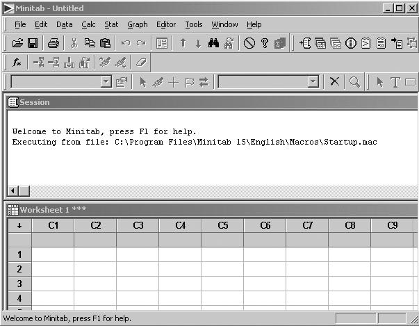
Figure 1shows you four important aspects of Minitab.The menu bar is where you choose commands.For instance,click on Stat and a pull-down menu appears that contains all of the statistical techniques available.The toolbar displays buttons for commonly used functions.Note that these buttons change depending on which Minitab window is open.There are two separate windows on the Minitab screen:the data window,where you enter,edit,and view the column data for each worksheet;and the session window,which displays text output,such as tables of statistics.
Specific instructions will be given to enable you to enter data into the Minitab spreadsheet and to activate forecasting procedures to produce needed forecasts.
FIGURE 1
Basic Minitab Screen
Introduction to Forecasting
Excel Applications
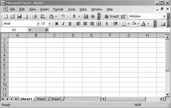
Excel is a popular spreadsheet program that is frequently used for forecasting.Figure 2 shows the opening screen of Version 2003.Data are entered in the rows and columns of the spreadsheet,and then commands are issued to perform various operations on the entered data.
For example,annual salaries for a number of employees could be entered into column A and the average of these values calculated by Excel.As another example, employee ages could be placed in column B and the relationship between age and salary examined.
There are several statistical functions available on Excel that may not be on the drop-down menus on your screen.To activate these functions,click on the following:
Tools>Add-Ins
The Add-Ins dialog box appears.Select Analysis ToolPak and click on OK. It is strongly recommended that an Excel add-in be used to help with the multitude of statistical computations required by the forecasting techniques discussed in thistext.
References
Bernstein,P.L. Against the Gods:The Remarkable Story of Risk. New York:Wiley,1996.
Carlberg,C.“Use Excel’s Forecasting to Get Terrific Projections.” Denver Business Journal 47 (18) (1996):2B.
Chase,C.W.,Jr.“Selecting the Appropriate Forecasting Method.” Journal of Business Forecasting 15 (Fall 1997):2.
Diebold,F.X. Elements of Forecasting,3rd ed. Cincinnati,Ohio:South-Western,2004.
FIGURE 2 Basic Excel Screen
Introduction to Forecasting
Georgoff,D.M.,and R.G.Mardick.“Manager’s Guide to Forecasting.” Harvard Business Review 1 (1986):110–120.
Hogarth,R.M.,and S.Makridakis.“Forecasting and Planning:An Evaluation.” Management Science 27 (2) (1981):115–138.
Hyndman,R.J.,and J.K.Ord,eds.“Special Issue: Twenty Five Years of Forecasting.” International Journal of Forecasting 22 (2006):413–636.
Levenbach,H.,and J.P.Cleary. Forecasting Practice and Process for Demand Management.Belmont, Calif.:Thomson Brooks/Cole,2006.
Makridakis,S.“The Art and Science of Forecasting.” International Journal of Forecasting 2 (1986):15–39.
Newbold,P.,and T.Bos. Introductory Business and Economic Forecasting,2nd ed.Cincinnati,Ohio: South-Western,1994. Ord,J.K.,and S.Lowe.“Automatic Forecasting.” American Statistician 50 (1996):88–94. Perry,S.“Applied Business Forecasting.” Management Accounting 72 (3) (1994):40. Pindyck,R.S.,and D.L.Rubinfeld. Econometric Models and Economic Forecasts,4th ed.New York:McGraw-Hill,1998. Wright,G.,and P.Ayton,eds. Judgemental Forecasting. New York:Wiley,1987.
This page intentionally left blank
EXPLORING DATA PATTERNS AND AN INTRODUCTION TO FORECASTING TECHNIQUES
One of the most time-consuming and difficult parts of forecasting is the collection of valid and reliable data.Data processing personnel are fond of using the expression “garbage in,garbage out”(GIGO).This expression also applies to forecasting.A forecast can be no more accurate than the data on which it is based.The most sophisticated forecasting model will fail if it is applied to unreliable data.
Modern computer power and capacity have led to an accumulation of an incredible amount of data on almost all subjects.The difficult task facing most forecasters is how to find relevant data that will help solve their specific decision-making problems.
Four criteria can be applied when determining whether data will be useful:
1.Data should be reliable and accurate.Proper care must be taken that data are collected from a reliable source with proper attention given to accuracy.
2.Data should be relevant.The data must be representative of the circumstances for which they are being used.
3.Data should be consistent.When definitions concerning data collection change, adjustments need to be made to retain consistency in historical patterns.This can be a problem,for example,when government agencies change the mix or “market basket”used in determining a cost-of-living index.Years ago personal computers were not part of the mix of products being purchased by consumers; now they are.
4.Data should be timely.Data collected,summarized,and published on a timely basis will be of greatest value to the forecaster.There can be too little data (not enough history on which to base future outcomes) or too much data (data from irrelevant historical periods far in the past).
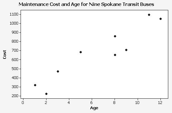
Generally,two types of data are of interest to the forecaster.The first is data collected at a single point in time,be it an hour,a day,a week,a month,or a quarter.The second is observations of data made over time.When all observations are fromthe same time period,we call them cross-sectional data.The objective is to examine such data and then to extrapolate or extend the revealed relationships to the larger population.Drawing a random sample of personnel files to study the circumstances of the employees of a company is one example.Gathering data on theage and current maintenance cost of nine Spokane Transit Authority buses isanother.A scatter diagram such as Figure 1helps us visualize the relationship and suggests age might be used to help in forecasting the annual maintenance budget.
Exploring Data Patterns and an Introduction to Forecasting Techniques
Cross-sectional data are observations collected at a single point in time.
Any variable that consists of data that are collected,recorded,or observed over successive increments of time is called a time series. Monthly U.S.beer production is an example of a time series.
A time series consists of data that are collected,recorded,or observed over successive increments of time.
EXPLORING TIME SERIES DATA PATTERNS
One of the most important steps in selecting an appropriate forecasting method for time series data is to consider the different types of data patterns.There are typically four general types of patterns:horizontal,trend,seasonal,and cyclical.
When data collected over time fluctuate around a constant level or mean,a horizontal pattern exists.This type of series is said to be stationary in its mean.Monthly sales for a food product that do not increase or decrease consistently over an extended period would be considered to have a horizontal pattern.
When data grow or decline over several time periods,a trend pattern exists.Figure 2 shows the long-term growth (trend) of a time series variable (such as housing costs) with data points one year apart.A linear trend line has been drawn to illustrate this growth.Although the variable housing costs have not increased every year,the movement of the variable has been generally upward between periods 1 and 20.Examples of the basic forces that affect and help explain the trend of a series are population growth, price inflation,technological change,consumer preferences,and productivity increases.
FIGURE 1 Scatter Diagram of Age and Maintenance Cost for Nine Spokane Transit Authority Buses
Exploring Data Patterns and an Introduction to Forecasting Techniques
Many macroeconomic variables,like the U.S.gross national product (GNP), employment,and industrial production exhibit trendlike behavior.Figure 10contains another example of a time series with a prevailing trend.This figure shows the growth of operating revenue for Sears from 1955 to 2004.
The trend is the long-term component that represents the growth or decline in the time series over an extended period of time.
When observations exhibit rises and falls that are not of a fixed period,a cyclical pattern exists.The cyclical component is the wavelike fluctuation around the trend that is usually affected by general economic conditions.A cyclical component,if it exists, typically completes one cycle over several years.Cyclical fluctuations are often influenced by changes in economic expansions and contractions,commonly referred to as the business cycle.Figure 2also shows a time series with a cyclical component.The cyclical peak at year 9 illustrates an economic expansion and the cyclical valley at year 12 an economic contraction.
The cyclical component is the wavelike fluctuation around the trend.
When observations are influenced by seasonal factors,a seasonal pattern exists. The seasonal component refers to a pattern of change that repeats itself year after year. For a monthly series,the seasonal component measures the variability of the series each January,each February,and so on.For a quarterly series,there are four seasonal elements,one for each quarter.Figure 3shows that electrical usage for Washington
FIGURE 2 Trend and Cyclical Components of an Annual Time Series Such as Housing Costs
Exploring Data Patterns and an Introduction to Forecasting Techniques
Electrical Usage for Washington Water Power: 1980–1991
Water Power residential customers is highest in the first quarter (winter months) of each year.Figure 14shows that the quarterly sales for Coastal Marine are typically low in the first quarter of each year.Seasonal variation may reflect weather conditions, school schedules,holidays,or length of calendar months.
The seasonal component is a pattern of change that repeats itself year after year.
EXPLORING DATA PATTERNS WITH AUTOCORRELATION ANALYSIS
When a variable is measured over time,observations in different time periods are frequently related or correlated.This correlation is measured using the autocorrelation coefficient.
Autocorrelation is the correlation between a variable lagged one or more time periods and itself.
Data patterns,including components such as trend and seasonality,can be studied using autocorrelations.The patterns can be identified by examining the autocorrelation coefficients at different time lags of a variable.
The concept of autocorrelation is illustrated by the data presented in Table 1.Note that variables are actually the Y values that have been lagged by one and two time periods,respectively.The values for March,which are shown on the row for time period 3,are March sales,;February sales,;and January sales, Y t - 2 = 123 Y t - 1 = 130 Y t = 125 Y t - 1 and Y t - 2
FIGURE 3 Electrical Usage for Washington Water Power Company, 1980–1991
Exploring Data Patterns and an Introduction to Forecasting Techniques
TABLE
1 VCR Data for Example 1
Equation 1 is the formula for computing the lag k autocorrelation coefficient (rk) between observations, Yt and that are k periods apart.
where
rk = the autocorrelation coefficient for a lag of k periods
Y = the mean of the values of the series
Y t = the observation in time period t
Y t - k = the observation k time periods earlier or at time period t - k
Example 1
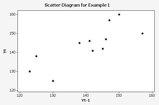
Harry Vernon has collected data on the number of VCRs sold last year by Vernon’s Music Store.The data are presented in Table 1.Table 2shows the computations that lead to the calculation of the lag 1 autocorrelation coefficient.Figure 4contains a scatter diagram of the pairs of observations ().It is clear from the scatter diagram that the lag 1 correlation will be positive.
The lag 1 autocorrelation coefficient (r1),or the autocorrelation between Yt and , is computed using the totals from Table 2and Equation 1.Thus,
As suggested by the plot in Figure 4,positive lag 1 autocorrelation exists in this time series.The correlation between Yt and or the autocorrelation for time lag 1,is .572.This means that the successive monthly sales of VCRs are somewhat correlated with each other. This information may give Harry valuable insights about his time series,may help him prepare to use an advanced forecasting method,and may warn him about using regression analysis with his data.
Exploring Data Patterns and an Introduction to Forecasting Techniques
TABLE 2 Computation of the Lag 1 Autocorrelation Coefficient for the Data in Table 1
The second-order autocorrelation coefficient (r2),or the correlation between Yt and for Harry’s data,is also computed using Equation 1.
FIGURE 4 Scatter Diagram for Vernon’s Music Store Data for Example 1
Exploring Data Patterns and an Introduction to Forecasting Techniques
It appears that moderate autocorrelation exists in this time series lagged two time periods.The correlation between Yt and ,or the autocorrelation for time lag 2,is .463.Notice that the autocorrelation coefficient at time lag 2 (.463) is less than the autocorrelation coefficient at time lag 1 (.572).Generally,as the number of time lags (k) increases,the magnitudes of the autocorrelation coefficients decrease.
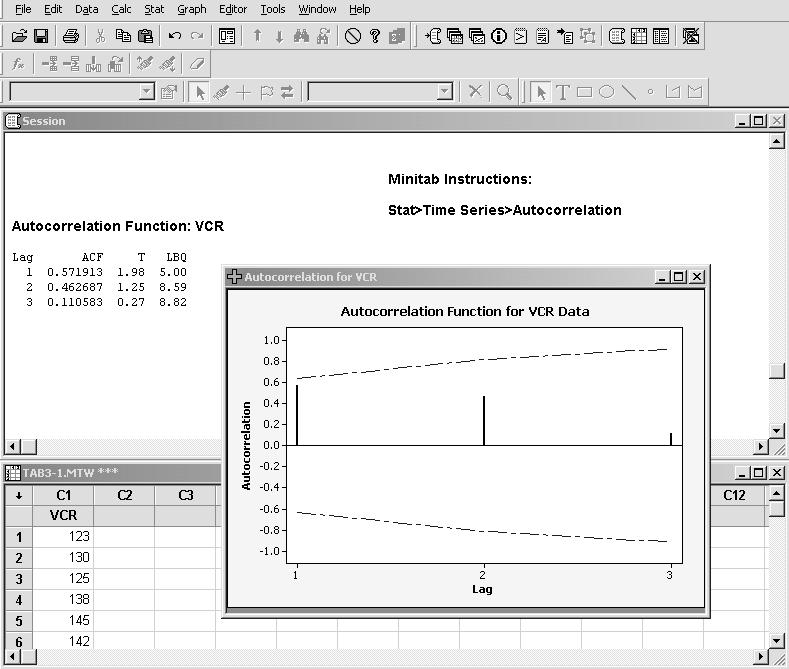
Figure 5shows a plot of the autocorrelations versus time lags for the Harry Vernon data used in Example 1.The horizontal scale on the bottom of the graph shows each time lag of interest:1,2,3,and so on.The vertical scale on the left shows the possible range of an autocorrelation coefficient, -1 to 1.The horizontal line in the middle of the graph represents autocorrelations of zero.The vertical line that extends upward above time lag 1 shows an autocorrelation coefficient of .57,or .The vertical line that extends upward above time lag 2 shows an autocorrelation coefficient of .46,or .The dotted lines and the T (test) and LBQ (Ljung-Box Q) statistics displayed in the Session window will be discussed in Examples 2 and 3.Patterns in a correlogram are used to analyze key features of the data,a concept demonstrated in the next section.The Minitab computer package (see the Minitab Applications section at the end of the chapter for specific instructions) can be used to compute autocorrelations and develop correlograms.
The correlogram or autocorrelation function is a graph of the autocorrelations for various lags of a time series.
FIGURE 5 Correlogram or Autocorrelation Function for the Data Used in Example 1
Exploring Data Patterns and an Introduction to Forecasting Techniques
With a display such as that in Figure 5,the data patterns,including trend and seasonality,can be studied.Autocorrelation coefficients for different time lags for a variable can be used to answer the following questions about a time series:
1.Are the data random?
2.Do the data have a trend (are they nonstationary)?
3.Are the data stationary?
4.Are the data seasonal?
If a series is random,the autocorrelations between Yt and for any time lag k are close to zero.The successive values of a time series are not related to each other.
If a series has a trend,successive observations are highly correlated,and the autocorrelation coefficients typically are significantly different from zero for the first several time lags and then gradually drop toward zero as the number of lags increases. The autocorrelation coefficient for time lag 1 will often be very large (close to 1).The autocorrelation coefficient for time lag 2 will also be large.However,it will not be as large as for time lag 1.
If a series has a seasonal pattern,a significant autocorrelation coefficient will occur at the seasonal time lag or multiples of the seasonal lag.The seasonal lag is 4 for quarterly data and 12 for monthly data.
How does an analyst determine whether an autocorrelation coefficient is significantly different from zero for the data of Table 1? Quenouille (1949) and others have demonstrated that the autocorrelation coefficients of random data have a sampling distribution that can be approximated by a normal curve with a mean of zero and an approximate standard deviation of . Knowing this,the analyst can compare the sample autocorrelation coefficients with this theoretical sampling distribution and determine whether,for given time lags,they come from a population whose mean is zero.
Actually,some software packages use a slightly different formula,as shown in Equation 2,to compute the standard deviations (or standard errors) of the autocorrelation coefficients.This formula assumes that any autocorrelation before time lag k is different from zero and any autocorrelation at time lags greater than or equal to k is zero.For an autocorrelation at time lag 1,the standard error is used. (2)
where
ri = the autocorrelation at time lag i of the autocorrelation at time lag k
k = the time lag
n = the number of observations in the time series
This computation will be demonstrated in Example 2.If the series is truly random, almost all of the sample autocorrelation coefficients should lie within a range specified by zero,plus or minus a certain number of standard errors.At a specified confidence level,a series can be considered random if each of the calculated autocorrelation coefficients is within the interval about 0 given by 0 ± t × SE(rk),where the multiplier t is an appropriate percentage point of a t distribution.
Exploring Data Patterns and an Introduction to Forecasting Techniques
Although testing each rk to see if it is individually significantly different from 0 is useful,it is also good practice to examine a set of consecutive rk’s as a group.We can use a portmanteau test to see whether the set,say,of the first 10 rk values,is significantly different from a set in which all 10 values are zero.
One common portmanteau test is based on the Ljung-Box Q statistic (Equation 3).This test is usually applied to the residuals of a forecast model.If the autocorrelations are computed from a random (white noise) process,the statistic Q has a chisquare distribution with m (the number of time lags to be tested) degrees of freedom.For the residuals of a forecast model,however,the statistic Q has a chi-square distribution with the degrees of freedom equal to m minus the number of parameters estimated in the model.The value of the Q statistic can be compared with the chi-square table (Table 4 in Appendix:Tables) to determine if it is larger than we would expect it to be under the null hypothesis that all the autocorrelations in the set are zero.Alternatively,the p -value generated by the test statistic Q can be computed and interpreted.The Q statistic is given in Equation 3.It will be demonstrated in Example 3.
(3) where
n = the number of observations in the time series
k = the time lag
m = the number of time lags to be tested
rk = the sample autocorrelation function of the residuals lagged k time periods
Are the Data Random?
A simple random model,often called a white noise model, is displayed in Equation 4. Observation Yt is composed of two parts: c, the overall level,and t,which is the random error component.It is important to note that the t component is assumed to be uncorrelated from period to period.
(4)
Are the data in Table 1consistent with this model? This issue will be explored in Examples 2 and 3.
Example 2
A hypothesis test is developed to determine whether a particular autocorrelation coefficient is significantly different from zero for the correlogram shown in Figure 5.The null and alternative hypotheses for testing the significance of the lag 1 population autocorrelation coefficient are
If the null hypothesis is true,the test statistic
(5)
Exploring Data Patterns and an Introduction to Forecasting Techniques
has a t distribution with .Here,,so for a 5% significance level,the decision rule is as follows:
If t 2.2 or t 2.2,reject H0 and conclude the lag 1 autocorrelation is significantly different from 0.
The critical values 2.2 are the upper and lower .025 points of a t distribution with 11 degrees of freedom.The standard error of r1 is ,and the value of the test statistic becomes
Using the decision rule above,cannot be rejected,since - 2.2 < 1.98 < 2.2. Notice the value of our test statistic,,is the same as the quantity in the Lag 1 row under the heading T in the Minitab output in Figure 5.The T values in the Minitab output are simply the values of the test statistic for testing for zero autocorrelation at the various lags.
To test for zero autocorrelation at time lag 2,we consider
and the test statistic
Using Equation 2,
and
This result agrees with the T value for Lag 2 in the Minitab output in Figure 5. Using the decision rule above,cannot be rejected at the .05 level,since -2.2 1.25 2.2.An alternative way to check for significant autocorrelation is to construct, say,95% confidence limits centered at 0.These limits for time lags 1 and 2 are as follows:
Autocorrelation significantly different from 0 is indicated whenever a value for rk falls outside the corresponding confidence limits.The 95% confidence limits are shown in Figure 5by the dashed lines in the graphical display of the autocorrelation function.
Example 3
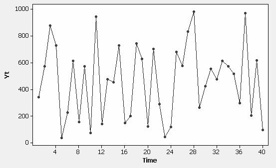
Minitab was used to generate the time series of 40 pseudo-random three-digit numbers shown in Table 3.Figure 6shows a time series graph of these data.Because these data are random (independent of one another and all from the same population),autocorrelations for
Exploring Data Patterns and an Introduction to Forecasting Techniques
all time lags should theoretically be equal to zero.Of course,the 40 values in Table 3are only one set of a large number of possible samples of size 40.Each sample will produce different autocorrelations.Most of these samples will produce sample autocorrelation coefficients that are close to zero.However,it is possible that a sample will produce an autocorrelation coefficient that is significantly different from zero just by chance.
Next,the autocorrelation function shown in Figure 7is constructed using Minitab.Note that the two dashed lines show the 95% confidence limits.Ten time lags are examined,and all the individual autocorrelation coefficients lie within these limits.There is no reason to doubt that each of the autocorrelations for the first 10 lags is zero.However,even though the individual sample autocorrelations are not significantly different from zero,are the magnitudes of the first 10 rk’s as a group larger than one would expect under the hypothesis of no autocorrelation at any lag? This question is answered by the Ljung-Box Q (LBQ in Minitab) statistic.
If there is no autocorrelation at any lag,the Q statistic has a chi-square distribution with,in this case,.Consequently,a large value for Q (in the tail of the chi-square distribution) is evidence against the null hypothesis.From Figure 7,the value of Q (LBQ) for 10 time lags is 7.75.From Table 4in Appendix:Tables,the upper .05 point of a chi-square distribution with 10 degrees of freedom is 18.31.Since 7.75 < 18.31,the null hypothesis cannot be rejected at the 5% significance level.These data are uncorrelated at any time lag,a result consistent with the model in Equation 4. df = 10
TABLE 3 Time Series of 40 Random Numbers for Example 3
FIGURE 6 Time Series Plot of 40 Random Numbers Used in Example 3