13.5 Summary and References Problems 14 Power Spectrum Estimation
14.1 Estimation of Spectra from Finite-Duration Observations of Signals
14.1.1 Computation of the Energy Density Spectrum
14.1.2 Estimation of the Autocorrelation and Power Spectrum of Random 966 Signals: The Periodogram
14.1.3 The Use of the OFT in Power Spectrum Estimation 971 14.2 Nonparametric Methods for Power Spectrum Estimation
The Blackman and Tukey Method: Smoothing the Periodogram
Performance Characteristics of Nonparametric Power Spectrum
Estimators 14.2.5 Computational Requirements of Nonparametric Power Spectrum
14.3.1 Relationships Between the Autocorrelation and the Model
14.3.2 The Yule-Walker Method for the AR Model Parameters
14.3.3 The Burg Method for the AR Model Parameters
14.3.4 Unconstrained Least-Squares Method for the AR Model
Parameters
14.3.5 Sequential Estimation Methods for the AR Model Parameters
14.3.6 Selection of AR Model Order 996
14.3.7 MA Model for Power Spectrum Estimation
14.3.8 ARMA Model for Power Spectrum Estimation
Preface
This book was developed based on our teaching of undergraduate- and graduatelevel courses in digital signal processing over the past several years. In this book we present the fundamentals of discrete-time signals, systems, and modern digital processing as well as applications for students in electrical engineering, computer engineering, and computer science. The book is suitable for either a one-semester or a two-semester undergraduate-level course in discrete systems and digital signal processing. It is also intended for use in a one-semester first-year graduate-level course in digital signal processing.
It is assumed that the student has had undergraduate courses in advanced calculus (including ordinary differential equations) and linear systems for continuous-time signals, including an introduction to the Laplace transform. Although the Fourier series and Fourier transforms of periodic and aperiodic signals are described in Chapter 4, we expect that many students may have had this material in a prior course.
Balanced coverage of both theory and practical applications is provided. A large number of well-designed problems are provided to help the student in mastering the subject matter. A solutions manual is available for download for instructors only. Additionally, Microsoft PowerPoint slides of text figures are available for instructors on the publisher'S website.
In the fourth edition of the book, we have added a new chapter on adaptive filters and have substantially modified and updated the chapters on muItirate digital signal processing and on sampling and reconstruction of signals. We have also added new material on the discrete cosine transform.
In Chapter 1 we describe the operations involved in the analog-to-digital conversion of analog signals. The process of sampling a sinusoid is described in some detail and the problem of aliasing is explained. Signal quantization and digital-toanalog conversion are also described in general terms, but the analysis is presented in subsequent chapters.
Chapter 2 is devoted entirely to the characterization and analysis of linear timeinvariant (shift-invariant) discrete-time systems and discrete-time signals in the time domain. The convolution sum is derived and systems are categorized according to the duration of their impulse response as a finite-duration impulse response (FIR) and as an infinite-duration impulse response (IIR). Linear time-invariant systems characterized by difference equations are presented and the solution of difference equations with initial conditions is obtained. The chapter concludes with a treatment of discrete-time correlation.
The z-transform is introduced in Chapter 3. Both the bilateral and the unilateral z-transforms are presented, and methods for determining the inverse z-transform are described. Use of the z-transform in the analysis of linear time-invariant systems is illustrated, and important properties of systems, such as causality and stability, are related to z-domain characteristics.
Chapter 4 treats the analysis of signals in the frequency domain. Fourier series and the Fourier transform are presented for both continuous-time and discrete-time signals.
In Chapter 5, linear time-invariant (LTl) discrete systems are characterized in the frequency domain by their frequency response function and their response to periodic and aperiodic signals is determined. A number of important types of discrete-time systems are described, including resonators, notch filters, comb filters, all-pass filters, and oscillators. The design of anum ber of simple FIR and IIR filters is also considered In addition, the student is introduced to the concepts of minimum-phase, mixedphase, and maximum-phase systems and to the problem of deconvolution.
Chapter 6 provides a thorough treatment of sampling of continuous-time signals and the reconstruction of the signals from their samples. Our coverage includes the sampling and reconstruction of bandpass signals, the sampling of discrete-time signals, and AID and DI A conversion. The chapter concludes with the treatment of oversampling AID and D/A converters.
The DFf, its properties and its applications, are the topics covered in Chapter 7. Two methods are described for using the DFf to perform linear filtering. The use of the DFf to perform frequency analysis of signals is also described. The final topic treated in this chapter is the discrete cosine transform.
Chapter 8 covers the efficient computation of the OFT. Included in this chapter are descriptions of radix-2, radix-4, and split-radix fast Fourier transform (FFT) algorithms, and applications of the FFTalgorithms to the computation of convolution and correlation. The Goertzel algorithm and the chirp-z transform are introduced as two methods for computing the DFf using linear filtering.
Chapter 9 treats the realization of IIR and FIR systems. This treatment includes direct-form, cascade, parallel, lattice, and lattice-Iadderrealizations. The chapter also examines quantization effects in a digital implementation of FIR and IIR systems.
Techniques for design of digital FIR and IIR filters are presented in Chapter 10. The design techniques include both direct methods in discrete time and methods involving the conversion of analog filters into digital filters by various transformations.
Chapter 11 treats sampling-rate conversion and its applications to multirate digital signal processing. In addition to describing decimation and interpolation by integer and rational factors, we describe methods for sampling-rate conversion by an arbitrary factor and implementations by polyphase filter structures. This chapter also treats digital filter banks, two-channel quadrature mirror filters (QMF) and M-channel QMF banks.
Linear prediction and optimum linear (Wiener) filters are treated in Chapter 12. Also included in this chapter are descriptions of the Levinson-Durbin algorithm and Schur algorithm for solving the normal equations, as well as the AR lattice and ARMA lattice-ladder filters.
Preface xix
Chapter 13 treats single-channel adaptive filters based on the LMS algorithm and on recursive least squares (RLS) algorithms. Both direct form FIR and lattice RLS algorithms and filter structures are described.
Power spectrum estimation is the main topic of Chapter 14. Our coverage includes a description of non parametric and model-based (parametric) methods. Also described are eigen-decomposition-based methods, including MUSIC and ESPRIT.
A one-semester senior-level course for students who have had prior exposure to discrete systems can use the material in Chapters 1 through 5 for a quick review and then proceed to cover Chapters 6 through 10.
In a first-year graduate-level course in digital signal processing, the first six chapters provide the student with a good review of discrete-time systems. The instructor can move quickly through most of this material and then cover Chapters 7 through 11, followed by selected topics from Chapters 12 through 14.
Many examples throughout the book and approximately 500 homework problems are included throughout the book. Answers to selected problems appear in the back of the book. Many of the homework problems can be solved numerically on a computer, using a software package such as MATLAB®. Available for use as a selfstudy companion to the textbook is a student manual: Student Manual for Digital Signal Processing with MATLAB®. MATLAB is incorporated as the basic software tool for this manual. The instructor may also wish to consider the use of other supplementary books that contain computer-based exercises, such as Computer-Based Exercisesfor Signal Processing Using MATLAB (Prentice Hall, 1994) by C. S. Burrus et at.
The authors are indebted to their many faculty colleagues who have provided valuable suggestions through reviews of previous editions of this book. These include W. E. Alexander, G. Arslan, Y. Bresler, I Deller, F. DePiero, V. Ingle, IS. Kang, C. Keller, H. Lev-Ari, L. Merakos, W. Mikhael, P. Monticciolo, C. Nikias, M. Schetzen, E. Serpedin, T. M. Sullivan, H. Trussell, S. Wilson, and M. Zoltowski. We are also indebted to R. Price for recommending the inclusion of split-radix FFT algorithms and related suggestions. Finally, we wish to acknowledge the suggestions and comments of many former graduate students, and especially those by A. L. Kok, I Lin, E. Sozer, and S. Srinidhi, who assisted in the preparation of several illustrations and the solutions manual.
JOHN G. PROAKIS DIMITRIS G. MANOLAKIS
CHAPTER
Introduction
Digital signal processing is an area of science and engineering that has developed rapidly over the past 40 years. This rapid development is a result of the significant advances in digital computer technology and integrated-circuit fabrication. The digital computers and associated digital hardware of four decades ago were relatively large and expensive and, as a consequence, their use was limited to general-purpose non-real-time (off-line) scientific computations and business applications. The rapid developments in integrated-circuit technology, starting with medium-scale integration (MSI) and progressing to large-scale integration (LSI), and now, very-large-scale integration (VLSI) of electronic circuits has spurred the development of powerful, smaller, faster, and cheaper digital computers and special-purpose digital hardware. These inexpensive and relatively fast digital circuits have made it possible to construct highly sophisticated digital systems capable of performing complex digital signal processing functions and tasks, which are usually too difficult and/or too expensive to be performed by analog circuitry or analog signal processing systems. Hence many of the signal processing tasks that were conventionally performed by analog means are realized today by less expensive and often more reliable digital hardware.
We do not wish to imply that digital signal processing is the proper solution for all signal processing problems. Indeed, for many signals with extremely wide bandwidths, real-time processing is a requirement. For such signals, analog or, perhaps, optical signal processing is the only possible solution. However, where digital circuits are available and have sufficient speed to perform the signal processing, they are usually preferable.
Not only do digital circuits yield cheaper and more reliable systems for signal processing, they have other advantages as well. In particular, digital processing hardware allows programmable operations. Through software, one can more eas-
Chapter I Introduction
ily modify the signal processing functions to be performed by the hardware. Thus digital hardware and associated software provide a greater degree of flexibility in system design. Also, there is often a higher order of precision achievable with digital hardware and software compared with analog circuits and analog signal processing systems. For all these reasons, there has been an explosive growth in digital signal processing theory and applications over the past three decades.
In this book our objective is to present an introduction of the basic analysis tools and techniques for digital processing of signals. We begin by introducing some of the necessary terminology and by describing the important operations associated with the process of converting an analog signal to digital form suitable for digital processing. As we shall see, digital processing of analog signals has some drawbacks. First, and foremost, conversion of an analog signal to digital form, accomplished by sampling the signal and quantizing the samples, results in a distortion that prevents us from reconstructing the original analog signal from the quantized samples. Control of the amount of this distortion is achieved by proper choice of the sampling rate and the precision in the quantization process. Second, there are finite precision effects that must be considered in the digital processing of the quantized samples. While these important issues are considered in some detail in this book, the emphasis is on the analysis and design of digital signal processing systems and computational techniques.
1.1 Signals, Systems, and Signal Processing
A signal is defined as any physical quantity that varies with time, space, or any other independent variable or variables. Mathematically, we describe a signal as a function of one or more independent variables. For example, the functions
sl(t)=5t
S2(t) = 20t 2
(1.1.1)
describe two signals, one that varies linearly with the independent variable t (time) and a second that varies quadratically with t. As another example, consider the function
sex. y) = 3x + 2xy + wi ( 1.1.2)
This function describes a signal of two independent variables x and y that could represent the two spatial coordinates in a plane.
The signals described by (1.1.1) and (1.1.2) belong to a class of signals that are precisely defined by specifying the functional dependence on the independent variable. However, there are cases where such a functional relationship is unknown or too highly complicated to be of any practical use.
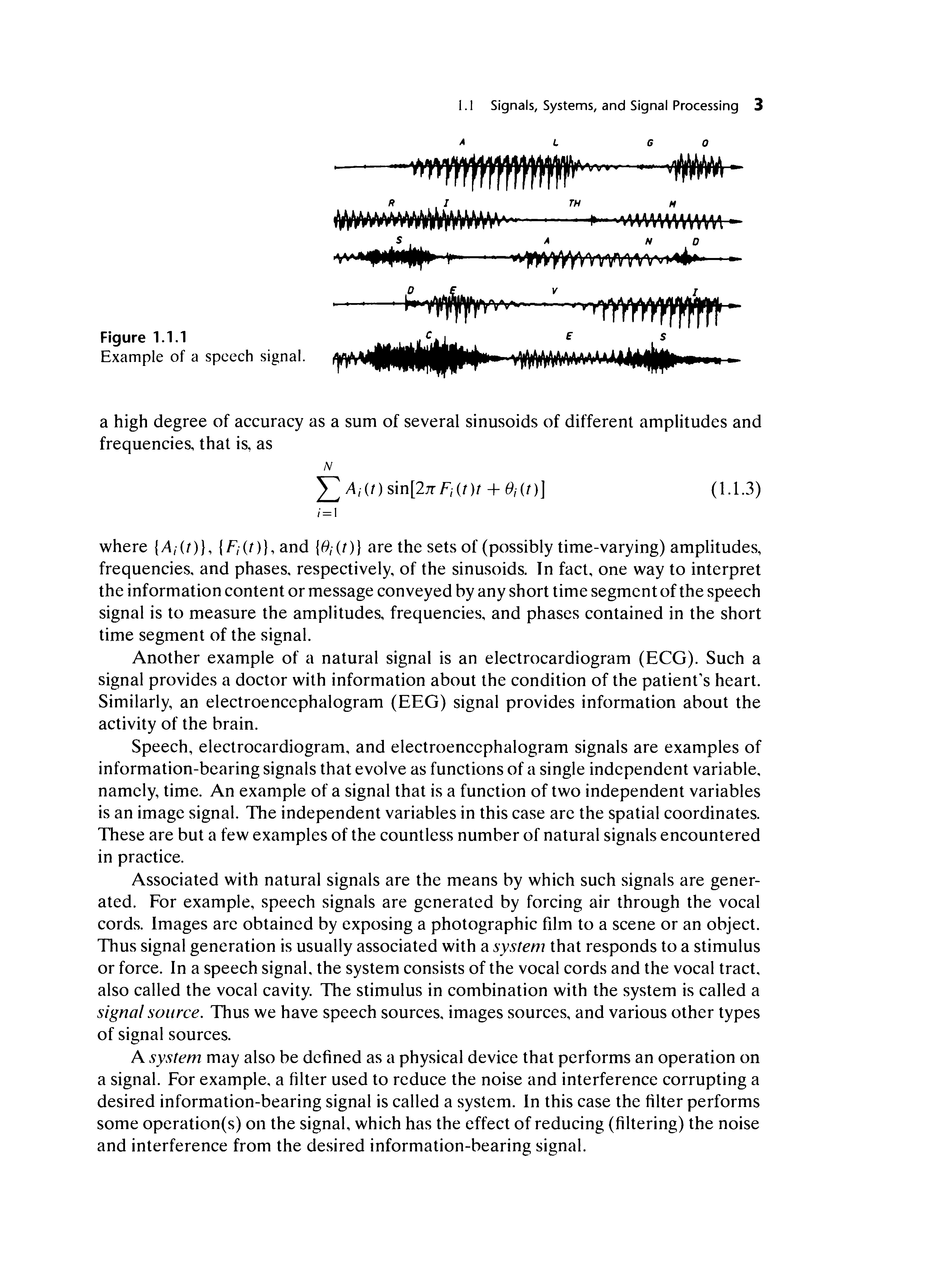
For example, a speech signal (see Fig. 1.1.1) cannot be described functionally by expressions such as (1.1.1). In general, a segment of speech may be represented to
Figure 1.1.1
Example of a spcech signal.
a high degree of accuracy as a sum of several sinusoids of different amplitudes and frequencies.. that is.. as
where (A;(t)), (F;(t»), and lei (t) I are the sets of (possibly time-varying) amplitudes, frequencies. and phases. respectively. of the sinusoids. In fact, one way to interpret the information content or message conveyed by any short time segment of the speech signal is to measure the amplitudes, frequencies. and phases contained in the short time segment of the signal.
Another example of a natural signal is an electrocardiogram (ECG). Such a signal provides a doctor with information about the condition of the patient's heart. Similarly, an electroencephalogram (EEG) signal provides information about the activity of the brain.
Speech, electrocardiogram, and electroencephalogram signals are examples of information-bearing signals that evolve as functions of a single independent variable. namely, time. An example of a signal that is a function of two independent variables is an image signal. The independent variables in this case are the spatial coordinates. These are but a few examples of the countless number of natural signals encountered in practice.
Associated with natural signals are the means by which such signals are generated. For example, speech signals are generated by forcing air through the vocal cords. Images are obtained by exposing a photographic film to a scene or an object. Thus signal generation is usually associated with a system that responds to a stimulus or force. In a speech signaL the system consists of the vocal cords and the vocal tract. also called the vocal cavity. The stimulus in combination with the system is called a signal sOllrce. Thus we have speech sources. images sources, and various other types of signal sources.
A system may also be defined as a physical device that performs an operation on a signal. For example. a filter used to reduce the noise and interference corrupting a desired information-bearing signal is called a system. In this case the filter performs some operation(s) on the signal, which has the effect of reducing (filtering) the noise and interference from the desired information-bearing signal.
When we pass a signal through a system, as in filtering, we say that we have processed the signal. In this case the processing of the signal involves filtering the noise and interference from the desired signal. In general, the system is characterized by the type of operation that it performs on the signal. For example, if the operation is linear. the system is called linear. If the operation on the signal is nonlinear, the system is said to be nonlinear. and so forth. Such operations are usually referred to as signal processing.
For our purposes, it is convenient to broaden the definition of a system to include not only physical devices, but also software realizations of operations on a signal. In digital processing of signals on a digital computer. the operations performed on a signal consist of a number of mathematical operations as specified by a software program. In this case, the program represents an implementation of the system in software. Thus we have a system that is realized on a digital computer by means of a sequence of mathematical operations; that is, we have a digital signal processing system realized in software. For example. a digital computer can be programmed to perform digital filtering. Alternatively. the digital processing on the signal may be performed by digital hardware (logic circuits) configured to perform the desired specificd opcrations. In such a realization. we have a physical dcvice that performs the specified operations. In a broader sense. a digital system can bc implemented as a combination of digital hardware and software. each of which performs its own sct of specified operations.
This book deals with the processing of signals by digital means, either in software or in hardware. Since many of the signals encountered in practicc are analog, we will also consider the problem of converting an analog signal into a digital signal for processing. Thus we will be dealing primarily with digital systems. The operations performed by such a system can usually be specified mathematically. The method or set of rules for implementing the system by a program that performs the corresponding mathematical operations is called an algorithm. Usually. there are many ways or algorithms by which a system can be implemented, either in software or in hardware, to perform the desired operations and computations. In practice. we have an interest in devising algorithms that are computationally efficient, fast, and easily implemented. Thus a major topic in our study of digital signal processing is the discussion of efficicnt algorithms for performing such operations as filtering. correlation, and spectral analysis.
1.1 .1 Basic Elements of a Digital Signal Processing System
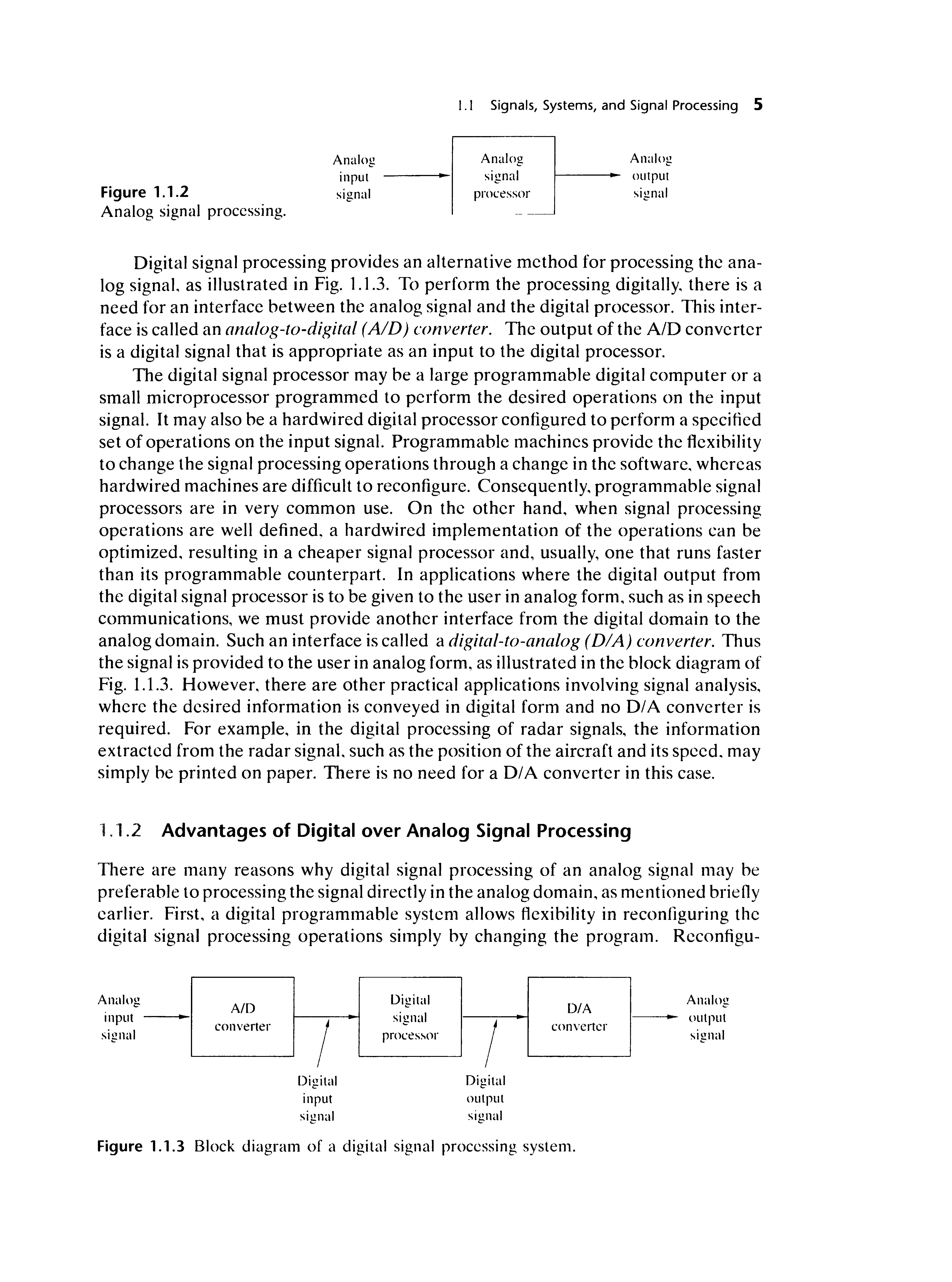
Most of the signals encountered in science and cngineering are analog in nature. That is, the signals are functions of a continuous variable, such as time or space. and usually take on values in a continuous range. Such signals may be processed directly by appropriate analog systems (such as filters, frequency analyzers. or frcquency multipliers) for the purpose of changing their characteristics or extracting some desired information. In such a case we say that the signal has been processed directly in its analog form. as illustrated in Fig. 1.1.2. Both the input signal and the output signal arc in analog form.
Figure 1.1.2
Analog signal processing.
Analog input ----I signal
1.1 Signals, Systems, and Signal Processing 5
Analog signal processor
Analog 1---- output signal
Digital signal processing provides an alternative method for processing the analog signal. as illustrated in Fig. 1.1.3. To perform the processing digitally. there is a need for an interface between the analog signal and the digital processor. This interface is called an analog-to-digital (AID) converter. The output of the AID converter is a digital signal that is appropriate as an input to the digital processor.
The digital signal processor may be a large programmable digital computer or a small microprocessor programmed to perform the desired operations on the input signal. It may also be a hardwired digital processor configured to perform a specified set of operations on the input signal. Programmable machines provide the flexibility to change the signal processing operations through a change in the software. whereas hardwired machines are difficult to reconfigure. Consequently. programmable signal processors are in very common use. On the other hand. when signal processing operations are well defined. a hardwired implementation of the operations can be optimized. resulting in a cheaper signal processor and, usually, one that runs faster than its programmable counterpart. In applications where the digital output from the digital signal processor is to be given to the user in analog form, such as in speech communications, we must provide another interface from the digital domain to the analog domain. Such an interface is called a digital-to-analog (DIA) converter. Thus the signal is provided to the user in analog form, as illustrated in the block diagram of Fig. 1.1.3. However. there are other practical applications involving signal analysis, where the desired information is conveyed in digital form and no D/A converter is required. For example, in the digital processing of radar signals, the information extracted from the radar signal. such as the position of the aircraft and its speed. may simply be printed on paper. There is no need for a D/A converter in this case.
1.1.2 Advantages of Digital over Analog Signal Processing
There are many reasons why digital signal processing of an analog signal may be preferable to processing the signal directly in the analog domain, as mentioned briefly earlier. First, a digital programmable system allows flexibility in reconJlguring the digital signal processing operations simply by changing the program. Reconfigu-
Figure 1.1.3 Block diagram of a digital signal processing system.
Chapter 1 Introduction
ration of an analog system usually implies a redesign of the hardware followed by testing and verification to see that it operates properly.
Accuracy considerations also play an important role in determining the form of the signal processor. Tolerances in analog circuit components make it extremely difficult for the system designer to control the accuracy of an analog signal processing system. On the other hand, a digital system provides much better control of accuracy requirements. Such requirements, in turn, result in specifying the accuracy requirements in the AID converter and the digital signal processor, in terms of word length, floating-point versus fixed-point arithmetic, and similar factors.
Digital signals are easily stored on magnetic media (tape or disk) without deterioration or loss of signal fidelity beyond that introduced in the AID conversion. As a consequence, the signals become transportable and can be processed off-line in a remote laboratory. The digital signal processing method also allows for the implementation of more sophisticated signal processing algorithms. It is usually very difficult to perform precise mathematical operations on signals in analog form but these same operations can be routinely implemented on a digital computer using software.
In some cases a digital implementation of the signal processing system is cheaper than its analog counterpart. The lower cost may be due to the fact that the digital hardware is cheaper, or perhaps it is a result of the flexibility for modifications provided by the digital implementation.
As a consequence of these advantages, digital signal processing has been applied in practical systems covering a broad range of disciplines. We cite, for example, the application of digital signal processing techniques in speech processing and signal transmission on telephone channels, in image processing and transmission, in seismology and geophysics, in oil exploration, in the detection of nuclear explosions, in the processing of signals received from outer space, and in a vast variety of other applications. Some of these applications are cited in subsequent chapters.
As already indicated, however, digital implementation has its limitations. One practical limitation is the speed of operation of AID converters and digital signal processors. We shall see that signals having extremely wide bandwidths require fast-sampling-rate AID converters and fast digital signal processors. Hence there are analog signals with large bandwidths for which a digital processing approach is beyond the state of the art of digital hardware.
1.2 Classification of Signals
The methods we use in processing a signal or in analyzing the response of a system to a signal depend heavily on the characteristic attributes of the specific signal. There are techniques that apply only to specific families of signals. Consequently, any investigation in signal processing should start with a classification of the signals involved in the specific application.
1.2.1 Multichannel and Multidimensional Signals
As explained in Section 1.1, a signal is described by a function of one or more independent variables. The value of the function (i.e., the dependent variable) can be
1.2 Classification of Signals 7 a real-valued scalar quantity, a complex-valued quantity, or perhaps a vector. For example, the signal
sl (t) = A sin 3;rrt is a real-valued signal. However, the signal
S2(t) = Ae j3JTt = A cos 3;rrt + j A sin 3;rrt is complex valued.
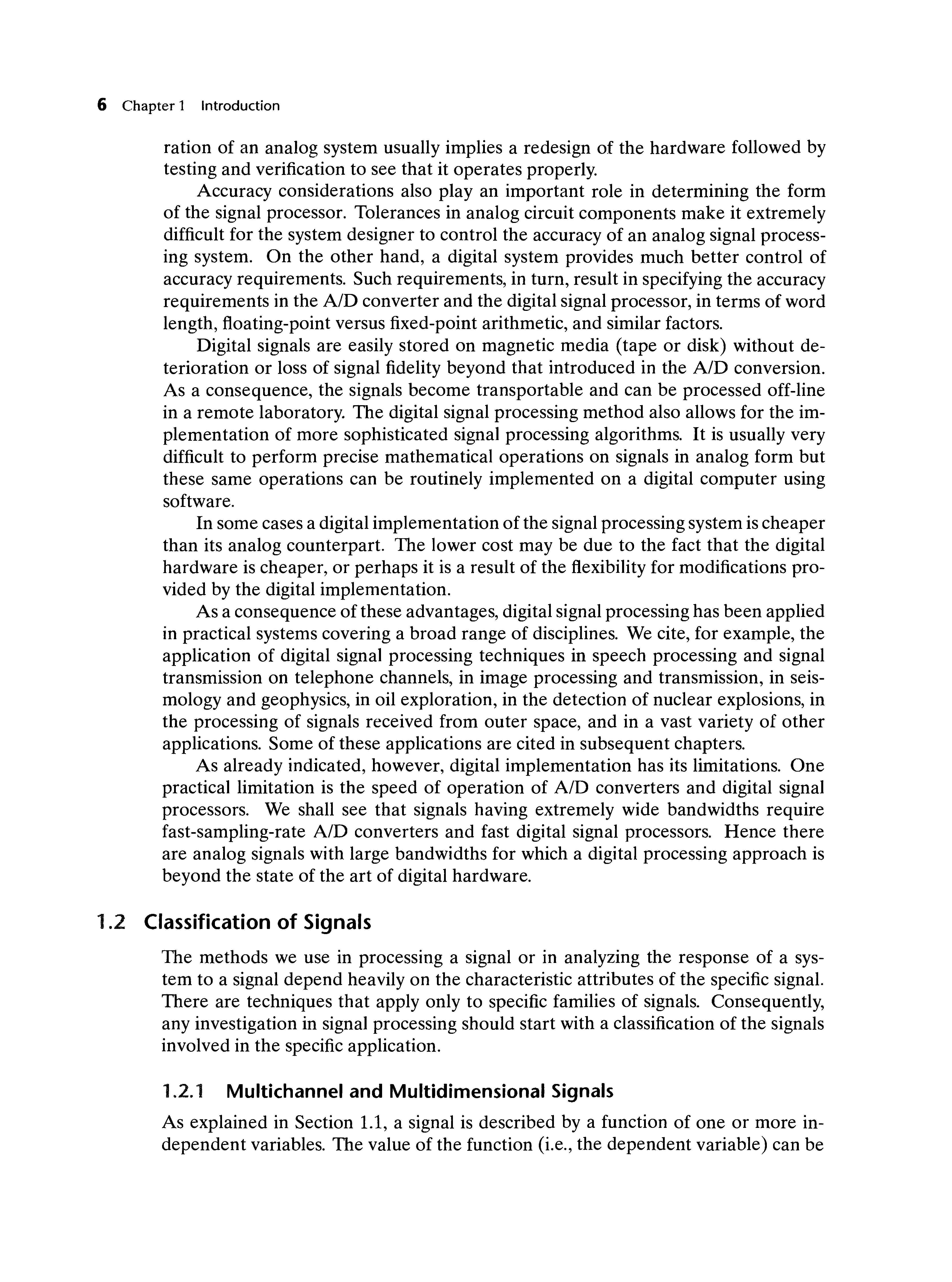
In some applications, signals are generated by multiple sources or multiple sensors. Such signals, in turn, can be represented in vector form. Figure 1.2.1 shows the three components of a vector signal that represents the ground acceleration due to an earthquake. This acceleration is the result of three basic types of elastic waves. The primary (P) waves and the secondary (S) waves propagate within the body of
rock and are longitudinal and transversal, respectively. The third type of elastic wave is called the surface wave, because it propagates near the ground surface. If sdl), k = 1,2, 3, denotes the electrical signal from the kth sensor as a function of time. the set of p = 3 signals can be represented by a vector S](I), where
We refer to such a vector of signals as a multichannel signal.In electrocardiography. for example, 3-lead and 12-lead electrocardiograms (ECG) are often used in practice, which result in 3-channel and 12-channel signals.
Let us now turn our attention to the independent variable(s). If the signal is a function of a single independent variable, the signal is called a one-dimensional signal. On the other hand, a signal is called M -dimensional if its value is a function of M independent variables.
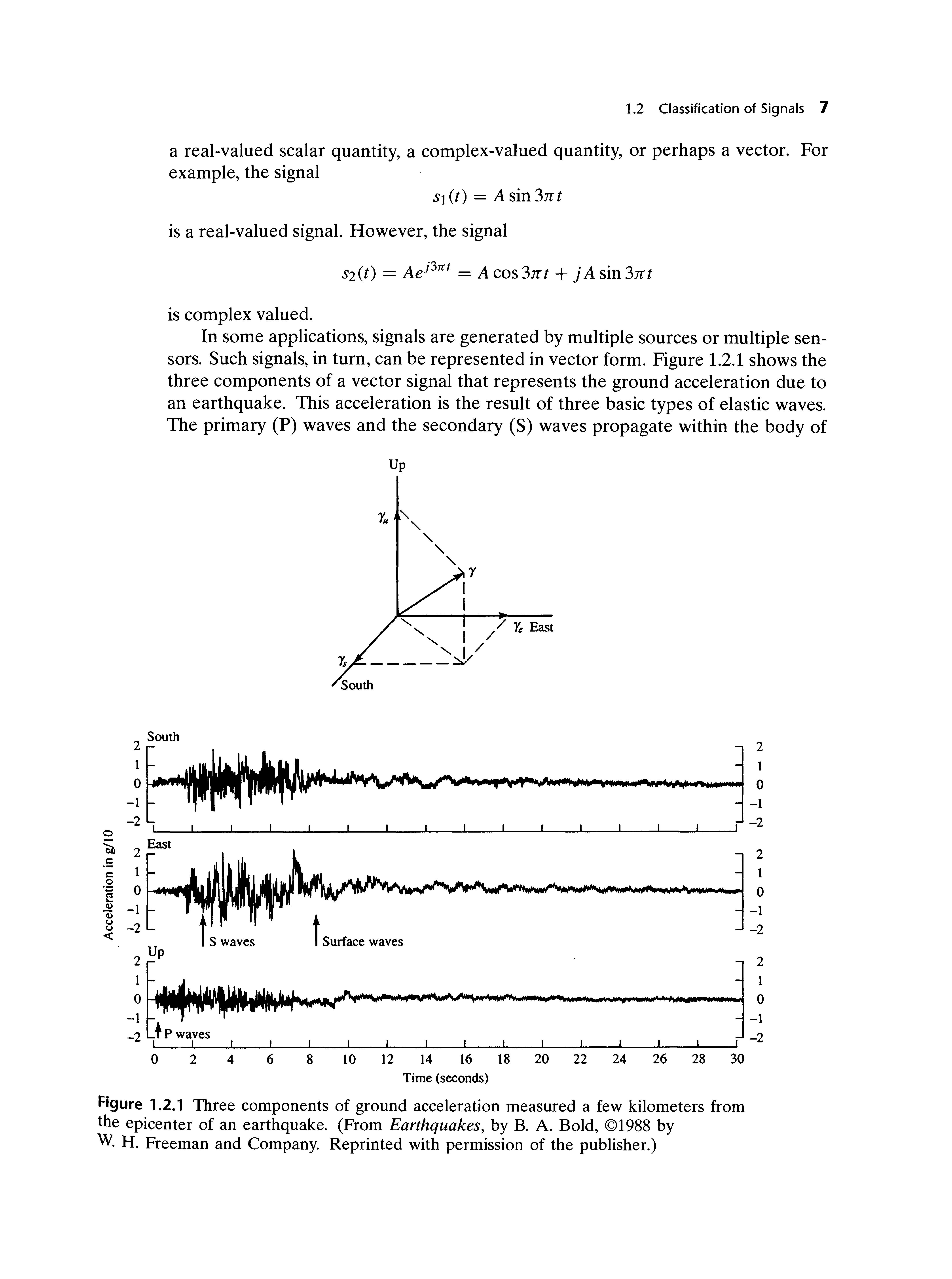
The picture shown in Fig. 1.2.2 is an example of a two-dimensional signal. since the intensity or brightness I (x, y) at each point is a function of two independent variables. On the other hand, a black-and-white television picture may be represented as I(x, y. t) since the brightness is a function of time. Hence the TV picture may be treated as a three-dimensional signal. In contrast, a color TV picture may be described by three intensity functions of the form I,. (x. y, t), IK (x, y. t), and I" (x , y. t). corresponding to the brightness of the three principal colors (red. green. blue) as functions of time. Hence the color TV picture is a three-channel. three-dimensional signal, which can be represented by the vector
[ I,. (x. V. 1) ]
I(X,y.t)= Ig(x,y.t) I" (x y. t)
1.2 Classification of Signals 9
In this book we deal mainly with single-channel, one-dimensional real- or complex-valued signals and we refer to them simply as signals. In mathematical terms these signals are described by a function of a single independent variable. Although the independent variable need not be time, it is common practice to use t as the independent variable. In many cases the signal processing operations and algorithms developed in this text for one-dimensional. single-channel signals can be extended to multichannel and multidimensional signals.
1.2.2 Continuous-Time Versus Discrete-Time Signals
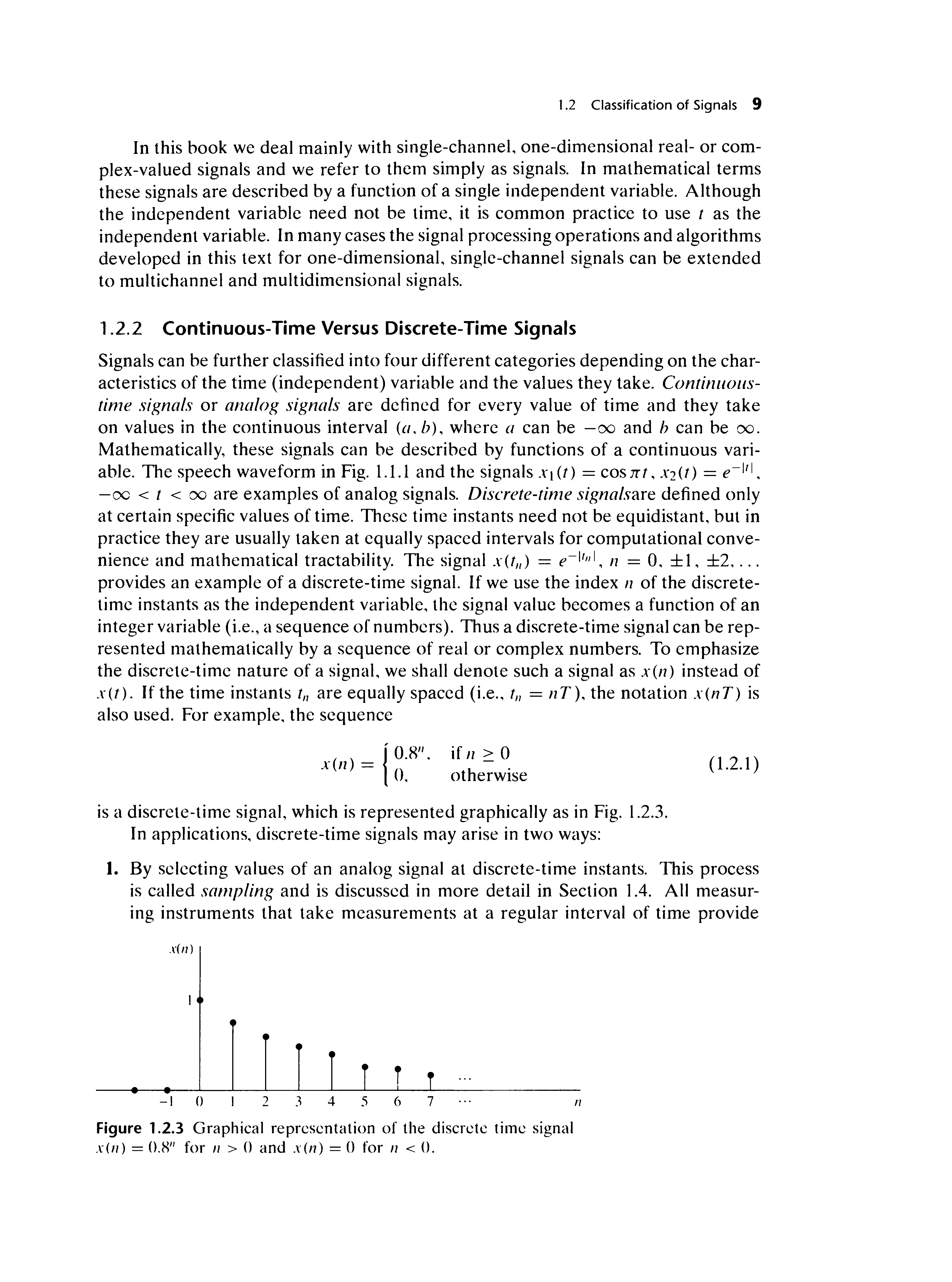
Signals can be further classified into four different categories depending on the characteristics of the time (independent) variable and the values they take. Continllollstime signals or analog signals are defined for every value of time and they take on values in the continuous interval (a, b), where a can be -00 and h ean be 00. Mathematically, these signals can be described by functions of a continuous variable. The speech waveform in Fig. 1. I.l and the signals Xl (t) = cos m , X2 (t) = e- I/I , -00 < t < 00 are examples of analog signals. Discrete-time signa/sare defined only at certain specific values of time. These time instants need not be equidistant, but in practice they are usually taken at equally spaced intervals for computational convenience and mathematical tractability. The signal X(tll) = e-I/"I, 11 = D, ±I, ±2, ... provides an example of a discrete-time signal. If we use the index II of the discretetime instants as the independent variable, the signal value becomes a function of an integer variable (i.e., a sequence of numbers). Thus a discrete-time signal can be represented mathematically by a sequence of real or complex numbers. To emphasize the discrete-time nature of a signal, we shall denote such a signal as x(l1) instead of xU). If the time instants tIl are equally spaced (i.e., til = nT), the notation X(I1 T) is also used. For example, the sequence
{ ' D.R", x(ll) = 0, if II D otherwise
is a discrete-time signal, which is represented graphically as in Fig. 1.2.3. In applications, discrete-time signals may arise in two ways: (1.2.1 )
1. By selecting values of an analog signal at discrete-time instants. This process is called sampling and is discussed in more detail in Section 1.4. All measuring instruments that take measurements at a regular interval of time provide
.1'(1/)
-I 0 2
Figure 1.2.3 Graphical representation of the discrete time signal X(II) = O.X" for II > 0 and .t(n) = () for II < O.
discrete-time signals. For example, the signal x(n) in Fig. 1.2.3 can be obtained by sampling the analog signal x(t) = O.W , t ::: 0 and x(t) = 0, t < 0 once every second.
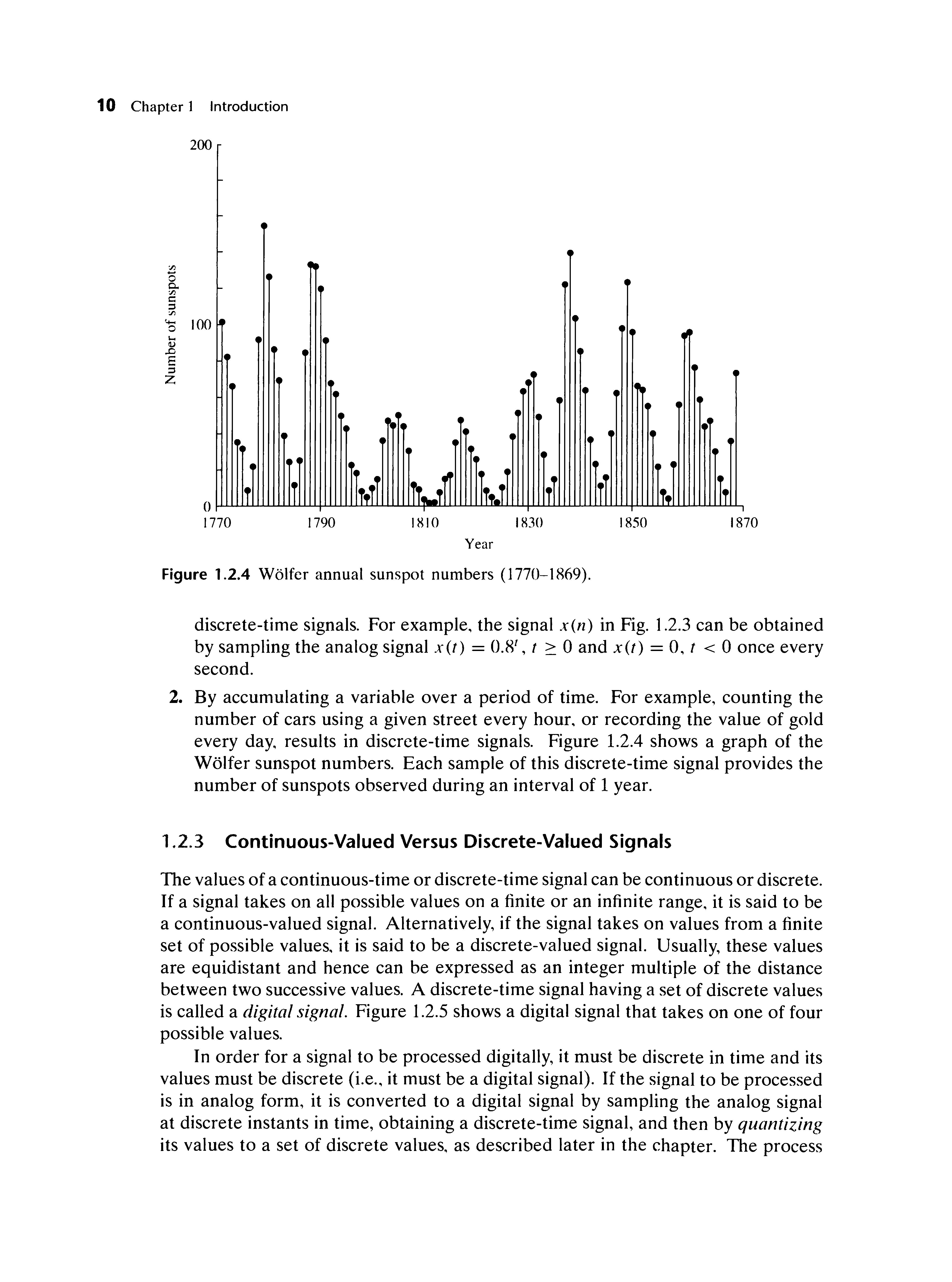
2. By accumulating a variable over a period of time. For example, counting the number of cars using a given street every hour, or recording the value of gold every day, results in discrete-time signals. Figure 1.2.4 shows a graph of the WOlfer sunspot numbers. Each sample of this discrete-time signal provides the number of sunspots observed during an interval of 1 year.
1.2.3 Continuous-Valued Versus Discrete-Valued Signals
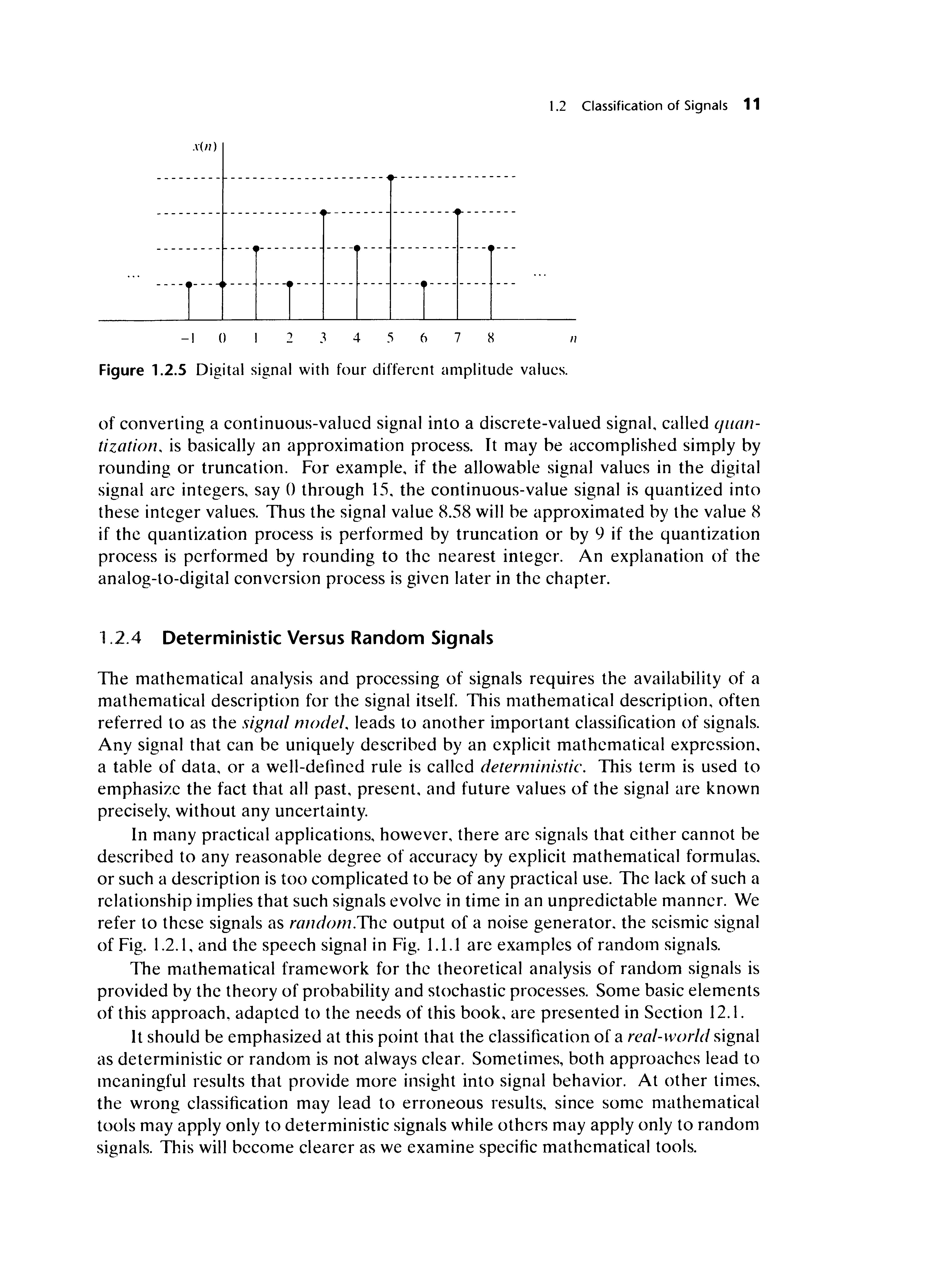
The values of a continuous-time or discrete-time signal can be continuous or discrete. If a signal takes on all possible values on a finite or an infinite range. it is said to be a continuous-valued signal. Alternatively, if the signal takes on values from a finite set of possible values. it is said to be a discrete-valued signal. Usually, these values are equidistant and hence can be expressed as an integer mUltiple of the distance between two successive values. A discrete-time signal having a set of discrete values is called a digital signal. Figure 1.2.5 shows a digital signal that takes on one of four possible values.
In order for a signal to be processed digitally, it must be discrete in time and its values must be discrete (i.e., it must be a digital signal). If the signal to be processed is in analog form, it is converted to a digital signal by sampling the analog signal at discrete instants in time, obtaining a discrete-time signal, and then by quantizing its values to a set of discrete values, as described later in the chapter. The process
1.2 Classification of Signals 11
() 2 J 456 7 H 11
Figure 1.2.5 Digital signal with four different amplitude values.
of converting a continuous-valued signal into a discrete-valued signal, called qllantization, is basically an approximation process. It may be accomplished simply by rounding or truncation. For example, if the allowable signal values in the digital signal are integers, say 0 through 15, the continuous-value signal is quantized into these integer values. Thus the signal value 8.58 will be approximated by the value 8 if the quantization process is performed by truncation or by 9 if the quantization process is performed by rounding to the nearest integer. An explanation of the analog-to-digital conversion process is given later in the chapter.
1.2.4 Deterministic Versus Random Signals
The mathematical analysis and processing of signals requires the availability of a mathematical description for the signal itself. This mathematical description, often referred to as the signal model, leads to another important classification of signals. Any signal that can be uniquely described by an explicit mathematical expression, a table of data, or a well-defined rule is called deterministic. This term is used to emphasizc the fact that all past, present, and future values of the signal are known precisely, without any uncertainty.
In many practical applications, however, there are signals that either cannot be described to any reasonable degree of accuracy by explicit mathematical formulas. or such a description is too complicated to be of any practical use. The lack of such a relationship implies that such signals evolve in time in an unpredictable manner. We refer to these signals as random.The output of a noise generator. the seismic signal of Fig. 1.2.1, and the speech signal in Fig. 1.1.1 are examples of random signals.
The mathematical framework for thc theoretical analysis of random signals is provided by the theory of probability and stochastic processes. Some basic elements of this approach, adapted to the needs of this book, are presented in Section 12.1. It should be emphasized at this point that the classification of a real-world signal as deterministic or random is not always clear. Sometimes, both approachcs lead to meaningful results that provide more insight into signal behavior. At other times, the wrong classification may lead to erroneous results, since some mathematical tools may apply only to deterministic signals while others may apply only to random signals. This will become clearer as we examine specific mathematical tools.