Using Multivariate Statistics
Barbara G. Tabachnick
California State University, Northridge
Linda S. Fidell
California State University, Northridge
Portf olio Manager: Tani maa Mehra
Content Pro d ucer: Kani Kapoor
Portf olio Manager Ass istant: Anna Austin
P roduct Mark eter: Jessicn Quazza
Art/D esigner: Integra Software Services Pvt. Ltd.
Fu ll-Service P r oject Manager : Integra Software Services Pvt. Ltd.
Compositor: Integra Software Services Pvt. Ltd
P rinter/Binder: LSC Communications, Inc.
Cover Printer: Phoenix Co/or/Hagerstown
Cover Design : Lumina Dntamntics, Inc.
Cover Art: Slnttterstock
Acknowledgments of thi rd p arty co ntent a ppear o n p ages within th e text, which constitutes an extens ion o f this co p yrigh t page.
Copyright © 2019, 2013, 2007 b y Pe arson Educatio n , I nc or i ts a f filiates. All Rights Reserved. Printed in th e United S tates of Ame rica This publication is protected b y copyr ig h t, an d pe rmiss ion s h o uld be obtained from th e publis her pri or to an y p rohibited reproduc ti on, storage in a retrieval system, or tra ns m ission in any form o r b y a ny m eans, electronic, m ech an ical, pho tocop ying, reco rding, o r otherw ise. For infom1ation rega rding p ermiss io ns, req uest forms a nd the a ppro p riate contacts within the Pearson Educatio n Globa l R;ghts & Permiss io ns d epar tm en t, please vis it www.pearson ed.com/ p e rmissions/.
PEARSON an d ALWAYS LEARNING are exclus ive trad em arks own ed by Pear son Education , Inc. or its a ffili ates, in th e U.S., and / or oth er countries .
Unless o th erwise ind icated herein, an y thir d -party trade marks th a t may appear in this wo rk are th e property o f th eir res pec ti ve owners an d an y refe rences to thir d -party trade marks, logos o r o ther trade d r ess are for dem o nstra ti ve o r descripti ve purp oses only. S ucll re fe rences ar e not inte nded to im p ly any sponsors h ip, e ndorsement, a u th oriza ti o n, o r pro m otio n o f Pearson's products b y the own ers o f s uch m ar ks, or an y rel a ti o ns h ip b etween th e owner a nd Pearson Educatio n, Inc. or its affiliates, a u thors, licensees or distrib utors.
Man y o f the d es igna ti o ns b y m a nufac ture rs an d seller to d istinguish th ei r p rod ucts are clain1ed as trademar ks. Where those designations a ppea r in th is book, an d th e pu b lish e r was aware o f a tra d emark cl aim , the d es ignations have been p rinted in initial caps o r all caps.
Lib r ary of Congr ess Catal oging-in-Publication D ata
Nam es: Tabachnick, Barb ar a G., a u th o r I Fidell, Linda S., author.
Ti tl e: Us in g mu l tivar ia te s tatis tics/Ba rbar a G. Taba cllnick, Ca liforni a Sta te U n iversity, North r i dge, Linda S. Fidell, Califo rni a Sta te U ni ver sity, Northri dge.
Descri p tion : Seventh edition I Boston : Pearso n, [2019) 1 Chapte r 14, b y Jod ie B. Ullm an
Id entifie rs : LCCN 2017040173 1 ISBN 9780134790541 I ISBN 0134790545
S ubjec ts : LCSH: Mu l tivar ia te an alysis. I Statistics.
C lassifica ti on : LCC Q A278 .T3 2019 I DOC 519 5/35--dc23
LC record ava il ab le a t h ttps :/ /lccn .loc.gov / 2017040173
1 18
Books a Ia Carte
ISBN -1 0: 0-13-479054-5
ISBN-13: 978 -0-13-479054-1
2.1 Research Questions and Associated Techniques 15
2 .1 .1 Degree of Relationship Among Varia bles 15
2.1.1.1 Bivariate r 16
2.1.1.2 Multiple R 16
2.1.1.3 Sequentia l R 16
2.1.1.4 Canonica l R 16
2.1.1.5 M ul tiway Freq uen cy Ana lys is 17
2.1.1.6 M ultileve l Mode ling 17
2. 1 2 S ig n ifica n ce o f C ro up Diffe rences 17
2.1.2.t One-Way ANOVA and I Tes t 17
2.1.2.2 One-Way ANCOVA 17
2.1.2.3 Facto ria l ANOVA 18
2.1.2.4 Factoria l ANCOVA 18
2.1.2.5 lfotelling's
2.1.2.6
2.1.2.7
2.1.2.8
2.1.2.9
2.1.3 Prediction of Group Membership
2.1.3.1 One-Way Discriminant Analysis
2.1.3.2 Sequential One-Way Discriminant Analysis
2.1.3.3 Multi way Frequency Analysis (Logit)
2.1.3.4 Logistic Regression
2.1.3.5 Sequential Logisbc Regression
2.1.3.6 Factorial Discriminant Analysis
2.1.3.7 Sequential Factorial Discriminant Analysis
2 .1.4 Structu re
2.1. 4.1 Principal Components
2.1 .4.2 Factor Ana lysis
2.1. 4.3 Stmc tural Equation Mode ling
2.1.5 Tim e Course of Eve nts
2.1.5.1 Survival/Failure Analys is
2.1.5.2 Tim e-Se ries A na lysis
2 2 So m e Furth e r Co m pa riso ns
2 .3 A Decision Tree
2 .4 Techn iq u e Chap ters
2 .5 Prelimina r y Check of the Data
Re view of Uni va riate and Bi variate S ta ti s ti cs
3.1 Hypothesis Tes ting
3.1.1 One-Sample z Test as Prototype
3.1.2 Power
3.1.3 Extensions ofthe Model
3.1.4 Controversy Surrounding Significance Testing
3.2 Analysis of Variance
3.2 1 One-Way Between-Subjects ANOVA
3.2 2 Factorial Between-Subjects ANOVA
3.2.3 Withi n -Subjects ANOVA
3.2 .4 M ixed Between-Within-S u bjects ANOVA
3.2 .5 Design Comp lexity
3 2 5.1 Nesting
3 2 5.2 Latin-Squa re Des igns
3 2 5.3 U nequa l 11 and Nonor thogona li ty
3 2 5.4 Fixed a nd Ra ndo m Eff<>cts
3.2 .6 Sp ecific Com pari so n s
3 2 6.1 We igh ting Coefficients for Comparisons
3 2 6.2 Orthogonality of We ighting Coefficients
3.2.6.3 Obtained F for Comparisons
3.2.6.4 Critical F for PLmned Comparisons
3.2.6.5 Critical F for Post Hoc Comparisons
3.3 Parameter Estimation
3.4 Effect Size
4.1.4.1
Varian ce-Covar iance Mntriccs 73
4.1.6 Common D a ta Transformations 75
4.1.7
4 .2.1 Screening Ungrouped Data 80
4.2.1.1 Accuracy of Input, Misi.ing Data,
Distribu tions, and Univariate Outliers 81
4.2.1.2 Lineari ty and Homoscedasticity
1 3 Transformation 84
4.2.1.5 Va riables Causing Cases to Be Ou tliers
Cen tering When Interactions
4.2.2.4 Variables Causing Cases to Be Outliers 94 and Powers of IVs Are Included
4.2.2.5 Multicollinearity
5.7
5.7.2
5.7.3
5.7.4
6.3.2.1
6.3.2.2 Absence of Outliers
6.3.2.3
6.3.2.4 Normality of Sampling Distributions 173
6.3.2.5 Homogeneity of Va riance 173
6.32.7 Homogeneity of Regression 173 of Variance and Covariance
6.3.2.8 Reliability o f Co ,•ariat cs 174
65.4.1 Wiiliin-Subjects and Mixed
7.4.2
7.5
7.5.1
7.5.3.2
7.5.3.3
7.5.5.2
9.3 Limitations to Discriminant Analysis 304
9.3 1 Theoretical issues 304
9.3 2 Practical issues 304
9.3.2.1 Unequal Sample Sizes, Missing Data, and Power 304
9.3.2..2 Multivariate Normality 305
9.3 2.3 Absence of Outliers 305
9.324 of Varianc:e--Covariance Matrices 305
9.3 2.5 Linearity 306
9.3 2 6 Absence of Multicollinearity and Stngularity 306
9.4 Fundamental Equations for Discriminant Analysis 306
9 4.1 Derivation and Test of Discriminant Functions
9.4.2 C lassification 309
9.4.3 Computer Analyses of Sma ll -Samp le Ex am pl e 311
9.5 Types of D iscrim ina nt Anal yses 3 15
9.5. 1 Di rect Discri min a nt An a lys is 3 15
9.5.2 Sequential D isc r imi n a n t An a lys is 3 15
9.5.3 S tepwise (S ta t is tical) Discri mina nt Ana lysis 3 16
9.6 Some Important Iss u es 316
9.6 1 Statistical l nference 316
9.6.1.1 Criteria for Overall Statistical Significance 317
9.6. 1.2 Stepping Methods 317
9.6.2 Number of Discriminant Functions 317
9.6.3 Interpreting Discriminant Functions 318
9 6 3 1 Discriminant Function Plots 318
9 6 .3 .2 Structure Matrix of Loadings 318
9.6.4 Evaluating Predictor Variables 320
9.6.5 Effect Size 321
9.6.6 Design Complexity: Factorial Designs 321
9.6.7 Use of Classification Procedures 322
9 6 7 1 Cross-Validation and New Cases 322
9 6 7 2 jackknifed Classification 323
9 6 7 3 Evaluating Improvement in Classification 323
9.7 Comp lete Examp le of Discriminan t Anal ysis 3 2 4
9.7.1 Evalua ti on of Assum pti o n s 3 25
9.7.1.1 Unequa l Sample S izes and Miss ing Da ta 325
9.7. 1.2 Mul tiva ria te No rma li ty
9.7.1.3 Linea rity
9.7.1.4 Outliers
9.7.1.5 l lomogeneity of Varian ceCovariance Matrices
9.7.1.6 Multicollinearity and Singular ity
9.7 2 Direct Discrin1inan t Ana lysis
9.8 Comparison of Programs
9.8.1
9.8.2
9.8.3
10.2 Kinds of Research Questions
12.3
12.2.1 Number of Canonical Variate Pairs
12.2.2 Interpretation of Canonical Variates
12.2.3 Importance of Canonical Variates
12.3.2.1 Ratio of Cases to IVs
12.3.2.2 Norma lity, Linearity, and
13.8 Comparison of Programs 525
13.8.1 IBM SPSS Package 527
13.8.2 SAS System 527
13.8.3 SYSTAT System 527
14 Structural Equation Mod e ling by Jod ie B. Ullman 528
14.1 Genera l Purpose and Description 528
14.2 Kinds of Research Questions 531
14.2.1 Adequacy of the Model 531
14.2.2 Testing Theory 532
14.2.3 Amount of Variance in the Variables Accounted for by the Factors 532
14.2.4 Reliability of the Indicators 532
14.2.5 Parameter Estimates 532
14.2.6 Intervening Variables 532
14.2.7 Croup Differences 532
14.2.8 Longitudinal Differences 533
14.2.9 Multilevel Modeling 533
14.2.10 Latent Class Ana lysis 533
14.3 Limitations to Structura l Equation Modeling 533
14.3.1 Theoretical Issues 533
14.3.2 Practical Issues 534
14.3.21 SampleSizeand Missing Data 534
14 3.2.2 Multivariate Norm.1lity
14 3.2.3 Linearity 535
14.3.2.4 Absence of Multi collinearity and Singularity
143.2.5 Residuals
14.4 Fundamen tal Equations for Slructura l Equat ions Modeling
14.4.1 Covariance Algebra
14.4.2 Model Hypotheses
14.4.3 Model Specification
14.4.4 Model Estimation 535 535 535 535 537 538 540
14.45 Model Evaluation 543
14.4.6 Computer Analysis of Small-Sample Example 545
14.5 Some Important Issues 555
14.5.1 Model Identification 555
14.5.2 Estimatio n Techniqu es 557
14.5.2.1 Estimation Methods and Sample Size 559
14.5.2.2 Estimatio n Methods and Nonnormality 559
14.5.2.3 Estimation Metllods and Dependence 559
14.5.24 Some Recommendations for Choice of Estim.1tion Metllod 560
14.5.3 Assessing the Fit of the Model 560
14.53.1 Comparative Fit Indices 560
14.5.3.2 Absolute Fit Ind ex 562
14 5 3 3 Indices of Proportion of Variance Accounted 562
t4.5.3 4 Degree of Parsimony Fit Indices 563
14.5.3.5 Residual-Based Fit Indices 563
14.5.3.6 Choosing Among Fit Indices 56-1
14.5.4 Model Modification 564
t4.5.4. L Chi-Squa re Difference Test 564
t4.5.4.2 Lilgrange Multiplier ( LM) Test 565
t4.5.4.3 Wald Test 569
14.5.4.4 Some Caveats a nd Hints on Model Modification 570
14.5.5 Reliability and Proportion of Variance 570
14.5.6 Discrete and Ordinal Data 571
1-1.5.7 Multiple Croup Models 572
1-1.5.8 Mean and Covariance Structure Models 573
14.6 Complete Examples of Structural Equation Modeling Analysis 574
14.6.1 Confirmatory Fac tor Analysis of the WISC 574
t4.6.1.1 Mode l Specifica tion for CFA 574
14.6.1.2 Eval u atio n of Assumptions forCFA 574
14 6 1.3 CFA Model Estimation and Preliminary Evaluation 576
14 6 1.4 Model Modification 583 1-1.6.2 SEM of Health Data 589
14 6 2 1 SE..\<1 Model Specification 589
14 6 2 2 E'•aluation of Assumptions forSEM 591
14.6.2.3 SEM Model Estimation and Preliminary Evaluation
t4.6.2.4 Mode l Modification
14.7 Compa rison of Programs
14.7.1 EQS
14.7.2 LlSREL
14.7.3 AMOS
14.7.4 SAS System
Multilevel Linear Modeling
15.1 General Purpose and Description
15.2 Kinds of Research Questions
15.2.1 Croup Differences in Means
15.2.2 Croup Differe nces in Slopes
15.2.3 Cross-Leve l In teracti ons
15.2.4 Me ta -Analysis
15.2.5 Re lative Strength of Predictors at Various Levels
15.2.6 Individual and Croup Structure
15.2.7 Effect Size
15.2.8 Path Analysis at Individual and Croup Levels
15.2.9 Analysis of Longitudinal Data
15.2.10 Multilevel Logistic Regression
15.2.11 Multiple Response Analysis
15.3 Limitations to Multilevel Linear Modeling 618
15.7.1.1 Samp le Sizes, Missing
15 3.1 Theoretical Issues 618 Data, and Distributions 656
15.3.2 Practical Issues 618 15.7.1.2 Outliers 659
15.3.2.1 Sample SUe, Unequal-11, and l\1issing Data 619
15.3.2.2 Independence of Errors 619
15.4 Fundamental Equations 620
15.4 .1 Intercepts-Only Model 623
15 4 1.1 The Model:
Level-l Equation 623
15 4 1.2 The Intercepts-Only Model: Level-2 Equation 623
15 4 1.3 Computer Analyses
of Intercepts-Only Model 624
15.4.2 Model with a First-Level Predictor 627
15 4 2 1 Level-l Equation fora Model with a Level-l 1'1\.>dictor 627
15.4.2 2 Level-2 Equations for a
Model with a Level-l Pl\.>dictor 628
15.4.2.3 Computer Ana lys is of a Model with a Level-l
15.4.3 Mode l with Predictors a t First
15.7.1.4 Independence of Errors: lntracLlss Correlations 659
Multilevel Modeling 661
15.3.2.3 Absence of Multicollinearity and Singularity 620 15.7.1.3 Multicollinearity and Singularity 659
MlwiN
and and Second Levels 633
15.4.3.1 Level-l Equation for Model with Predictors at Both Levels 633
15 4 .3.2 Level-2 Equations for Model with Predictors 16.3 Limitations to Multiway Frequency
1 Independence
at Both Levels 633 16.3.2 2 Ratio of Cases to Variables 675
15 4 .3.3 Computer Analyses of Model with Predictors at 16.3.2.3 Adequacy of Expected Frequencies 675 First and Second Le,·els 634 16.3.2.4 Absence of Outliers in the
15.5 Types of ML\11 638 Solution 676
15.5.1 Repeated Measures 638
15.5.2 Higher-Order ML\11 642
15.5.3 Latent Variables 642
16.4 Fundamental Equations for Multiway Frequency Analysis 676
16.4 1 Screening for Effects 678
15.5.4 Nonnormal Outcome Variables 643 16.4.1.1 Total Effect 678
15.5.5 Multiple Response Models 644
15 6 Some Important Issues 644
15.6.1 l ntraclass Cor relation 644
15.6.2 Cente ring Predic tors and Changes in Their In te r pretations 646
16 4.1.2 First-Order Effects 679
16.4.1.3 Second-Order Effects 679
16.4.1.4 Third-Order Effect 683
15.6.3 Interactions 648 16.4.2 Modeli ng 683 16.4.3 Eva luation and Interpretatio n 685 16.4.3 1 Residua ls 685
15.6.4 Rando m a nd Fixed In tercep ts and Slopes 648
15.6.5 Statistical Infere nce 651
15.6.5.1 Assessing Models 651
15.6.5.2 Tests of Individual Effects 652
15 6.6 Effect Size 653
15.6.7 Estimation Techniques and Convergence Problems 653
15.6.8 Exploratory Model Building 654
15.7 Complete Example of MLM 655
16.4.3.2 J>aramctcr Estimates 686
16.4.4 Compu te r Ana lyses of S ma ll -Sa mp le Example 690
16.5 Some Important Issues 695
16.5.1 H ierarchical and Nonhierarchical Models 695
16.5.2 Statistica l Criteria 696
16.5.2 1 Tests of Models 696
16.5.2.2 Tests of Individual Effects 696
16.5.3 Strategies for Choosing a Model 696
16.5.3 1 IBM SPSS Hll.OGLINEAR
15.7 1 Evaluation of Assumptions 656 ( Hierarchial) 697
16.5.3.2 SPSS GENLOG
(General Log-Linear)
SPSS LOCUNEAR (General
16.6 Complete Example of Multiway
Evaluation of Assumptions:
o f Expected Frequencies
Hierarchical Log-Linear Ana lys is
16.6.2.1 Preliminary Model Screening
16.6.2.2 Stepwise Model Se lection
Interpretation of the
Analysis
Effect Size and Power
17.3 Assumptions of Time-Series Ana lysis 718
17 3.1 Theoretical Issues 718
17.3.2 Practical Issues 718 An Overview of the General
17.3.2.1 Norma lity of Dis tributiOltS
of Residua Is 719
I7 .3.2.2 Homogeneity of Variance
and Zero Mean of Residuals 719
Bivariate to Multivariate Statistics
17.3.23 Independence of Residuals 719 and Overview of Techniques n5
17.3.24 Absence of Outliers 719 18.2.1 Bivariate Form n5
17.3.2.5 Sample Size and Missing Data 719
17.4 Fundamental Equations for
Tune-Series ARIMA Models no
17.4.1 Identification of A RIMA
(p, d, q) Models no
17.4.1.1 Trend Components, d: Making the Process Stati onary 721
Auto-Regressive Components 722
17.4.1.3 Moving Average Components 724 17.4.1.4 Mixed Models 724
17.4.1.5 ACFs and PACFs
17.4.3 Diagnosing a Model
17.4 4 Computer Analysis of Small-Sample
Types of Tune-Series Analyses
17.5.1 Models with Seasonal Components
Appendix A
y Introduction to
and
Multiplication, Transposes, and Square 1 7.5.2 Models with Interventions
A.6 Matrix "Division" (Inverses and B.7 Impact of Seat Belt Law
Determinants)
A.7 Eigenvalues and Eigenvectors: Procedures for Consolidating Variance
from a Matrix 788
The Selene Online Educational Game
C.2 Critical Val u es of th e t D istrib u tion
Research D es igns fo r Co mp le te fo r a = .05 a nd .01, Two-Tailed Test
Examples
B.1 Women's Health and Drug Study 791
C.3 Cri t ica l Va lues of the F Dis trib utio n
Crit ica l Va lues of Chi Sq uare (r)
c.s Critica l Values for Squares Multiple
B.2 Sexual Attraction Study 793 Correlation in Forward Stepwise
B.3 Learning Disabilities Data Bank
B.4 Reaction Ttme to Identify Figures 794 C.6 Critical Values for
B.S Field Studies of Noise-Induced Sleep Distribution for a = .05 and .01
Disturbance B.6 Clinical Trial for Primary Biliary
Cirrh osis
Learning Objectives
1 .1 Explain the importance of multivariate techniques in analyzing research data
1 .2 Describe the basic statistical concepts used in multivariate analysis
1 3 Explain how multivariate analysis is used to determine relationships between variables
1 .4 Summarize the factors to be considered for the selection of variables in multivariate analysis
1.5 Summarize the importance of statistical power in research study design
1 .6 Describe the types of data sets used in multivariate statistics
1.7 Outline the organization of the text
1. 1 Multivar i ate Statis ti c s: Why?
Mu lti varia te s tatistics are in creasin g ly popular techniques u sed fo r analyzing comp licated da ta sets. They p r ovide ana lysis when there are many ind ependen t va riables (IVs) and/or many dependent va riables (DVs), all correla ted w i th one another to varyin g degrees. Because of th e difficul ty in addressing compl ica ted research q u esti on s w it h u nivaria te ana l yses and beca u se of the ava ilab il i ty of h ighly developed software for performing multiva ria te ana lyses, m ultivaria te statis ti cs have become widely u sed. Indeed, a standa rd u nivaria te s tatistics course only begins to prepare a stu dent to read resea rch li terature or a research e r to p roduce it.
But how much h arder are the m u lti varia te techniqu es? Compared w i th the mul ti varia te methods, u n i varia te statis ti ca l methods a re so s tra i ghtfo r ward and nea tl y struc tured tha t i t is ha rd to be lieve they once took so much e ffort to mas te r. Ye t many resea rchers app ly and correctl y in terp re t resu l ts of in trica te anal ysis of va riance before the grand structure is apparent to them. The same can be true of multiva ria te s tatistical me thods. A lthou g h we are delighted if you ga in in s ights in to th e full multivariate general linear model , 1 we have accomp lis h ed o u r goal if you feel comfortable se lectin g and setting u p multiva ri ate a n a lyses and in te rp reting the comp u te r o u tpu t.
Mu lti varia te methods are more complex than u nivar ia te by at leas t a n order of magnitude. However, fo r the most part, th e greater comple xity requires few con ceptual leaps. Famil iar con cepts s u ch as sampling distrib utions and homogen e ity of variance s imp l y become more elab ora te.
Mu lti varia te models have not ga ined popula ri t y by acci den t-or even by s iniste r design. Th eir grow ing populari ty pa rallels the g reate r comp lexity o f contemporary research
In psych o logy, for example, we are less and less enamo red of the s imple, clean, l abora to r y s tu dy, in which pliant, first-yea r college s tu den ts each prov i de u s w i th a s ingle behavior al measure on cue.
1.1.1 The Domain of Multivariate Statistics: Numbers of IVs and DVs
Mul ti varia te statis ti ca l me thods a re an extens ion of urtivar ia te and b i varia te s ta tistics. Mul tivaria te s ta tistics are the complete or gene ral case, w h ereas univa r iate and b i varia te s tatistics are specia l cases o f the mu lti varia te model. If your des ign has many variab les, mu lti varia te techniqu es o ften let you per fo r m a sin g le ana l ysis in s tead of a seri es o f u n iva r iate or b i varia te analyses.
Variab les are r oughly dichotomized into two majo r t ypes- independen t and depen den t. Indepen dent va r iables (IVs) are the diffe ri n g condi ti ons (treatmen t vs. placebo) to whi ch you expose your research pa rticipants o r the charac te r istics (tall o r short) tha t the pa rticipants themselves bring in to the research si tu a ti on IVs are u s u ally conside red predic to r variables beca u se they predic t th e DVs-t h e response o r ou tcome va riables. Note tha t IV and DV a re defined wi thin a research context; a DV in one resear ch set ting may be an IV in another
Additi on a l te r ms fo r IVs and DVs are p red i ctor-c ri ter ion, stim ulus-response, tas kperformance, o r simply inpu t-ou tput. We u se IV and DV t hrou g h ou t this book to identify variab les tha t belong o n one s ide of an equ ati on o r the o ther, witho u t causal imp lication. That is, the te r ms are u sed for convenience ra the r than to ind ica te tha t one of the variab les caused or determin ed the size o f th e other.
The term univariate statistics refers to analyses in w hi ch there is a s ing le DV. There may be, however, mo re than one IV. For example, the amount o f social behavi o r of gradua te students (the DV) is s tud ied as a functi on of course load (one IV) and type of training in social skills to which studen ts are exposed (another IV). Anal ysis of variance is a commonly used urtiva ria te statistic.
Bivariate statistics freq u en tl y re fers to analys is of two vari ab les, where nei th er is an expe rimenta l IV a n d the desire is simp l y to stu dy th e relati onship between th e var iab les (e.g., the re la ti onship between income and amou n t of ed u cati on). Bi varia te statisti cs, o f course, can be applied in an experimen ta l settin g, b u t u s u ally they a re not. Pro to t ypical examp les of b ivari ate statistics a re the Pearson produc t- moment cor rela ti on coefficient and chi-squa re analysis. (Chap ter 3 reviews univa ri ate a n d b ivaria te s tatistics.)
With m ul tiva ria te s tatistics, you s imu ltaneou sly ana l yze m ultip le dependent and m ul tiple in dependent va r iab les. This capabili ty is important in bo th nonexperimenta l (correl a ti on al or survey) and experimental research.
1.1.2 Experimental and Nonexperimental Research
A cr itical distinction bet ween e xperimenta l and non exper imental research is whether the research er manip u la tes the levels of t he IVs. In a n experiment, the researcher has control over the levels (or condi ti ons) of a t least one IV to whi ch a participant is exposed by dete rmining wha t the levels a re, how they are imp lemented, and how and w h en cases are ass igned and exposed to them. Furth er, the experimen te r randomly ass igns cases to levels of the IV and controls all o the r in fl uential fac to rs by h ol ding them con s ta nt, cou nterbalancing, o r ran domizing their infl u e n ce. Scores on the DV are expec ted to be the same, w ithin random varia ti on, except for the in fl uence o f the IV (Shad ish, Cook, and Campbell, 2002). If there are sys tematic differences in the DV associa ted w i th levels of the IV, th ese differences are attrib uted to the IV.
For example, if groups of undergradu a tes are randomly assigned to the same ma terial bu t differen t types o f teaching techniques, and afterwar d some grou ps o f undergrad u a tes perform be tter than others, the d iffe rence in performance is sa id, w ith some degree o f confidence, to be caused by the difference in teaching technique. In this type of research, the ter ms independent and dependent have obvious meaning: the value of the DV depends on the manipula ted level o f the IV. The IV is manipula ted by the experimen ter and the score on the DV depends on the leve l of the IV.
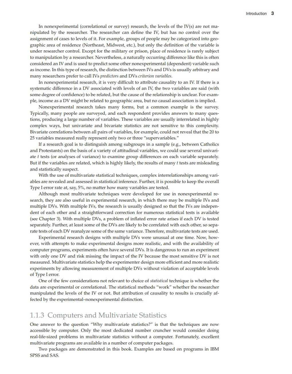
In nonexperimen tal (cor rela ti onal or sur vey) resea rch, the levels of th e IV(s) are no t manipu la ted by the research e r The resea r cher can define the IV, bu t has no con tro l over the assignmen t of cases to levels o f it. For example, groups o f people may be ca tegor ized in to geographi c a rea o f residence (Northeast, Mi dwest, etc.), b ut only the definition o f th e variable is u n der resear che r control. Excep t for the mili tary or p r ison , place of res iden ce is ra rely s u bject to manip ulation by a researche r Never theless, a naturally occurring d iffe rence like this is often cons idered an IV and is u sed to p red ict some other non exper imen tal (dependen t) variab le s u ch as in come. In t his type of research, the distinction bet ween IVs and DVs is u s u ally a r b i trary a n d many research e rs prefe r to call IVs predictors and DVs criterion variables.
In nonexperimen ta l resear ch, it is ve r y diffi cult to attrib u te ca u sa lity to an IV. lf the re is a systematic d iffe rence in a DV associated w i th levels of a n IV, the two va riables are sai d (w i th some degree o f confiden ce) to be rela ted, b ut the ca u se of the relationship is u nclea r Fo r examp le, income as a DV m i gh t be re la ted to geographic area, bu t n o ca u sa l associa ti on is implied.
Nonexperimenta l resea r ch takes many fo rms, b u t a common examp le is the s urvey. Typ ica ll y, many peop le a re s urveyed , and each responden t prov i des answers to many q u estions, producing a large number of variables. These variabl es are u s u ally in terrelated in high ly comp lex ways, bu t univaria te and b ivaria te s tatistics a re not sensitive to this comp lex ity. Biva riate correla ti on s between all pairs of va riab les, fo r examp le, cou ld n o t revea l tha t th e 20 to 25 va r iab les meas ured really represen t only two o r three "su perva ri ab les."
lf a research goal is to distinguis h among s u bgr o u ps in a samp le (e.g., between Ca th ol ics and P r otestan ts) on th e basis of a var iet y of atti tudin al va r iab les, we cou ld u se severa l u n iva riate I tes ts (o r ana lyses o f va riance) to examine grou p d iffe rences on each va r iable separately. But if the var iab les are rela ted, which is h i ghl y likel y, the resu lts of many t tests a re misleading and s tatisti ca ll y s u spec t.
Wi th the use of m ul tiva ria te s tatistical techniqu es, comp lex inte rrela ti onsh ips among va riab les a re revea led and assessed in s ta tistical inference. Fur ther, i t is poss ible to keep the overall Type I error ra te at, say, 5%, n o ma tter how many vari ab les a re tested.
Al thou g h mos t m u lti var ia te techniqu es we re developed fo r u se in nonexper imen tal research, they a re also u seful in e xpe rimen ta l research , in which there may b e m ultip le IVs a n d mul tiple DVs. With mul tiple IVs, the research is usually des igned so that the IVs are independent of each other and a str a ightfor ward correc ti on fo r n u mero u s statistica l tests is availab le (see Chap ter 3). With mul tiple DVs, a problem o f infla ted erro r ra te arises if each DV is tested separa tely. Further, a t least some of the DVs a re li kely to be correlated w ith each o th er, so separate tests of each DV reana lyze some of the same variance. Therefore, mul ti varia te tes ts are u sed. Experimen ta l resea rch des igns w i th m u ltiple DVs were un u s u al a t on e time. Now, however, w ith attempts to make experimenta l designs more rea listic, and w i th th e availab i l ity of comp ute r programs, experiments often h ave several DVs. It is dangerou s to run an expe riment w i th o n ly one DV a n d ris k missing the impact of the IV beca u se the mos t sensi tive DV is not measured. M u lti varia te s tatistics help the expe rimen ter des ign more effici en t and more realis ti c experimen ts by allowin g measu rement of m u ltip le DVs w ithout v i ola ti on of acceptab le l evels of Type I error.
One o f the few con s idera ti ons not relevan t to ch o ice of statistical techniqu e is whe ther th e da ta a re experimen tal o r cor rela ti onal. The statis ti ca l methods "wo r k" w h e the r the researcher manip u la ted the levels of th e IV or not. But attrib uti on of ca u sali ty to resu lts is crucially affected by the expe rimenta l- n onexperimen ta l d istinction.
1.1.3 Computers and Multivariate Statistics
One answer to the question "Why m u lti vari ate s ta tistics?" is that the techni ques are now accessib le by compu ter. Only the mos t dedica ted n u mber cr unch e r would cons ider doing rea l-li fe-sized prob lems in m u ltivariate statisti cs w itho u t a compu ter. Fortun ate ly, excellen t mu lti var ia te programs are available in a numbe r of compu te r packages.
Two pack ages a re demon s trated in this b ook. Examples are based o n p r ograms in IBM SPSS and SAS.
If you have access to b o th pack ages, you are ind eed fo rtun a te. P r ogra ms w ithin the packages d o not comp letely overlap, and som e p rob le ms a re b e tte r handle d through one p ackage than the other Fo r exam p le, do in g sever a l versions o f the sa m e b asic ana lysis on the sam e set of d a ta is par ticularly easy w i th IBM SPSS, w h e reas SAS has the m ost ex tensi ve capab iliti es for sav ing deri ved sco res fro m d a ta screening o r fro m in term ed i ate a n a lyses.
C hap ter s 5 thro u g h 17 (the chap te rs th a t cover th e specialized m ulti va ria te techni ques) offer expl anations an d ill ustra ti ons of a variety of p rogra m s 2 wi thi n each package and a co mpa r ison of the fea tu res o f the p r ogra ms. We hop e tha t once you un derstand the techniques, you wi ll b e a bl e to generalize to v i r tua ll y any multiva riate progra m
Recen t ve rsions o f th e progra m s a re availa b le in Win dows, with m en u s tha t im plem e n t m ost o f th e tech n i q u es ill u s tr a te d in this b ook. A ll of t he techniques m ay b e i mp le m en te d thr o u g h syn tax, and syn tax i tself is gene rated through m en u s. Then you m ay add o r ch ange syn tax as d es i red for your ana lysis. For examp l e, you may "pas te" m enu cho ices in to a syn tax win dow in IBM SPSS, e d i t the resu l ting tex t, and th en run th e progra m . Also, syn tax gen era ted by IB M SPSS m enus is saved in the "journ a l" fi le (s ta ti s t ics.jnl ), which may also b e accessed and cop ied in to a sy n tax window. Sy n ta x gen e ra te d b y SAS menu s is reco rded in a "log" file. Th e con ten ts m ay then b e copi ed to a n in te rac ti ve w in dow, e d ite d , a n d run . Do no t ove rl ook the he lp fi les in th ese p rograms. In d eed, SAS and IBM SPSS now p rovid e the en tire set of user m an u a ls o n l in e, often w i th m ore cu rren t info rmat ion th an is availa b le in printed ma n uals.
O u r IBM SPSS demons trati ons in this book a re b ased on syntax generated throu gh menus whenever feasib le. We wou l d love to show you the sequ ence of m en u choices, b ut space d oes no t permit. And , fo r the sake of pa rsimon y, we h ave ed ited p rogram o u tpu t to ill u s trate the m a te ria l that we feel is the m ost importa nt fo r in te rpre tation.
With comm e rcia l computer packages, you need to know whi ch vers ion o f the pack age you a re usin g. P rograms a re con tin u a ll y be in g changed, and n o t a ll changes a re immed iately implem en ted a t each faci li ty. Therefo re, m a n y versions o f the var iou s p rograms are s im u ltaneou sly in use a t different insti t utions; even a t one ins ti tuti on , mo re than one ve rs ion of a pack age is som e times availab le.
Progra m u p da tes are o ften correcti on s of err ors discovered in earl ier vers ion s. Som e tim es, a new vers ion w ill change the o utp u t fo rm at bu t n o t i ts info rma ti on Occasionally, thou gh, there a re m ajo r revis ions in o n e o r m o re programs or a new program is added to the p ackage. So me tim es d efau lts change w i th u p d a tes, so tha t the ou t pu t looks diffe rent although syntax is the sa m e. Check to find ou t whi ch vers i on of each package you a re u sin g. Th en, if you a re u s in g a p r in ted m anu al, be su re tha t the m anua l you a re using is consis ten t w i th the vers ion in u se a t you r facil ity. Also chec k u pdates for error cor recti on in prev i ou s releases th a t may be relevant to so m e of your p rev iou s run s.
Excep t whe re no ted, this b ook reviews Wind ows versions o f IBM SPSS Vers ion 24 and SAS Version 9.4. Info rm ation on avai lab ility and versions of software, macros, books, and the like changes a lmost dail y. We reco mme nd the In te rn e t as a sou rce of " keeping u p."
1.1.4 Garbage In, Roses Out?
The trick in m u l ti va ria te s tatisti cs is not in co mpu tation. This is easi ly d one as discu ssed above. The tri ck is to se lect re liab le and va lid m easure m ents, ch oose the appropria te p rogram, use it co rrectly, an d kn ow how to in te rp ret the ou tput. Ou tpu t fro m comme r cial co mpu te r p rogra m s, wi th the ir bea u tifull y fo rm atted tables, graphs, and m a trices, can m ake ga rb age look l i ke r oses. Thro u g h ou t t his b ook, we try to s u ggest cl ues that revea l when the tru e m essage in the o u tpu t m o re close ly resem b l es the fertilize r than the fl owe rs.
Second , when you use multivar ia te s tatis tics, you r a rely ge t as close to the raw da ta as you d o when you app ly uni va ria te statis ti cs to a re la ti vely few cases. Er ro rs and ano m alies
2 We have re ta ined d escrip tions of features of SYSTAT (Vers ion 13) in these sections, d esp ite the re moval of detailed dem ons trations of that progra m in this edition.
in the d a ta tha t wou ld b e ob v ious if th e data we re p rocessed by hand a re less easy to spot when processing is entire ly by comp u ter. Bu t the compu ter p ackages have progr ams to g r a p h and descr ibe you r da ta in the simp lest uni vari a te te rms and to disp lay b i varia te re la ti on shi ps a m on g your variab les. As discussed in Ch a p ter 4, these p rograms p rov ide p reliminary anal yses tha t ar e abso lu te ly necessa r y if the results of m u l ti varia te programs are to be bel i eved.
Th e re a re also certa in costs associ a ted w i th the benefi ts of usin g m u l ti variate p roced u res. Benefi ts o f in creased fle xi bi li ty in research des ign, for in s ta n ce, are som etim es pa ralleled b y in creased ambiguit y in in te rp retati on o f resul ts. In add iti on , mu l tivar ia te res u l ts can be q ui te sensi tive to whi ch a n a lyti c s trategy is chosen (cf. Section 1.2.4) and d o not a l ways prov ide better p rotection again s t s tatisti ca l errors than thei r u ni va riate cou nter par ts. Add to t his the fac t tha t occas iona ll y you s till cannot ge t a firm statis ti ca l a n swer to your research q u es ti ons, a nd you m ay wond er if th e increase in complex i ty and diffi cu lty is war ranted.
Frankly, we think it is. Sl ip per y as som e of the concepts and p rocedu res are, these s ta tistics p rovid e insig h ts into relati on shi ps amon g var iables that m ay more cl osely resemb le the comp lexity o f th e " real" worl d. And so m etimes you get at least par tia l answers to q u es ti ons tha t cou l d not b e as ked a t a ll in th e univa r iate fra m ewor k . Fo r a comp le te analysis, m a king sense of your da ta u sually requires a ju dici ous mix o f multiva r iate a n d u niva ria te statisti cs.
Th e a d diti on of m u lti varia te sta tis tica l m e th od s to your rep ertoi re makes da ta analysis a lot more fu n. If you l iked u n iva r iate s tatistics, you w ill l ove m u l ti va r ia te statistics!3
1.2 So me U s eful Definitions
In o rd er to des crib e m u l ti va ria te s tatistics easi ly, i t is u sefu l to review some co mm on terms in resear ch d es ign a n d b asic s ta tistics. Dis tincti ons were m ade b e t ween IVs and DVs and be tween exp erim enta l a n d nonexperimen ta l resea rch in precedin g sec ti ons. Ad d i tiona l terms tha t a re e n countered rep ea tedly in the book b u t n o t n ecessa rily rela ted to each other a re d escr ibed in this section.
1.2.1 Cont inuo u s, Discrete, and Dicho
t omous D a t a
In appl ying statis ti ca l techniqu es of any sort, it is impor ta n t to consid er the type of meas urement and the n a ture of the cor resp ondence be tween the nu m bers and the events tha t th ey rep resent. The distincti on m ad e here is a m on g con tinu ou s, discre te, and dich o tomous va ria b les; you m ay p refe r to s ubs ti tu te the te rms interval o r quantitative fo r continuous and nominal, categorical or qualitative for dichotomous and discrete.
C on tinuou s va r iab les a re m easured o n a sca le tha t ch anges valu es s m oothl y rather than in s te p s. Continu ou s va riab les ta ke on any va lu es wi thin t h e range of the sca le, and the size o f t h e n umber reflects th e am ou n t of the va riab le. Precision is limited b y the m easu ring ins trumen t, not by the nature of th e sca l e itself. Some exa mp les of con tin uous va riab les a re time as m eas ured on an o ld-fashion ed ana l og cl ock face, ann u a l in co m e, age, te mpera tu re, d is ta n ce, a nd grade poin t ave rage (GPA).
Discre te variab les take o n a fi n i te and u s u a ll y s m a ll nu m ber of va lu es, a nd th e re is n o s m ooth transi ti on fro m o n e va lu e o r category to the next. Examp les in clu de time as displayed b y a digital cl ock , con tinen ts, ca tego ries o f rel igiou s a ffilia ti on , and t ype of communi ty (ru ra l o r urban).
So m e tim es discrete va riab les a re u sed in mu l tiva ria te analyses as if con tinu ou s if th er e a re n ume r ous ca tego ries and the ca tegor ies represen t a q uan ti tative a t t r i bu te. Fo r ins tance, a va r ia b le tha t represents age ca tego ries (wh e re, say, 1 s tan ds fo r 0 to 4 years, 2 s tand s fo r 5 to 9 yea rs, 3 stands fo r 10 to 14 years, a n d so on u p throu gh t h e n o r m a l age s p an) can b e u sed beca u se there are a lot of ca tego ri es and the n umbe rs designa te a q u anti ta tive a ttrib u te (increasing age).
Bu t the sa m e num be rs used to designa te ca tego ries of religious affil ia ti on are not in a p p ropria te
3 Do n't e\'en think about it.
fo rm fo r analys is w ith many o f the techniqu es 4 because rel igions do n o t fall a l on g a q u an ti tative con tin u um
Discrete va riables comp osed of q u al ita ti ve ly differen t categories are so m e tim es ana lyzed after b e ing changed into a n umbe r of d ichotom o u s or t wo- level va riables (e.g., Ca th olic vs. non -Ca t h o l ic, Pro testant vs. non-P r otestan t, Jewish vs. non -Jew is h , and so on un ti l t h e degrees of freedom are u sed). Reca tego riza ti on of a d iscrete variab le in to a seri es of d icho tomous ones is ca lle d dummy variable coding T he conversion of a discre te varia b le in to a ser ies o f dich o tomous o n es is done to limi t th e rela ti on s h i p b e t ween the d icho to m ous vari ab les and o th ers to linear relationships. A discre te var iable w i th more than t wo ca tegor ies can have a rela ti onship of any s h ap e w ith anothe r var iable, and the rela ti onship is ch anged a rb itr ar il y if t h e assignm en t of nu m bers to categor ies is changed. D ich o tomo us varia b les, h owever, w i th o nl y two points, can have only linea r rel a ti on s h ips wi th o the r var iables; they are, th e refore, a p p rop ria tely a n a lyzed b y m ethods u sing co rre la tion in w hi ch o nl y linea r relationships are a n a lyzed
Th e disti ncti on between con tin u o u s and discre te variab les is not always clear. If you ad d en o u g h digi ts to the digital clock, fo r instance, i t becomes for all p rac ti ca l p u r p oses a contin uous m easu r ing dev ice, whereas time as m easu red b y the analog dev ice can a lso be rea d in discrete ca tegor ies s u ch as hou rs or half ho urs. In fact, any contin u ou s meas ure m en t m ay b e rend ered discre te (or dich otomous) w ith som e loss o f infor m a ti on, b y specifying cu toffs on the con tinu ous scal e.
Th e p roper ty of var iab les tha t is crucial to the appl icati on of m u lti var ia te p rocedures is no t the typ e o f m eas ure m en t so much as th e shape of dis tr ibu ti on, as d iscu ssed in Ch apter 4 and in discu ssi on s of tes ts o f assu mp tions in Chap ter s 5 thr o u g h 17. Non-n o rma ll y d is trib u ted con tinu ous va riab les a n d dich o tomo us va riables with very u neven sp li ts between the ca tegor ie s p resent prob lems to sever al o f th e mul ti vari a te ana lyses. This issu e and i ts resol u ti on a re discussed at some length in Cha p ter 4.
Another typ e of m eas urem en t that is u sed som etimes produces a rank o rde r sca le. This sca le assigns a nu m ber to each case to ind icate the case's posi tion vis -a -v is o th er cases along som e d im ensi on For ins tance, ranks are ass igned to con testa n ts (fi rs t p lace, second p lace, third place, e tc.) to p r ovid e a n ind ication of w h o is the bes t-b u t not b y h ow mu ch. A p roblem wi th rank order m easures is tha t the ir d is trib u tions a re rec ta n g ula r (one freq u e n cy per n umb e r ) instead o f n o rma l, u nless tied ranks a re permi t ted and they p il e up in the mi d dle of the distributi on
In p r ac tice, we often trea t varia b les as if th ey a re con tinu ous w h en the u n derl y ing scale is though t to be con tinu ous, bu t the m eas ured sca l e actu a ll y is r a nk o rd e r, the n um be r of ca tego ri es is large-s ay, seven o r m ore, a n d the da ta m eet o th e r assumption s o f the ana l ysis. For in s tance, th e n um be r o f correc t i te m s o n a n obj ec ti ve test is techni ca ll y not con tinu ou s beca u se fr actiona l va lu es a re n o t possib le, b u t i t is t h ou gh t to measure so m e u nd e rl yin g con tinu ous varia b le such as cou rse m as te r y. Another e xa m p le of a va riab le w i th a mbi guou s measurem en t is one m eas ure d on a Like rt - t ype sca le, in which cons ume rs ra te th e ir a ttitud es towa rd a p roduc t as "s tro n g ly l ike," " m ode ra te ly like," " mil d l y li ke," "nei the r like nor dis li ke," " mil d ly disl i ke," " m oderately disl i ke," o r "st r ong ly d isl ike." As m en tioned previou s ly, even d ichotom ou s va riab les may b e tr eated as if con tin u ou s und er som e con d i ti ons. Th us, we o fte n u se the te rm continuous, t h rou ghou t the rem aind er of t h is boo k, w h e ther the m eas ured sca le itself is con ti n u ou s o r the va riab le is to b e treated as if con ti n u o u s. We u se the te rm discrete fo r va r ia b les w i th a few ca tegor ies, whether th e categor ies differ in t ype o r q u antity.
1.2.2 Samples and Populations
Sam p les a re measure d to make generalizati ons abou t p o pu la ti on s. Idea lly, samp les a re se lected , usua lly b y some ran dom p rocess, so tha t they rep resen t the popu lati on of in terest. In rea l life, however, popula tions a re frequen tl y bes t defined in terms o f sam p les, ra t h e r th an vice ve rsa; the p opu la ti on is the grou p from w hi ch you were ab le to rand o mly sa mp le.
4 Som e multi varia te techniques ( e.g., logistic regression, SEM) are appropria te for all types o f va riables
Samp ling has somewhat differen t connotations in nonexperim en ta l and experim en ta l resear ch In n onexpe rimenta l research, you investi gate re la ti on s hi ps am on g varia b les in so me p redefined popu lation. Typ ica lly, you take el ab o r a te p recau ti ons to ensure tha t you h ave achieved a representa ti ve samp le of tha t popula ti on; you d efin e your popul ation, a nd then do your best to random l y sa mp le from i t.5
In expe rim enta l resea rch , you atte mp t to create differen t popu la ti ons b y trea ting subgrou ps fr o m a n originally ho m ogeneou s grou p diffe rentl y. The samp ling o bjecti ve here is to e n s ure tha t a ll cases co m e fro m the sa me popu lation b e fo re you tr ea t them differen tl y. Rand o m samp ling consists of randoml y assigning cases to treatmen t g rou p s (levels o f the IV) to ensu re tha t, b e fo re differen tial t reatmen t, a ll s ubsa m ples co m e fro m the sa m e popula ti on. Statisti cal tests p rovid e evid ence as to whether, afte r trea tm ent, a ll samp les still come from the same pop ulation. Generalizations a b o u t trea t m en t effec ti veness a re m ade to th e t ype of indiv idua ls w h o par ticipa ted in th e exper imen t.
1.2.3 Descriptive and Inferential Statistics
Descr iptive s ta tistics d escr ibe sa mp les o f cases in terms of va riables or combin a tions of variab les. Inferential statis ti ca l techniques tes t hypotheses abou t diffe rences in popul ations on the basis o f measure m ents m a d e on sa m ples of cases. If s ta tistically significan t d iffe rences are fou nd , descrip ti ve s tatisti cs a re then used to p r ovid e estima tions of cen tral tenden cy, a nd t h e l ike, in the pop ul ation. Descripti ve s ta tis tics u sed in t his way a re ca lled parameter estimates. Use of inferen ti al and d escr iptive s tatis tics is r a rely an e i ther-o r p rop osi ti on We a re usu a ll y in teres ted in both describ ing and ma king inferences abou t a d a ta set. We d escr ibe th e da ta, fi n d s ta tistica lly s ignifi can t d iffe rences o r rela ti onship s, and estim ate p opu la ti on valu es for those findings. H oweve r, the re are m o re res tr icti on s on inferen ce tha n there a re o n d escr i pti on. Many assump ti ons of multi va r iate statisti cal m e th od s a re necessary o nly for inferen ce. If simple d escr i p tion of the sam p le is t h e m ajo r goa l, ma n y ass ump tions a re relaxed , as discu ssed in Chap te rs 5 through 17.
1.2.4 Orthogonality: Standard and Sequential Analyses
O rthogona l it y is a p er fect nonassociation b e t ween varia b les. If two variab l es a re ort h ogon al, knowing the va l ue o f o n e va r iab le gives no clue as to th e valu e of th e o the r; t h e co rre l ation b e t ween the m is ze ro.
O rthogona l it y is often desi rab le in s tatisti cal applica ti ons. Fo r instance, fac to rial designs fo r e xp erim ents are orthogon al when two o r more IVs are completel y crossed w ith equ a l samp le sizes in each co mbina ti on of leve ls. Excep t for use of a common erro r term, tests of hypotheses a b o u t main effec ts and in te rac tions a re ind ependen t o f each o th e r; th e ou tcome o f each test gives n o hin t as to the ou tcome o f the o the rs. In o rt hogona l exp e rimen ta l d es igns wi th random assignm en t of cases, m anipul a ti on of the levels o f the IV, and good controls, changes in va l ue of the DV can be una m b ig u ously a ttrib u ted to var iou s ma in effec ts and in te rac tions.
Simila rl y, in mul ti varia te ana lyses, the re are a d vantages if sets o f IVs or DVs are o rthogonal. If a ll pairs of IVs in a set are o rthogonal, each IV a d ds, in a simp le fashion, to p red ic ti on of th e DV. C ons ider in com e as a DV w ith e d uca tio n and occu p ational p res ti ge as IVs. If ed u ca tion a nd occu pa tional p restige a re orthogonal, and if 35% of t h e va riabili t y in in come m ay be p red icted fro m ed u ca ti on a nd a d iffere n t 45% is pred icted fro m occu pa ti on a l prestige, then 80% of the var iance in income (the DV, Y) is predicted fr o m edu cation and occu p a tional p res ti ge together.
O rthogona l it y can eas il y be ill ustra ted in Venn diagra m s, as s h ow n in Figure 1.1. Venn d iagrams represent shared va riance (or correl a ti on ) as overlappin g a reas b e t ween two (or m o re) ci rcl es. Th e total vari ance fo r in come is one circle. The secti on w i th horizon ta l s trip es re p resents the pa rt o f income p red ictab le fr o m educa ti on (t h e firs t IV, X1), a nd t h e sec ti on w i th
5 Strategies fo r random sam pling are discu ssed in m any sources, inclu d ing Levy and Lem ens how (2009), Rea and Par ke r (1997), an d de Vaus (2002).
Fi g ure 1 . 1 Ven n di a gra m for Y (income), X, (ed u c atio n), a nd X2 (o cc upatio nal p rest ig e)
vertica l s tri p es represents the par t p red ictable from occu pa ti on al pres tige ( th e second IV, X2); the ci rcle fo r ed u cation overlaps the circle fo r in come 35% and the circle for occupation a l prestige overlaps 45% Toge the r, they accoun t for 80 % of th e variab ili t y in income beca u se education and occup a ti on a l p restige a re o rthogonal and do n o t themsel ves overl ap. The re are s imi lar a d van tages if a set o f DVs is o rthogona l. The overa ll effec t of an IV can be pa rtitioned in to effec ts on each DV in an add iti ve fashi on.
Usu ally, however, the variab les are cor related wi th each other (n on orthogon al). IVs in nonexper imental d es igns are often cor related na tur ally; in experimental designs, IVs become co rrel a ted wh en unequal numb ers of cases are measured in different cells of the design. DVs are u sually correla ted becau se indi vidual differences among particip ants tend to be con sis ten t over many attribu tes. When va riab les are corre l a te d , they have s h a red o r overlapping va r iance. In the e xample of Figu re 1.2, ed u cation and occupationa l p restige co rrel ate w i th each o the r. Alth ou g h th e in dependen t con tr ibuti on made by educa ti on is s till35% and th at by occupationa l prestige is 45%, their join t contrib u tion to p redic ti on of income is no t 80%, bu t ra the r somet hing s m alle r d u e to the overlapping a rea s h ow n by th e a rrow in Figure 1.2(a). A major dec is i on fo r the mu lti var ia te analyst is how to handle th e va ri ance tha t is predic ta bl e fr om m o re tha n o n e va riable. Many m u l tiva r ia te techrUqu es have at least two s trategies fo r handli n g it, bu t some have m o re. In s tanda rd analysis, the ove rlapping variance cont rib u tes to the size of s u mmary s ta tistics of the overa ll rela ti onship bu t is not ass igned to e ither variab le. Overlapping variance is disregarded in assessing the con trib u tion of each va r ia bl e to the sol u ti on. Figu re 1.2(a) is a Venn d iagra m of a standard ana lysis in w h ich overlapping var ian ce is shown as overlapping areas in circles; the u ni q u e con tr ibu ti ons o f X 1 and X 2 to p red icti on o f Ya r e s h ow n as hor izon tal and ver tica l a reas, respectivel y, and the to tal rel ationship between Y and the combin ation of X1 and X2 is those two a reas plus the a rea w ith the a r r ow. If X1 is ed u cation and X2 is occu pa ti on a l p res ti ge, th en in s tanda rd analy s is, X1 is "cred ited w ith" the area m arked b y the horizon ta l lines a n d X2 b y the a rea mark ed by ve rtica l l in es. Neithe r o f the IVs is assign ed the area d es ignated w ith the arr ow. When X 1 and X2 s ubs tantia lly overlap each o ther, very li tt le h o rizonta l or verti ca l a rea may be left fo r ei the r o f th em, desp ite the fact tha t th ey are both re la ted to Y. Th ey have essen tially knock ed each other o u t of the sol u ti on.
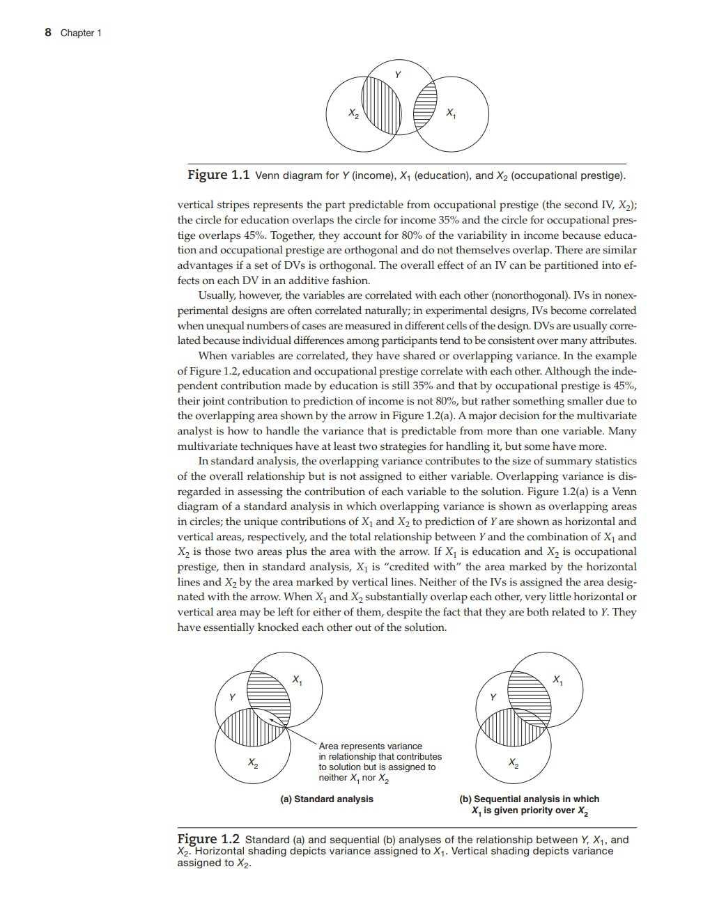
Ar ea represe nts va rian ce in relatio nship th at contr ibute s to solutio n but is assigned to neither x, nor x2
(a) Stand ard analysis
(b) Sequential analy s i s in which X 1 is g ive n p r iority ove r X2
Fi gure 1. 2 S tand a rd (a) a nd s eq uent ia l (b) a n a lys e s of t he re lat io nsh ip between Y. x, , and X2 Horizonta l s had in g d e picts varia nce as sig ned to X1 Vert ic a l s h a d ing dep icts va ri ance ass ig ned to X2
Sequ ential ana lyses differ, in tha t the researcher ass igns priority for en try of variab les in to equ a tions, and the firs t one to ente r is assigned both uniqu e variance a nd any overlapping variance it has w ith othe r variab les. Lower-pri ori ty variables a re th en assigned on en try their uniqu e and any remaining overlapping variance. Figure 1.2(b) sh ows a sequential analysis for the same case as Figure 1.2(a), w h ere X1 (ed u ca tion) is g i ven priority over X2 (occupation al p res tige). The to tal variance explained is the same as in Figure 1.2(a), b u t the rela ti ve contri b u tions of X1 and X2 h ave changed; education now shows a s tronger relationship wi th in come than in the standard anal ysis, whereas the rela tion b etween occupa ti ona l pres tige and income remains the same.
The choice o f stra tegy for dealing with ove rlapping variance is not trivial. If va ri abl es are correla ted, the overa ll rela ti on ship remain s the same, but the apparent importance of variab les to the sol u ti on changes dependin g on whe the r a s ta n dard or a sequ entia l s tra tegy is u sed. If the mul tiva ri a te p r ocedu res have a repu ta ti on for unreliability, it is b ecause sol u ti on s change, sometimes d r amati cally, w h en differen t s tra tegi es fo r entr y of var iables a re chosen. Howeve r, the s tra tegies also ask different q u estions of the da ta, and it is in cumbent on the research e r to de termine exactl y w hi ch ques ti on to as k . We try to make the ch o ices clear in the ch apte rs tha t follow.
1.3 Linear Combinations of Variable s
Mu lti varia te a n a lyses combine variables to do usefu l work, s u ch as p red ict scores o r p red i ct grou p memb e rship. The comb inati on that is fo r med depends on th e rela ti onships among the variab les and th e goals of analys is, bu t in most cases, th e combina ti on is lin ear. A linear combina ti on is one in w hi ch each variab le is ass ig n ed a we ight (e.g., W1), and then the p roduc ts of weights and the va r iab le sco res are s u mmed to pred ict a score on a combin ed va ri ab le. In Equ ati on 1.1, Y' ( the pred icted DV) is predic ted by a l in ea r combin a ti on of X1 and X2 ( the IVs).
(1.1)
If, for examp le, Y' is p red icted income, X1 is educa ti on, and X2 is occupationa l prestige, the best p red iction of income is obtain ed by weighting educa ti on (X 1) by W1 and occupa ti on al prestige (Xv by W2 before s u mming. No o the r va l ues of W1 and W2 prod u ce as good a p red icti on o f income.
Notice tha t Equa ti on 1. 1 includes nei the r X 1 nor X2 r aised to powe rs (expon en ts) n o r a prod u ct o f X 1 and X2 Th is seems to severely restric t mul ti va ria te sol u ti ons u n til o n e realizes tha t X1 cou ld i tself be a p r od u ct o f t wo diffe rent variab les or a single variab le r a ised to a power For examp le, X1 migh t be educa ti on squ a red. A mu lti var ia te sol uti on does no t prod u ce exponents o r cross-prod u cts of IVs to improve a so lu tion, but the resea r ch er can inclu de Xs tha t are cross-prod u cts of IVs or a re IVs ra ised to powers. Inclusion o f variables raised to powers o r cross-produc ts of vari ab les has bo th theoretica l and p rac ti ca l impl icati ons fo r the so lu tion. Ber ry (1993) p rov ides a useful discu ssion o f many of the issues.
Th e s ize o f the W va lu es (o r some function of them) o ften reveals a great deal abou t th e relati on ship between DVs and IVs. If, fo r ins tance, the W valu e fo r some IV is zer o, th e IV is not needed in th e bes t DV- IV re l ationship. Or if some IV has a large W va lue, th en the IV tends to be important to th e relationship. A lthou g h comp l ica ti on s (to be expl ained l a ter) prevent inte rpreta ti on of the multiva riate solu tion from the sizes o f the W valu es alone, they are nonetheless impo rtan t in most multiva r iate p r ocedures.
Th e combin ation o f variables can be consi dered a s u pervari ab le, n o t d irectly meas u red but worth y o f interpreta ti on. Th e s u pervariab le may rep resen t an unde rl y ing d imen s ion tha t pred i cts something or optimizes some rela ti onsh ip. Therefore, the attemp t to unders tand th e meaning of the comb ination o f IVs is worthwhi le in many m u l ti vari ate ana lyses.
In the search for th e b est weig hts to apply in comb ining variab les, compu ters do not try o ut all possib le se ts of weights. Va ri ou s a lgo ri t hms have been deve loped to compute the weigh ts. Most a l go ri thms in vol ve manipul ation of a correla ti on matrix, a va riance-covariance ma tr ix, o r a s um-of-squ a res and cross-produc ts ma trix. Section 1.6 descr ibes these ma trices in ver y
simp le te r ms an d s h ows th ei r deve lopmen t fr o m a ve r y s m all da ta set. Append ix A descr ibes some te rms and m anip u la ti ons appropria te to matrices. In the fo u r t h sections o f Cha p ters 5 through 17, a sma ll h yp o thetical sa mp le o f d a ta is analyzed b y h and to show h ow the wei ghts a re d er ived for each analysis. Thou g h this infor ma ti on is u seful for a basic unders tanding of m u l tiva ria te s ta tistics, it is not n ecessa r y fo r applying m u l ti va ria te techniqu es fru itfull y to your resea rch q u esti ons a n d may, sad ly, b e skipped by those w h o a re ma th aver se.
1.4 Number and Nature of Variable s to Include
Atten ti on to the numb er o f variab les incl uded in a n analys is is important. A genera l rule is to get the best so luti on with the fewes t variab les. As more and more var iab les are includ ed , the solu tion usually imp roves, bu t only sl ig htl y. So me times the imp rovement d oes no t compensa te for the cos t in degrees of freed om of including m ore variables, so the power of the a n alyses diminishes. A second p rob le m is averjitting. With overfitting, the solu tion is ver y good; so good , in fac t, tha t it is unlikel y to generalize to a population. Overfitting occurs when too many variab les are includ ed in an analysis rel a ti ve to the sam p le size. Wi th smalle r samples, ver y few variables can b e analyzed. Gen erally, a researcher sh o ul d incl ude o nl y a limited numb er o f uncorrela ted variables in each analysis,6 fewer w i th s mall er samples. We g i ve gui delines fo r the numb er of variab les that can b e incl uded rela tive to sam p le size in the third sections of Ch apters 5 through 17. Add iti on a l con s idera ti ons fo r incl usi on o f varia b les in a multiva riate ana lysis includ e cos t, ava i labil it y, mean i n g, and theoretica l re lati on shi ps amon g th e va ria b les. Except in a n alysis of s tru ct ure, one us u a ll y wan ts a sma ll n um be r o f valid , cheap ly ob ta ined , eas ily ava ilab le, uncorrela ted var iab les tha t assess a ll the th eore tica lly im portan t d im ensi on s of a resear ch area. Another impo rtan t con s ider a ti on is reliab il i ty. H ow s table is the p osi ti on of a g i ven sco re in a distributi on o f sco res when meas ured a t diffe rent times o r in differen t ways? Unre liab le va r iab les d egra d e an analysis, whereas relia b le o n es enhance it. A few reli ab le var iab les give a m o re m eaning ful sol u ti on th an a l ar ge n umbe r o f less rel ia b le va r iab les. Ind eed , if variab les a re s ufficien tl y unrel iab l e, th e en tire sol u ti on may reflect o nl y measurement e rror. Fur the r con s ide ra ti ons fo r variab le sel ection are m en tioned as they a p p ly to each analysis.
1.5 Statis tical Power
A c ri tical issue in designing any s tud y is whe ther there is adequ ate power. Power, as you m ay recall, rep resents the prob ab ilit y tha t effects tha t actually exis t h ave a chance o f prod ucing sta tistical s ignificance in your even tual da ta analysis. Fo r examp le, d o you h ave a lar ge eno ugh sample size to show a s ignificant rel ationship betw een GRE and GPA if the actual rel ationship is fairly large? Wha t if the rel a tionship is fai r ly s mall? Is your samp le large en ough to reveal s ignificant effects of trea tm ent on yo ur DV(s)? Rel a tionships among power and errors o f inference are d iscu ssed in Ch apte r 3. Iss u es of power a re b es t consid ered in the p lanning s ta te of a stud y w h en th e resea r cher dete rmi n es the required sa mp le size. The resea rcher es tima tes the size of the an ticip ated e ffect (e.g., a n expected m ean differ ence), the va riab il i t y e xp ec te d in assess m en t of the effect, t h e desired a lp h a leve l (ordin a ri l y .05), and the desired p owe r (often .80). These fo ur estim ates a re requ ired to d etermi n e the necessa r y sa mp le size. Fa il u re to consi der power in the p lanning s tage often resul ts in fa il u re to find a s ignifi can t effect (and an unp ub lishab le stu d y). The interes ted reader m ay wish to con s ult C oh en (1988), Ross i (1990), Sedlm e ier a n d G ige renzer (1989), o r Mu r p hy, M yo rs, and Wolach (2014) for m o re detail.
The re is a grea t d eal of softwa re ava ilab l e to help yo u es tima te the power avai lab le w i th var iou s sa mp le sizes for var iou s statisti cal techniques, and to help you de te rmin e n ecessa r y
6 The exceptio ns are ana ly s is of s truc ture, s uch as factor ana ly s is, in which num er ous correlated va riab les are measured .
sample size given a desired level of power (e.g., a n 80% probabi li ty o f acrueving a s ignifican t resu lt if an e ffect exists) and expected sizes o f rela ti onship s. One of t h ese p r ograms th at estim ates power fo r seve ra l tech niqu es is NCSS PASS (Hin tze, 2017). Many o th e r p rograms are rev iewed (and so me times avai lab le as s h areware) o n th e In tern et. Issues o f power re levan t to each o f th e s ta tistical tech niqu es a re d iscu ssed in Chap te rs 5 through 17.
1.6 Data Appropriate fo r Multivariate
Statis tic s
An appropria te d ata set fo r multivaria te s tatis tical methods con sis ts of valu es on a n u mber of variables fo r each of several participants o r cases. Fo r continuou s variab les, the valu es are scores on variab les. For example, if the continuous variable is the G RE, the valu es for the vari ou s participants a re scores such as 500, 420, and 650. For discre te variab les, valu es are n u mber codes for group membership o r trea tment. For examp le, if there are three teaching techniqu es, s tu den ts wh o recei ve one techniqu e are arb itraril y assigned a "1," those recei ving ano ther techniqu e are assigned a "2".
1.6.1 The Data Matrix
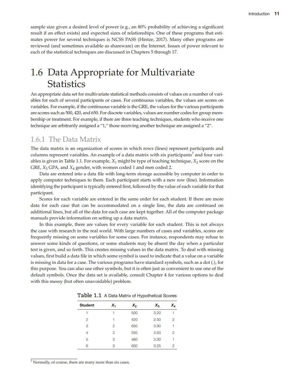
Th e d a ta ma t r ix is an organiza ti on of sco res in which rows (li n es) rep resen t pa r ti cipan ts a nd co lumns represent vari ab les. An examp le of a da ta m atrix w i th s ix pa rticipants 7 a nd fo ur va r ia b les is given in Tab le 1.1. For e xamp le, X1 migh t be t ype of teaching tech niqu e, X2 sco re o n t h e G RE, X3 GPA, and X4 gend er, wi th women coded 1 and men coded 2.
Data are en tered into a da ta fi le w i th long- term s torage accessible by comp u ter in ord er to a p p ly co mp u ter techniqu es to them. Each participant s tarts with a new row (lin e). Info rma tion id entifying the p a r ticipan t is t ypica lly entered fi rs t, foll owed b y the valu e of each variab le for tha t participant.
Scores for each variab le a re e n te red in the same o r de r fo r each s tu den t If there a re more da ta fo r each case tha t can be accommoda te d on a single line, th e d a ta a re con tinu ed on ad d i tional lines, b u t a ll of the d a ta fo r each case are kept toge the r. All of the co mpu te r package m anuals p r ovid e infor ma ti on o n setting up a da ta ma trix.
1n this examp le, th e re a re values fo r ever y va r iab le fo r each s tu den t. This is n o t a lways the case w i th research in t h e rea l worl d. Wi th l arge n umbers of cases and variab les, scores are frequ entl y missin g on so m e variab l es for so me cases. For instance, respondents may refuse to answe r some k inds o f ques ti ons, or some s tu den ts may be absen t the day when a parti cu l a r tes t is g i ven, a n d so fo r th . This creates missing va l ues in the da ta m atrix. To dea l w ith missing valu es, firs t b uil d a d a ta file in which some sy mbo l is u sed to ind icate tha t a va lu e o n a variable is missin g in d a ta for a case. The va r io us p r ograms have standard symbols, s u ch as a dot (.), fo r this p u rpose. You can also use other sy mbo ls, bu t it is o ften just as con veni en t to u se one o f th e defa ult symbols. O n ce th e d ata se t is avai lable, consu l t Cha p ter 4 for va r iou s o pti on s to d eal w i th this messy (b u t often u n avoid able) p rob lem.
Table 1. 1 A Data M atrix of Hypoth et ical Sc ores
Tabl e 1. 2 C orrelat ion M at rix fo r Part of Hy pot het ical Data f or Tab le 1.1
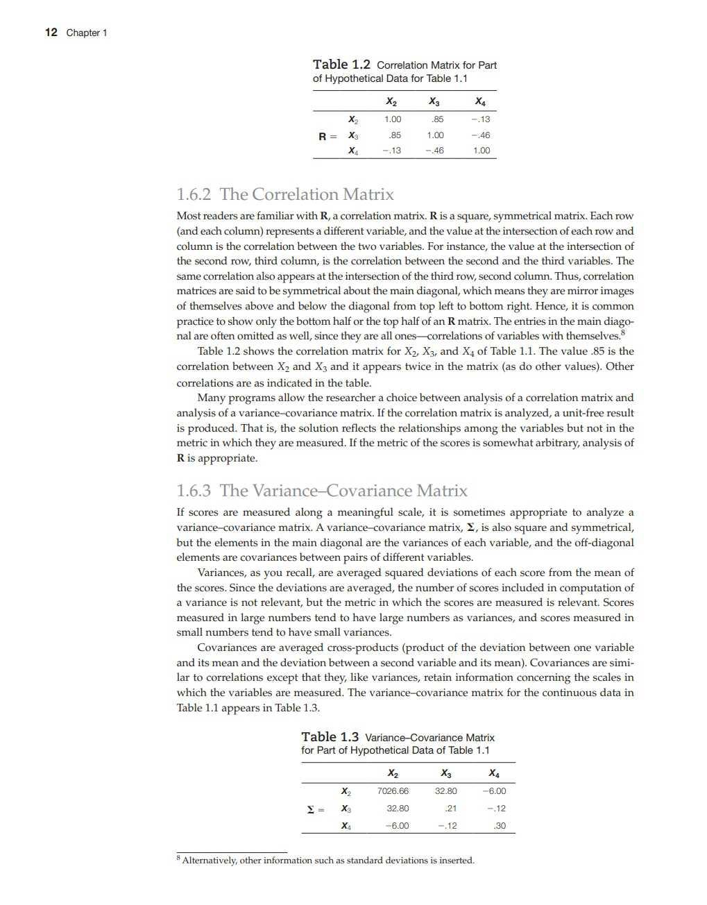
1.6.2 The Correlation Matrix
Mos t readers are familiar with R, a cor rel a tion matrix. R is a squ are, symmetrical ma trix. Each row (and each co lumn) rep resen ts a differen t variable, and the valu e at the intersection o f each r ow and column is the correlation b etween the t wo variables. For ins tance, the valu e a t the in tersec ti on of the second row, third column, is the co rrela ti on b etween the second and the third variab les. The sam e co rrel a ti on also appears a t the intersecti on of the third row, second column Thu s, cor rela tion ma trices are said to be symme trical abo u t the main d iagonal, which means they are mirror images o f themselves above and below the d iagonal from top left to bo ttom rig ht. Hence, it is common p racti ce to show only the bo tto m half or the top h alf o f an R ma trix The entries in the main d iagonal are often o mi tted as well , since they are all on es-cor rela tions of variab les with thernselves.8
Ta b le 1.2 shows the co rrelation matr ix for X2- X3 , and X4 of Table 1. 1. The va l ue .85 is the co rre lation between X2 and X3 a nd i t app ears tw ice in th e ma t r ix (as d o o the r valu es). Other co rre lations are as in d icated in the table.
Many p rograms a ll ow the resea rch er a choice between ana l ysis o f a corre lation ma trix and analysis of a variance-covari ance ma tr ix. If t h e co rrel ation matr ix is analyzed, a uni t-free resu lt is p rod u ced. Tha t is, the sol u ti on refl ects th e rel a ti on s h ips among the va r iab les b u t no t in the m etric in which th ey are measu red. If the metric o f the scores is somewha t a r b i tra r y, analysis of R is approp ria te.
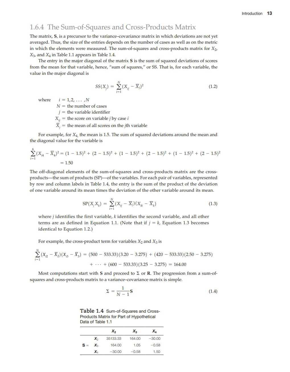
1.6.3 The Variance-Cov ariance Matrix
If sco res a re measu red along a meaningful scale, i t is so m etimes appropr ia te to ana lyze a var iance-covarian ce ma tri x . A variance-covari ance m a trix, l: , is also squ are a nd symme trica l, but the elemen ts in the ma in diagonal a re the vari ances of each va riable, and the o ff-diagon a l e lements are covari ances between pairs of differen t va riab les.
Var ian ces, as you reca ll , are averaged squ a red dev ia ti on s of each score fr o m the mean of the scores. Since the dev i ations are averaged , the n umbe r o f scores inclu ded in comp u tation of a va riance is not re levan t, bu t the m etric in w hi ch the sco res a re measu red is re levant. Scores m easured in la rge numbers tend to h ave la rge n umbers as va riances, a n d sco res measured in small n umbers tend to have small vari ances.
Cova riances are averaged cross-p roducts (p roduct o f th e d evia ti on b e t ween on e va riable and i ts m ean and th e dev iati on between a second va r iab le a n d i ts mean). Covarian ces a re similar to correla ti ons excep t tha t th ey, l i ke varia n ces, re tain infor ma ti on conce rnin g the scales in which the variables are measured. The var iance-cova r iance ma trix fo r the con tin uous da ta in Ta b le 1.1 appears in Ta b le 1.3.
T ab l e 1 .3 Varian c ErCovarianc e M atrix for Part of Hypo th et ical Data of Ta ble 1 1
x2 X3 x
x2 7026 66 32.80 - 6.00
l: = X3 32 80 .2 1 - 12 x. - 6.00 - .12 .30 8
1.6.4 The Sum-o f-Squares and Cross-P rod uc t s Matrix
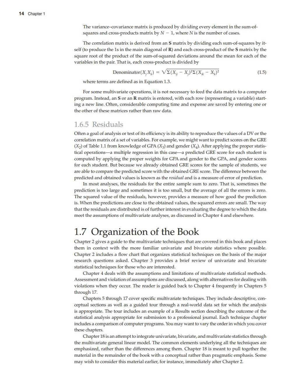
Th e ma trix, S, is a precursor to the va riance-cova riance ma tr ix in w h ich devia ti ons are n o t yet averaged. Thu s, the s ize of the entries depen ds on the number of cases as well as o n the metric in which the e lements were measured. The s um -of-s quares a n d cross-p r od u cts ma tr ix fo r Xz, X3 , and X4 in Table 1.1 appea rs in Table 1.4.
Th e en tr y in the majo r diagonal of the ma trix S is th e s um of squ ared dev iations o f scores fr om th e mean fo r tha t variab le, hence, "sum of squares," or SS. Th a t is, fo r each va r iab le, th e valu e in the major d i agona l is
where i = 1,2, ,N
N = the n u mb e r of cases
j = the variab le iden tifier
X1i = th e score on variab le j by case i
Xi = th e mean of a ll scores on the j th var iab le
Fo r example, fo r X4, th e mean is 1.5. The sum of squ ared dev iations a round th e mean a n d the diagon a l valu e for the va r iable is
6 2, ( Xi4 - X4 ) 2 = {1 - 1.5 ) 2 + {2 - 1.5)2 + {1 - 1.5) 2 + {2 - 1.5)2 + {1 - 1.5) 2 + {2 - 1.5) 2 = 1.50
The off-diagona l elements o f the sum-o f-squ a res and cross-products ma t r i x are th e c r ossprod u c ts- t h e sum o f products (SP)-o f the var iab les. For each pa ir of vari ab l es, rep resented by row and co lu mn labels in Tab le 1.4, the entry is the s u m of t h e p rod u c t o f the deviation of o n e va ri ab le aroun d its mean ti mes the dev i a ti on of the o th er variab le a round i ts mean. N
SP{X1 Xk) = 2, ( X1i- Xi )( X1k - X k) J=l (1.3)
w h e re j iden tifies t he firs t va r iab le, k iden ti fies t he second var i able, and all othe r terms a re as defin ed in Equa t ion 1.1. (Note tha t if j = k, Equation 1.3 becomes ident ica l to Equ at ion 1.2.)
Fo r examp le, the cross-p roduct term fo r va r iables X2 and X3 is
N 2, {X,1 - X2 ){ X13 - X3 ) = {500 - 533.33){3.20 - 3.275 ) + {420 - 533.33 ){ 2.50 - 3.275) + + {600 - 533.33 ){3.25 - 3.275) = 164.00
Most compu ta ti ons start wi th S and proceed to o r R. The progressi on from a s u m-ofsqu ares and cross -produc ts ma tr ix to a varian ce-covarian ce ma tr ix is s imple.
!. = --s N - 1
Table 1.4 Sum-of -Sq uares and CrossProd ucts Matri x f or Part of Hypothet ic al
Data of Tab le 1.1
(1.4)
Th e variance-covariance ma t rix is pro d u ced b y d i vi din g eve r y element in the s u m -ofsqu ares and cross-p roducts matr ix by N - 1, whe re N is the n umbe r of cases.
The correla ti on ma tr ix is der ived from a n S m atrix by d iv i ding each sum-of-squ ares by i tself (to prod u ce the 1s in the main d iagona l o f R ) and each cross-p roduct of the S m atrix b y t h e squ are r oo t o f th e produc t of the s um-of-squ a r ed dev iati on s a r ound the m ean fo r each of the var iab l es in the p a ir Tha t is, each cr oss-pr od u ct is d i vi ded by
D enominato r (X1 Xk) = Y!:(X;i- Xi ) 2 '£(X;k - Xk)2
where terms are defined as in Equ a ti on 1.3.
(1.5)
Fo r so m e m ul ti va r iate ope rations, i t is not necessary to feed the da ta m a trix to a comp uter p r ogr a m Instead , an S o r an R ma trix is en te r ed, w ith each r ow (repr esent ing a variab le) s ta rtin g a new line. Often, consid erab le com p u t ing t ime and expense a r e saved by ent e ring one or the o the r o f these m a trices rather than raw d a t a.
1.6.5 Residua ls
O ften a goa l of ana lysis o r test of i ts effi ciency is i ts ab ility t o r epr oduce the values of a D V o r the correla ti on matrix of a se t of vari abl es. Fo r exa mp le, we migh t wan t to p r ed ic t scor es on the GRE (X2 ) of Table 1. 1 fro m kn ow led ge of G PA (X3 ) and gen der (X4). After app ly ing the p roper sta tistica l oper a tions- a mu lt ip le r egression in this case- a p red icted GRE scor e fo r each s tu dent is computed b y applyin g the p roper weights fo r GPA and gender to the GPA, and gender scores fo r each stu d ent. Bu t b ecause we a lready ob tained G RE sco res fo r the sam p le of stu d en ts, we a r e able to compa r e the p red icted score with the ob t ained G RE score. The d ifference between t h e p r ed icted and ob t ained values is known as the residual and is a measur e o f error of p red iction. In m ost ana lyses, the residu als for th e ent ire sample su m to zero. Th a t is, som e tim es t h e p r ed icti on is too large and so me tim es it is too sma ll , b u t the aver age of a ll t h e err ors is zer o. The squ a r ed valu e o f the resi d u als, however, p rov id es a measu re of how good th e p redic ti on is. When th e p redic ti ons a re close to the ob tained va lues, th e squa r ed erro rs are sma ll . The way tha t the resi d u als a re d is trib u ted is of fu r the r interest in eva l ua t ing th e degree t o w h ich the d ata m eet the assump ti on s o f mu l ti va ri ate a n a lyses, as d iscu ssed in C h apter 4 and e lsewher e.
1. 7 Organ iza tion of the Book
Chap ter 2 gives a gui de t o the m u l ti va ria t e t echniqu es th at are cove red in this book and p l aces the m in con tex t wi th the m o r e famil iar u n i varia te an d b iva r iate statisti cs w h er e possib le. C hap ter 2 incl udes a fl ow chart tha t o r ganizes s tatis tical t echni ques on th e basis of the m ajor resea r ch q u esti on s ask ed. C h apter 3 provid es a br ief review of u n ivari ate a n d b i va r ia t e s ta tistical techni ques fo r those who are interest ed.
C hap te r 4 deals w i t h th e assump ti ons a n d li mi ta ti on s of m u lti var ia te s tatistical methods. Assessm ent and viola ti on of assu mpti on s ar e d iscu ssed, alon g w i th alterna ti ves for dealing w i th viola ti ons when th ey occur The reader is gui ded b ack to Chap te r 4 freq u en tly in Chapte r s 5 through 17.
C hap ters 5 throu gh 17 cover specific mul tivaria te techni qu es. They include d escr ip tive, conceptual section s as well as a guid ed tour throu gh a real-world data set fo r which the anal ysis is appropria t e. The t o ur includ es an exam p le of a Res ul ts sec ti on describ ing the outcome of the s t atis tical anal ysis approp riate for submiss ion to a p rofessional journal. Ea ch technique chap ter includ es a com parison of com p u ter p rogr ams. Yo u m ay want t o vary the o rder in whi ch you cover these chapter s.
C hapter 18 is an attem pt to integra te uni va riate, biva r ia te, and mul ti va riate statistics through the m u l tivari a te gener al linea r m odel. The co mmon e lemen ts u nderl ying all the techni ques are emph asized, r ather than the differences am ong them . Chapter 18 is m eant to p u ll togethe r the ma te ri al in the rem a in der of the b ook with a conceptu al r ather than pragma ti c e mp hasis. Som e may w ish t o con s id er this m ater ial earli er, for inst ance, immedi a tel y after C h a p te r 2.