Where can buy Remote sensing of the environment : an earth resource perspective 2nd ed, pearson new
Visit to download the full and correct content document: https://ebookmass.com/product/remote-sensing-of-the-environment-an-earth-resourc e-perspective-2nd-ed-pearson-new-international-edition-edition-jensen/
More products digital (pdf, epub, mobi) instant download maybe you interests ...
All rights reserved. No part of this publication may be reproduced, stored in a retrieval system, or transmitted in any form or by any means, electronic, mechanical, photocopying, recording or otherwise, without either the prior written permission of the publisher or a licence permitting restricted copying in the United Kingdom issued by the Copyright Licensing Agency Ltd, Saffron House, 6–10 Kirby Street, London EC1N 8TS.
All trademarks used herein are the property of their respective owners. The use of any trademark in this text does not vest in the author or publisher any trademark ownership rights in such trademarks, nor does the use of such trademarks imply any affiliation with or endorsement of this book by such owners.
ISBN 10: 1-292-02170-5
ISBN 13: 978-1-292-02170-6
British Library Cataloguing-in-Publication Data
A catalogue record for this book is available from the British Library
14. In Situ Spectral Reflectance Measurement
John R. Jensen
Appendix—Sources of Remote Sensing Information 601
John R. Jensen
Remote Sensing of the Environment
Scientists observe nature, make measurements, and then attempt to accept or reject hypotheses concerning these phenomena. The data collection may take place directly in the field (referred to as in situ or in-place data collection), or at some remote distance from the subject matter (referred to as remote sensing of the environment).
In situ Data Collection
One form of in situ data collection involves the scientist going out in the field and questioning the phenomena of interest. For example, a census enumerator may go door to door, asking people questions about their age, sex, education, income, etc. These data are recorded and used to document the demographic characteristics of the population.
Conversely, a scientist may use a transducer or other in situ measurement device at the study site to make measurements. Transducers are usually placed in direct physical contact with the object of interest. Many different types of transducers are available. For example, a scientist could use a thermometer to measure the temperature of the air, soil, or water; an anemometer to measure wind speed; or a psychrometer to measure air humidity. The data recorded by the transducers may be an analog electrical signal with voltage variations related to the intensity of the property being measured. Often these analog signals are transformed into digital values using analog-to-digital (Ato-D) conversion procedures. In situ data collection using transducers relieves the scientist of monotonous data collection often in inclement weather. Also, the scientist can distribute the transducers at important geographic locations throughout the study area, allowing the same type of measurement to be obtained at many locations at the same time. Sometimes data from the transducers are telemetered electronically to a central collection point for rapid evaluation and archiving (e.g., Teillet et al., 2002).
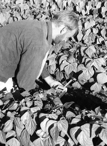
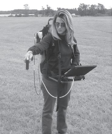
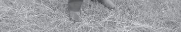
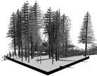
Two examples of in situ data collection are demonstrated in Figure 1. Leafarea-index (LAI) measurements are being collected by a scientist at a study site using a handheld ceptometer in Figure 1a. Spectral reflectance measurements of vegetation are being obtained at a study site using a handheld spectroradiometer in Figure 1b. LAI and spectral reflectance measurements obtained in the field may be used to calibrate LAI and spectral reflectance measurements collected by a remote sensing system located on an aircraft or satellite (Jensen et al., 2005).
a. Leaf-area-index (LAI) measurement using a ceptometer.
b. Spectral reflectance measurement using a spectroradiometer. radiometer in backpack detector personal computer
Figure 1 In situ (in-place) data are collected in the field. a) A scientist is collecting leaf-area-index (LAI) measurements of soybeans (Glycine max L. Merrill) using a ceptometer that measures the number of “sunflecks” that pass through the vegetation canopy. The measurements are made just above the canopy and on the ground below the canopy. The in situ LAI measurements may be used to calibrate LAI estimates derived from remote sensor data. b) Spectral reflectance measurements from vegetation are being collected using a spectroradiometer located approximately 1 m above the canopy. The in situ spectral reflectance measurements may be used to calibrate the spectral reflectance measurements obtained from a remote sensing system.
Data collection by scientists in the field or by instruments placed in the field provide much of the data for physical, biological, and social science research. However, it is important to remember that no matter how careful the scientist is, error may be introduced during the in situ data-collection process. First, the scientist in the field can be intrusive. This means that unless great care is exercised, the scientist can actually change the characteristics of the phenomenon being measured during the data-collection process. For example, a scientist could lean out of a boat to obtain a surface-water sample from a lake. Unfortunately, the movement of the boat into the area may have stirred up the water column in the vicinity of the water sample, resulting in an unrepresentative, or biased, sample. Similarly, a scientist collecting a spectral reflectance reading could inadvertently step on the sample site, disturbing the vegetation canopy prior to data collection.
Scientists may also collect data in the field using biased procedures. This introduces method-produced error. It could
involve the use of a biased sampling design or the systematic, improper use of a piece of equipment. Finally, the in situ data-collection measurement device may be calibrated incorrectly. This can result in serious measurement error.
Intrusive in situ data collection, coupled with human method-produced error and measurement-device miscalibration, all contribute to in situ data-collection error. Therefore, it is a misnomer to refer to in situ data as ground truth data. Instead, we should simply refer to it as in situ ground reference data, acknowledging that it contains error.
Remote Sensing Data Collection
Fortunately, it is also possible to collect information about an object or geographic area from a distant vantage point using remote sensing instruments (Figure 2). Remote sens-
Remote Sensing of the Environment
Remote Sensing Measurement
Orbital platform
Suborbital platform
Suborbital platform
Remote sensing instrument
H altitude above ground level (AGL)
β instantaneousfield-of-view (IFOV) of the sensor system
Object, area, or materials within the ground-projected IFOV
diameter of the ground-projected IFOV
Figure 2 A remote sensing instrument collects information about an object or phenomenon within the instantaneous-field-of-view (IFOV) of the sensor system without being in direct physical contact with it. The remote sensing instrument may be located just a few meters above the ground and/or onboard an aircraft or satellite platform.
ing data collection was originally performed using cameras mounted in suborbital aircraft. Photogrammetry was defined in the early editions of the Manual of Photogrammetry as:
the art or science of obtaining reliable measurement by means of photography (American Society of Photogrammetry, 1952; 1966).
Photographic interpretation is defined as:
the act of examining photographic images for the purpose of identifying objects and judging their significance (Colwell, 1960).
Remote sensing was formally defined by the American Society for Photogrammetry and Remote Sensing (ASPRS) as:
the measurement or acquisition of information of some property of an object or phenomenon, by a recording device that is not in physical or intimate contact with the object or phenomenon under study (Colwell, 1983).
In 1988, ASPRS adopted a combined definition of photogrammetry and remote sensing:
Photogrammetry and remote sensing are the art, science, and technology of obtaining reliable information about physical objects and the environment, through the process of recording, measuring and interpreting imagery and digital representations of energy patterns derived from non-contact sensor systems (Colwell, 1997).
But where did the term remote sensing come from? The actual coining of the term goes back to an unpublished paper in the early 1960s by the staff of the Office of Naval Research Geography Branch (Pruitt, 1979; Fussell et al., 1986). Evelyn L. Pruitt was the author of the paper. She was assisted by staff member Walter H. Bailey. Aerial photo interpretation had become very important in World War II. The space age was just getting under way with the 1957 launch of Sputnik (U.S.S.R.), the 1958 launch of Explorer 1 (U.S.), and the collection of photography from the then secret CORONA program initiated in 1960 (Table 1). In addition, the Geography Branch of ONR was expanding its research using instruments other than cameras (e.g., scanners, radiometers) and into regions of the electromagnetic spectrum beyond the visible and near-infrared regions (e.g., thermal infrared, microwave). Thus, in the late 1950s it had become apparent that the prefix “photo” was being stretched too far in view of the fact that the root word, photography,
literally means “to write with [visible] light” (Colwell, 1997). Evelyn Pruitt (1979) wrote:
The whole field was in flux and it was difficult for the Geography Program to know which way to move. It was finally decided in 1960 to take the problem to the Advisory Committee. Walter H. Bailey and I pondered a long time on how to present the situation and on what to call the broader field that we felt should be encompassed in a program to replace the aerial photointerpretation project. The term ‘photograph’ was too limited because it did not cover the regions in the electromagnetic spectrum beyond the ‘visible’ range, and it was in these nonvisible frequencies that the future of interpretation seemed to lie. ‘Aerial’ was also too limited in view of the potential for seeing the Earth from space.
The term remote sensing was promoted in a series of symposia sponsored by ONR at the Willow Run Laboratories of the University of Michigan in conjunction with the National Research Council throughout the 1960s and early 1970s, and has been in use ever since (Estes and Jensen, 1998).
Maximal/Minimal Definitions
Numerous other definitions of remote sensing have been proposed. In fact, Colwell (1984) suggests that “one measure of the newness of a science, or of the rapidity with which it is developing is to be found in the preoccupation of its scientists with matters of terminology.” Some have proposed an all-encompassing maximal definition:
Remote sensing is the acquiring of data about an object without touching it.
Such a definition is short, simple, general, and memorable. Unfortunately, it excludes little from the province of remote sensing (Fussell et al., 1986). It encompasses virtually all remote sensing devices, including cameras, optical-mechanical scanners, linear and area arrays, lasers, radar systems, sonar, seismographs, gravimeters, magnetometers, and scintillation counters.
Others have suggested a more focused, minimal definition of remote sensing that adds qualifier after qualifier in an attempt to make certain that only legitimate functions are included in the term’s definition. For example:
Remote sensing is the noncontact recording of information from the ultraviolet, visible, infrared,
and microwave regions of the electromagnetic spectrum by means of instruments such as cameras, scanners, lasers, linear arrays, and/or area arrays located on platforms such as aircraft or spacecraft, and the analysis of acquired information by means of visual and digital image processing.
Robert Green at NASA’s Jet Propulsion Lab (JPL) suggests that the term remote measurement might be used instead of remote sensing because data obtained using the new hyperspectral remote sensing systems are so accurate (Robbins, 1999). Each of the definitions are correct in an appropriate context. It is useful to briefly discuss components of these remote sensing definitions.
Remote Sensing: Art and/or Science?
Science: A science is defined as a broad field of human knowledge concerned with facts held together by principles (rules). Scientists discover and test facts and principles by the scientific method, an orderly system of solving problems. Scientists generally feel that any subject that humans can study by using the scientific method and other special rules of thinking may be called a science. The sciences include 1) mathematics and logic, 2) physical sciences, such as physics and chemistry, 3) biological sciences, such as botany and zoology, and 4) the social sciences, such as geography, sociology, and anthropology (Figure 3). Interestingly, some persons do not consider mathematics and logic to be sciences. But the fields of knowledge associated with mathematics and logic are such valuable tools for science that we cannot ignore them. The human race’s earliest questions were concerned with “how many” and “what belonged together.” They struggled to count, to classify, to think systematically, and to describe exactly. In many respects, the state of development of a science is indicated by the use it makes of mathematics. A science seems to begin with simple mathematics to measure, then works toward more complex mathematics to explain.
Remote sensing is a tool or technique similar to mathematics. Using sophisticated sensors to measure the amount of electromagnetic energy exiting an object or geographic area from a distance and then extracting valuable information from the data using mathematically and statistically based algorithms is a scientific activity (Fussell et al., 1986). Remote sensing functions in harmony with other geographic information sciences (often referred to as GIScience), including cartography, surveying, and geographic information systems (GIS) (Curran, 1987; Clarke, 2001; Jensen, 2005). Dahlberg and Jensen (1986) and Fisher and Lindenberg (1989) suggested a model where there is interaction
Remote
Sensing of the Environment
Figure 3 Interaction model depicting the relationship of the geographic information sciences (remote sensing, geographic information systems, cartography, and surveying) as they relate to mathematics and logic and the physical, biological, and social sciences.
between remote sensing, cartography, surveying, and GIS, where no subdiscipline dominates and all are recognized as having unique yet overlapping areas of knowledge and intellectual activity as they are used in physical, biological, and social science research (Figure 3).
The theory of science suggests that scientific disciplines go through four classic developmental stages. Wolter (1975) suggested that the growth of a scientific discipline, such as remote sensing, that has its own techniques, methodologies, and intellectual orientation seems to follow the sigmoid or logistic curve illustrated in Figure 4. The growth stages of a scientific field are: Stage 1 — a preliminary growth period with small increments of literature; Stage 2 — a period of exponential growth when the number of publications doubles at regular intervals; Stage 3 — a period when the rate of growth begins to decline but annual increments remain constant; and Stage 4 — a final period when the rate of growth approaches zero. The characteristics of a scholarly field during each of the stages may be briefly described as follows: Stage 1 — little or no social organization; Stage 2 — groups of collaborators and existence of invisible colleges, often in the form of ad hoc institutes, research units, etc.; Stage 3 — increasing specialization and increasing controversy; and Stage 4 — decline in membership in both collaborators and invisible colleges.
Developmental Stages of a Scientific Discipline
Stage 1Stage 2Stage 3Stage 4
Figure 4 The developmental stages of a scientific discipline (Wolter, 1975; Jensen and Dahlberg, 1983).
Using this logic, it may be suggested that remote sensing is in Stage 2 of a scientific field, experiencing exponential growth since the mid-1960s with the number of publications doubling at regular intervals (Colwell, 1983; Cracknell and Hayes, 1993; Jensen, 2005). Empirical evidence is presented in Table 1, including: 1) the organization of many specialized institutes and centers of excellence associated with remote sensing, 2) the organization of numerous professional societies devoted to remote sensing research, 3) the publication of numerous new scholarly remote sensing journals, 4) significant technological advancement such as improved sensor systems and methods of image analysis, and 5) intense self-examination (e.g., Dehqanzada and Florini, 2000). We may be approaching Stage 3 with increasing specialization and theoretical controversy. However, the rate of growth of remote sensing has not begun to decline. In fact, there has been a tremendous surge in the numbers of persons specializing in remote sensing and commercial firms using remote sensing during the 1990s and early 2000s (Davis, 1999; ASPRS, 2004). Significant improvements in the spatial resolution of satellite remote sensing (e.g., more useful 1 × 1 m panchromatic data) has brought even more social science GIS practitioners into the fold. Hundreds of new peer-reviewed remote sensing research articles are published every month.
Art: The process of visual photo or image interpretation brings to bear not only scientific knowledge, but all of the background that a person has obtained through his or her lifetime. Such learning cannot be measured, programmed, or completely understood. The synergism of combining scientific knowledge with real-world analyst experience allows the interpreter to develop heuristic rules of thumb to extract
Remote Sensing of the Environment
Table 1. Major milestones in remote sensing.
1600 and 1700s
1687 - Sir Isaac Newton’s Principia summarizes basic laws of mechanics
1800s
1826 - Joseph Nicephore Niepce takes first photograph
1839 - Louis M. Daguerre invents positive print daguerrotype photography
1839 - William Henry Fox Talbot invents Calotype negative/positive process
1855 - James Clerk Maxwell postulates additive color theory
1858 - Gaspard Felix Tournachon takes aerial photograph from a balloon
1860s - James Clerk Maxwell puts forth electromagnetic wave theory
1867 - The term photogrammetry is used in a published work
1873 - Herman Vogel extends sensitivity of emulsion dyes to longer wavelengths, paving the way for near-infrared photography
1900
1903 - Airplane invented by Wright Brothers (Dec 17)
1903 - Alfred Maul patents a camera to obtain photographs from a rocket
1910s
1910 - International Society for Photogrammetry (ISP) founded in Austria
1913 - First International Congress of ISP in Vienna 1914 to 1918 - World War I photo-reconnaissance
1920s
1920 to 1930 - Increase civilian photointerpretation and photogrammetry
1926 - Robert Goddard launches liquid-powered rocket (Mar 16)
1930s
1934 - American Society of Photogrammetry (ASP) founded 1934 - Photogrammetric Engineering (ASP)
1938 - Photogrammetria (ISP)
1939 to 1945 - World War II photo-reconnaissance advances
1940s
1940s - RADAR invented
1940s - Jet aircraft invented by Germany
1942 - Kodak patents first false-color infrared film
1942 - Launch of German V-2 rocket by Wernher VonBraun (Oct 3)
1950s
1950s - Thermal infrared remote sensing invented by military
1950 - 1953 Korean War aerial reconnaissance
1953 - Photogrammetric Record (Photogrammetric Society, U.K.)
1954 - Westinghouse, Inc. develops side-looking airborne radar system
1955 to 1956 - U.S. Genetrix balloon reconnaissance program
1956 to 1960 - Central Intelligence Agency U-2 aerial reconnaissance program
1957 - Soviet Union launched Sputnik satellite (Oct 4)
1958 - United States launched Explorer 1 satellite (Jan 31)
1960s
1960s - Emphasis primarily on visual image processing
1960s - Michigan Willow Run Laboratory active — evolved into ERIM
1960s - First International Symposium on Remote Sensing of Environment at Ann Arbor, MI
1960s - Purdue Laboratory for Agricultural Remote Sensing (LARS) active
1960s - Forestry Remote Sensing Lab at U.C. Berkeley (Robert Colwell)
1960s - ITC– Delft initiates photogrammetric education for foreign students
1960s - Digital image processing initiated at LARS, Berkeley, Kansas, ERIM
1960s - Declassification of radar and thermal infrared sensor systems
1960 - 1972 United States COEONA spy satellite program
1960 - Manual of Photo-interpretation (ASP)
1960 - Term remote sensing introduced by Evelyn Pruitt and other U. S. Office of Naval Research personnel
1961 - Yuri Gagarin becomes first human to travel in space
1961 - 1963 Mercury space program
1962 - Cuban Missile Crisis — U-2 photo-reconnaissance shown to the public
1964 - SR-71 discussed in President Lyndon Johnson press briefing
1965 to 1966 - Gemini space program
1965 - ISPRS Journal of Photogrammetry & Remote Sensing
1969 - Remote Sensing of Environment (Elsevier)
Table 1. continued
1970s
1970s, 80s - Possible to specialize in remote sensing at universities
1970s - Digital image processing comes of age
1970s - Remote sensing integrated with geographic information systems
2005 - Google Earth serves DigitalGlobe and Landsat TM data
2006 - ORBIMAGE purchases Space Imaging and changes name to GeoEye
Remote Sensing of the Environment
valuable information from the imagery. It is a fact that some image analysts are superior to other image analysts because they: 1) understand the scientific principles better, 2) are more widely traveled and have seen many landscape objects and geographic areas, and/or 3) they can synthesize scientific principles and real-world knowledge to reach logical and correct conclusions. Thus, remote sensing image interpretation is both an art and a science.
Information About an Object or Area
Sensors can obtain very specific information about an object (e.g., the diameter of an oak tree crown) or the geographic extent of a phenomenon (e.g., the polygonal boundary of an entire oak forest). The electromagnetic energy emitted or reflected from an object or geographic area is used as a surrogate for the actual property under investigation. The electromagnetic energy measurements must be turned into information using visual and/or digital image processing techniques.
The Instrument (Sensor)
Remote sensing is performed using an instrument, often referred to as a sensor. The majority of remote sensing instruments record EMR that travels at a velocity of 3 × 10⁸ m s–1 from the source, directly through the vacuum of space or indirectly by reflection or reradiation to the sensor. The EMR represents a very efficient high-speed communications link between the sensor and the remote phenomenon. In fact, we know of nothing that travels faster than the speed of light. Changes in the amount and properties of the EMR become, upon detection by the sensor, a valuable source of data for interpreting important properties of the phenomenon (e.g., temperature, color). Other types of force fields may be used in place of EMR, such as acoustic (sonar) waves (e.g., Dartnell and Gardner, 2004). However, the majority of remotely sensed data collected for Earth resource applications is the result of sensors that record electromagnetic energy.
Distance: How Far Is Remote?
Remote sensing occurs at a distance from the object or area of interest. Interestingly, there is no clear distinction about how great this distance should be. The intervening distance could be 1 cm, 1 m, 100 m, or more than 1 million m from the object or area of interest. Much of astronomy is based on remote sensing. In fact, many of the most innovative remote sensing systems and visual and digital image processing methods were originally developed for remote sensing extraterrestrial landscapes such as the moon, Mars, Io, Saturn, Jupiter, etc. This text, however, is concerned primarily with
remote sensing of the terrestrial Earth, using sensors that are placed on suborbital air-breathing aircraft or orbital satellite platforms placed in the vacuum of space.
Remote sensing and digital image processing techniques can also be used to analyze inner space. For example, an electron microscope can be used to obtain photographs of extremely small objects on the skin, in the eye, etc. An x-ray instrument is a remote sensing system where the skin and muscle are like the atmosphere that must be penetrated, and the interior bone or other matter is the object of interest.
Remote Sensing Advantages and Limitations
Remote sensing has several unique advantages as well as some limitations.
Advantages
Remote sensing is unobtrusive if the sensor is passively recording the electromagnetic energy reflected from or emitted by the phenomenon of interest. This is a very important consideration, as passive remote sensing does not disturb the object or area of interest.
Remote sensing devices are programmed to collect data systematically, such as within a single 9 × 9 in. frame of vertical aerial photography or a matrix (raster) of Landsat 5 Thematic Mapper data. This systematic data collection can remove the sampling bias introduced in some in situ investigations (e.g., Karaska et al., 2004).
Remote sensing science is also different from cartography or GIS because these sciences rely on data obtained by others. Remote sensing science can provide fundamental, new scientific information. Under controlled conditions, remote sensing can provide fundamental biophysical information, including x,y location; z elevation or depth; biomass; temperature; and moisture content. In this sense, remote sensing science is much like surveying, providing fundamental information that other sciences can use when conducting scientific investigations. However, unlike much of surveying, the remotely sensed data can be obtained systematically over very large geographic areas rather than just single-point observations. In fact, remote sensing–derived information is now critical to the successful modeling of numerous natural (e.g., water-supply estimation; eutrophication studies; nonpoint source pollution) and cultural (e.g., land-use conversion at the urban fringe; water-demand estimation; population estimation) processes (Walsh et al., 1999; Stow et al., 2003; Nemani et al., 2003; Karaska et al., 2004). A good
Remote Sensing of the Environment
example is the digital elevation model that is so important in many spatially-distributed GIS models (Clarke, 2001). Digital elevation models are now produced mainly from stereoscopic imagery, light detection and ranging (LIDAR) (e.g., Maune, 2001; Hodgson et al., 2003b; 2005), radio detection and ranging (RADAR) measurements, or interferometric synthetic aperture radar (IFSAR) imagery.
Limitations
Remote sensing science has limitations. Perhaps the greatest limitation is that it is often oversold. Remote sensing is not a panacea that will provide all the information needed to conduct physical, biological, or social science research. It simply provides some spatial, spectral, and temporal information of value in a manner that we hope is efficient and economical.
Human beings select the most appropriate remote sensing system to collect the data, specify the various resolutions of the remote sensor data, calibrate the sensor, select the platform that will carry the sensor, determine when the data will be collected, and specify how the data are processed. Human method-produced error may be introduced as the remote sensing instrument and mission parameters are specified.
Powerful active remote sensor systems that emit their own electromagnetic radiation (e.g., LIDAR, RADAR, SONAR) can be intrusive and affect the phenomenon being investigated. Additional research is required to determine how intrusive these active sensors can be.
Remote sensing instruments may become uncalibrated, resulting in uncalibrated remote sensor data. Finally, remote sensor data may be expensive to collect and analyze. Hopefully, the information extracted from the remote sensor data justifies the expense. Interestingly, the greatest expense in a typical remote sensing investigation is for well-trained image analysts, not remote sensor data.
The Remote Sensing Process
Scientists have been developing procedures for collecting and analyzing remotely sensed data for more than 150 years. The first photograph from an aerial platform (a tethered balloon) was obtained in 1858 by the Frenchman Gaspard Felix Tournachon (who called himself Nadar). Significant strides in aerial photography and other remote sensing data collection took place during World War I and II, the Korean Conflict, the Cuban Missile Crisis, the Vietnam War, the Gulf
War, the war in Bosnia, and the war on terrorism. Many of the accomplishments are summarized in Table 1. Basically, military contracts to commercial companies resulted in the development of sophisticated electrooptical multispectral remote sensing systems and thermal infrared and microwave (radar) sensor systems. While the majority of the remote sensing systems may have been initially developed for military reconnaissance applications, the systems are also heavily used for monitoring the Earth’s natural resources.
The remote sensing data-collection and analysis procedures used for Earth resource applications are often implemented in a systematic fashion that can be termed the remote sensing process. The procedures in the remote sensing process are summarized here and in Figure 5:
• The hypothesis to be tested is defined using a specific type of logic (e.g., inductive, deductive) and an appropriate processing model (e.g., deterministic, stochastic).
• In situ and collateral data necessary to calibrate the remote sensor data and/or judge its geometric, radiometric, and thematic characteristics are collected.
• Remote sensor data are collected passively or actively using analog or digital remote sensing instruments, ideally at the same time as the in situ data.
• In situ and remotely sensed data are processed using a) analog image processing, b) digital image processing, c) modeling, and d) n-dimensional visualization.
• Metadata, processing lineage, and the accuracy of the information are provided and the results communicated using images, graphs, statistical tables, GIS databases, Spatial Decision Support Systems (SDSS), etc.
It is useful to review the characteristics of these remote sensing process procedures.
Statement of the Problem
Sometimes the general public and even children look at aerial photography or other remote sensor data and extract useful information. They typically do this without a formal hypothesis in mind. More often than not, however, they interpret the imagery incorrectly because they do not understand the nature of the remote sensing system used to collect
Statement of the Problem
• Formulate Hypothesis (if appropriate)
• Select Appropriate Logic
- Inductive and/or
- Deductive
- Technological
• Select Appropriate Model
- Deterministic
- Empirical
- Knowledge-based
- Process-based
- Stochastic
The Remote Sensing Process
Data Collection
Data-to-Information Conversion
• In Situ Measurements
- Field (e.g., x,y,z from GPS, biomass, reflectance)
- Laboratory (e.g., reflectance, leaf area index)
• Collateral Data
- Digital elevation models
- Soil maps
- Surficial geology maps
- Population density, etc.
• Remote Sensing
- Passive analog
- Frame camera
- Videography
- Passive digital
- Frame camera
- Scanners
- Multispectral
- Hyperspectral
- Linear and area arrays
- Multispectral
- Hyperspectral
- Active
- Microwave (RADAR)
- Laser (LIDAR)
- Acoustic (SONAR)
• Analog (Visual) Image Processing
- Using the Elements of Image Interpretation
• Digital Image Processing
- Preprocessing
- Radiometric Correction
- Geometric Correction
- Enhancement
- Photogrammetric analysis
- Parametric, such as
- Maximum likelihood
- Nonparametric, such as
- Artificial neural networks
- Nonmetric, such as
- Expert systems
- Decision-tree classifiers
- Machine learning
- Hyperspectral analysis
- Change detection
- Modeling
- Spatial modeling using GIS data
- Scene modeling
- Scientific geovisualization
- 1, 2, 3, and n dimensions
• Hypothesis Testing
- Accept or reject hypothesis
Information Presentation
• Image Metadata
- Sources
- Processing lineage
• Accuracy Assessment
- Geometric
- Radiometric
- Thematic
- Change detection
• Analog and Digital
- Images
- Unrectified
- Orthoimages
- Orthophotomaps
- Thematic maps
- GIS databases
- Animations
- Simulations
• Statistics
- Univariate
- Multivariate
• Graphs
- 1, 2, and 3 dimensions
Figure 5 Scientists generally use the remote sensing process when extracting information from remotely sensed data.
the data or appreciate the vertical or oblique perspective of the terrain recorded in the imagery.
Scientists who use remote sensing, on the other hand, are usually trained in the scientific method—a way of thinking about problems and solving them. They use a formal plan that has at least five elements: 1) stating the problem, 2) forming the research hypothesis (i.e., a possible explanation), 3) observing and experimenting, 4) interpreting data, and 5) drawing conclusions. It is not necessary to follow this formal plan exactly.
The scientific method is normally used in conjunction with environmental models that are based on two primary types of logic:
•deductive logic
•inductive logic
Models based on deductive and/or inductive logic can be further subdivided according to whether they are processed deterministically or stochastically (Jensen, 2005). Some scientists extract new thematic information directly from remotely sensed imagery without ever explicitly using inductive or deductive logic. They are just interested in extracting information from the imagery using appropriate methods and technology. This technological approach is not as rigorous, but it is common in applied remote sensing. The approach can also generate new knowledge.
Remote sensing is used in both scientific (inductive and deductive) and technological approaches to obtain knowledge. There is debate as to how the different types of logic used in the remote sensing process yield new scientific knowledge (e.g., Fussell et al., 1986; Curran, 1987; Fisher and Lindenberg, 1989; Dobson, 1993; Skidmore, 2002).
Remote
Identification of In situ and Remote Sensing Data Requirements
If a hypothesis is formulated using inductive and/or deductive logic, a list of variables or observations are identified that will be used during the investigation. In situ observation and/or remote sensing may be used to collect information on the most important variables.
Scientists using remote sensing technology should be well trained in field and laboratory data-collection procedures. For example, if a scientist wants to map the surface temperature of a lake, it is usually necessary to collect some accurate empirical in situ lake-temperature measurements at the same time the remote sensor data are collected. The in situ observations may be used to 1) calibrate the remote sensor data, and/or 2) perform an unbiased accuracy assessment of the final results (Congalton and Green, 1998). Remote sensing textbooks provide some information on field and laboratory sampling techniques. The in situ sampling procedures, however, are learned best through formal courses in the sciences (e.g., chemistry, biology, forestry, soils, hydrology, meteorology). It is also important to know how to collect accurately socioeconomic and demographic information in urban environments based on training in human geography, sociology, etc.
Most in situ data are now collected in conjunction with global positioning system (GPS) x, y, z data (Jensen and Cowen, 1999). Scientists should know how to collect the GPS data at each in situ data-collection station and how to perform differential correction to obtain accurate x, y, z coordinates (Rizos, 2002).
Collateral Data Requirements
Many times collateral data (often called ancillary data), such as digital elevation models, soil maps, geology maps, political boundary files, and block population statistics, are of value in the remote sensing process. Ideally, the spatial collateral data reside in a GIS (Clarke, 2001).
Remote Sensing Data Requirements
Once we have a list of variables, it is useful to determine which of them can be remotely sensed. Remote sensing can provide information on two different classes of variables: biophysical and hybrid
Biophysical Variables: Some biophysical variables can be measured directly by a remote sensing system. This means
that the remotely sensed data can provide fundamental biological and/or physical (biophysical) information directly, generally without having to use other surrogate or ancillary data. For example, a thermal infrared remote sensing system can record the apparent temperature of a rock outcrop by measuring the radiant energy exiting its surface. Similarly, it is possible to conduct remote sensing in a very specific region of the spectrum and identify the amount of water vapor in the atmosphere. It is also possible to measure soil moisture content directly using microwave remote sensing techniques (Engman, 2000). NASA’s Moderate Resolution Imaging Spectrometer (MODIS) can be used to measure absorbed photosynthetically active radiation (APAR) and leaf area index (LAI). The precise x, y location, and height (z) of an object can be extracted directly from stereoscopic aerial photography, overlapping satellite imagery (e.g., SPOT), light detection and ranging (LIDAR) data, or interferometric synthetic aperture radar (IFSAR) imagery.
Table 2 is a list of selected biophysical variables that can be remotely sensed and useful sensors to acquire the data. Great strides have been made in remotely sensing many of these biophysical variables. They are important to the national and international effort under way to model the global environment (Jensen et al., 2002; Asrar, 2004).
Hybrid Variables: The second general group of variables that can be remotely sensed include hybrid variables, created by systematically analyzing more than one biophysical variable. For example, by remotely sensing a plant’s chlorophyll absorption characteristics, temperature, and moisture content, it might be possible to model these data to detect vegetation stress, a hybrid variable. The variety of hybrid variables is large; consequently, no attempt is made to identify them. It is important to point out, however, that nominalscale land use and land cover are hybrid variables. For example, the land cover of a particular area on an image may be derived by evaluating several of the fundamental biophysical variables at one time [e.g., object location (x, y), height (z), tone and/or color, biomass, and perhaps temperature]. So much attention has been placed on remotely sensing this hybrid nominal-scale variable that the interval- or ratio-scaled biophysical variables were largely neglected until the mid-1980s. Nominal-scale land-use and land-cover mapping are important capabilities of remote sensing technology and should not be minimized. Many social and physical scientists routinely use such data in their research. However, there is now a dramatic increase in the extraction of interval- and ratio-scaled biophysical data that are incor-
Remote Sensing of the Environment
Table 2. Selected biophysical and hybrid variables and potential remote sensing systems used to obtain the information.
Biophysical
x, y, z Geodetic Control
VariablesPotential
x, y Location from Orthocorrected Imagery
z Topography/Bathymetry
- Digital Elevation Model (DEM)
- Digital Bathymetric Model (DBM)
Vegetation
- Pigments (e.g., chlorophyll a and b)
- Canopy structure and height
- Biomass derived from vegetation indices
- Leaf area index (LAI)
- Absorbed photosynthetically active radiation
- Evapotranspiration
Remote Sensing Systems
- Global Positioning Systems (GPS)
- Analog and digital stereoscopic aerial photography, Space Imaging IKONOS, DigitalGlobe QuickBird, Orbimage OrbView-3, French SPOT HRV, Landsat (Thematic Mapper, Enhanced TM+), Indian IRS-1CD, European ERS-1 and 2 microwave and ENVISAT MERIS, MODIS (Moderate Resolution Imaging Spectrometer), LIDAR, Canadian RADARSAT 1 and 2
- Color and CIR aerial photography, Landsat (TM, ETM+), SPOT, IKONOS, QuickBird, OrbView-3, ASTER, SeaWiFS, MODIS, airborne hyperspectral systems (e.g., AVIRIS, HyMap, CASI), AVHRR, GOES, bathymetric LIDAR, MISR, CERES, Hyperion, TOPEX/POSEIDON, MERIS
Remote Sensing of the Environment
Table 2. Selected biophysical and hybrid variables and potential remote sensing systems used to obtain the information.
Biophysical VariablesPotential Remote Sensing Systems
Snow and Sea Ice
- Extent and characteristics
Volcanic Effects
- Color and CIR aerial photography, AVHRR, GOES, Landsat (TM, ETM+), SPOT, SeaWiFS, IKONOS, QuickBird, ASTER, MODIS, MERIS, ERS-1 and 2, RADARSAT
- Temperature, gases- ASTER, MISR, Hyperion, MODIS, airborne hyperspectral systems
BRDF (bidirectional reflectance distribution function) - MISR, MODIS, CERES
Selected Hybrid VariablesPotential
Remote Sensing Systems
Land Use
- Commercial, residential, transportation, etc.
- Cadastral (property)
- Tax mapping
Land Cover
- Agriculture, forest, urban, etc.
Vegetation
- stress
- Very high spatial resolution panchromatic, color and /or CIR stereoscopic aerial photography, high spatial resolution satellite imagery (<1 x 1 m: IKONOS, QuickBird, OrbView-3), SPOT (2.5 m), LIDAR, high spatial resolution hyperspectral systems (e.g., AVIRIS, HyMap, CASI)
- Color and CIR aerial photography, Landsat (MSS, TM, ETM+), SPOT, ASTER, AVHRR, RADARSAT, IKONOS, QuickBird, OrbView-3, LIDAR, IFSAR, SeaWiFS, MODIS, MISR, MERIS, hyperspectral systems (e.g., AVIRIS, HyMap, CASI)
- Color and CIR aerial photography, Landsat (TM, ETM+), IKONOS, QuickBird, OrbView-3, AVHRR, SeaWiFS, MISR, MODIS, ASTER, MERIS, airborne hyperspectral systems (e.g., AVIRIS, HyMap, CASI)
porated into quantitative models that can accept spatially distributed information.
Remote Sensing Data Collection
Remotely sensed data are collected using passive or active remote sensing systems. Passive sensors record electromagnetic radiation that is reflected or emitted from the terrain (Shippert, 2004). For example, cameras and video recorders can be used to record visible and near-infrared energy reflected from the terrain. A multispectral scanner can be used to record the amount of thermal radiant flux exiting the terrain. Active sensors such as microwave (RADAR), LIDAR, or SONAR bathe the terrain in machine-made electromagnetic energy and then record the amount of radiant flux scattered back toward the sensor system.
Remote sensing systems collect analog (e.g., hard-copy aerial photography or video data) and/or digital data [e.g., a
matrix (raster) of brightness values obtained using a scanner, linear array, or area array]. A selected list of some of the most important remote sensing systems is presented in Table 3.
The amount of electromagnetic radiance, L (watts m-2 sr-1; watts per meter squared per steradian), recorded within the IFOV of an optical remote sensing system (e.g., a picture element in a digital image), is a function of: (1)
where
λ = wavelength (spectral response measured in various bands or at specific frequencies). Wavelength (λ) and frequency (υ) may be used interchangeably based on their relationship with the speed of light (c) where .
sx,y,z = x, y, z location of the pixel and its size (x, y);
Table 3. Selected remote sensing systems and their characteristics.
Remote Sensing of the Environment
t = temporal information, i.e., when, how long, and how often the data were acquired;
θ = set of angles that describe the geometric relationships between the radiation source (e.g., the Sun), the terrain target of interest (e.g., a corn field), and the remote sensing system;
P = polarization of back-scattered energy recorded by the sensor; and
Ω = radiometric resolution (precision) at which the data (e.g., reflected, emitted, or back-scattered radiation) are recorded by the remote sensing system.
It is useful to briefly review characteristics of the parameters associated with Equation 1 and how they influence the nature of the remote sensing data collected.
Spectral Information and Resolution
Most remote sensing investigations are based on developing a deterministic relationship (i.e., a model) between the amount of electromagnetic energy reflected, emitted, or back-scattered in specific bands or frequencies and the chemical, biological, and physical characteristics of the phenomena under investigation (e.g., a corn field canopy). Spectral resolution is the number and dimension (size) of specific wavelength intervals (referred to as bands or channels) in the electromagnetic spectrum to which a remote sensing instrument is sensitive.
Multispectral remote sensing systems record energy in multiple bands of the electromagnetic spectrum. For example, in the 1970s and early 1980s, the Landsat Multispectral Scan-ners (MSS) recorded remotely sensed data of much of the Earth that is still of significant value for change detection studies. The bandwidths of the four MSS bands are displayed in Figure 6a (band 1 = 500 – 600 nm; band 2 = 600 – 700 nm; band 3 = 700 – 800 nm; and band 4 = 800 – 1, 100 nm). The nominal size of a band may be large (i.e., coarse), as with the Landsat MSS near-infrared band 4 (800 – 1,100 nm) or relatively smaller (i.e., finer), as with the Landsat MSS band 3 (700 – 800 nm). Thus, Landsat MSS band 4 detectors recorded a relatively large range of reflected near-infrared radiant flux (300 nm wide) while the MSS band 3 detectors recorded a much reduced range of near-infrared radiant flux (100 nm wide).
The four multispectral bandwidths associated with the Positive Systems ADAR 5500 digital frame camera are shown
for comparative purposes (Figure 6a, c, and d). The camera’s bandwidths were refined to record information in more specific regions of the spectrum (band 1 = 450 – 515 nm; band 2 = 525 – 605 nm; band 3 = 640 – 690 nm; and band 4 = 750 – 900 nm). There are gaps between the spectral sensi-tivities of the detectors. Note that this digital camera system is also sensitive to reflected blue wavelength energy.
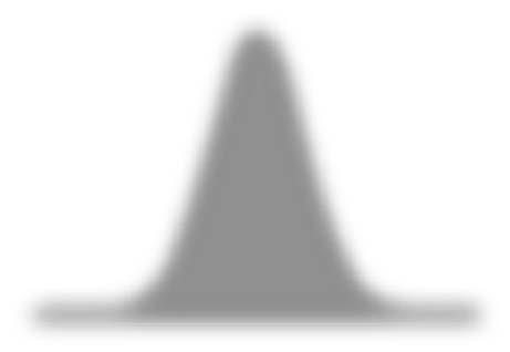
The aforementioned terminology is typically used to describe a sensor’s nominal spectral resolution. However, it is difficult to create a detector that has extremely sharp bandpass boundaries such as those shown in Figure 6a. Rather, the more precise method of stating bandwidth is to look at the typical Gaussian shape of the detector sensitivity, such as the example shown in Figure 6b. The analyst then determines the Full Width at Half Maximum (FWHM). In this hypothetical example, the Landsat MSS near-infrared band 3 under investigation is sens itive to energy between 700 and 800 nm.
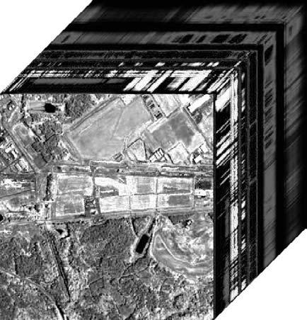
A hyperspectral remote sensing instrument typically acquires data in hundreds of spectral bands (Goetz, 2002). For example, the Airborne Visible and Infrared Imaging Spectrometer (AVIRIS) has 224 bands in the region from 400 to 2,500 nm spaced just 10 nm apart based on the FWHM criteria (Clark, 1999; NASA, 2006). An AVIRIS hyperspectral datacube of a portion of the Savannah River Site near Aiken, SC, is shown in Figure 7. Ultraspectral remote sensing involves data collection in many hundreds of bands.
Certain regions or spectral bands of the electromagnetic spectrum are optimal for obtaining information on biophysical parameters. The bands are normally selected to maximize the contrast between the object of interest and its background (i.e., object-to-background contrast). Careful selection of the spectral bands might improve the probability that the desired information will be extracted from the remote sensor data.
Spatial Information and Resolution
Most remote sensing studies record the spatial attributes of objects on the terrain. For example, each silver halide crystal in an analog aerial photograph and each picture element in a digital remote sensor image is located at a specific location in the image and associated with specific x,y coordinates on the ground. Once rectified to a standard map projection, the spatial information associated with each silver halide crystal or pixel is of significant value because it allows the remote sensing–derived information to be used with other spatial
Remote Sensing of the Environment
Figure 6 a) The spectral bandwidths of the four Landsat Multispectral Scanner (MSS) bands (green, red, and two near-infrared) compared with the bandwidths of an ADAR 5500 digital frame camera. b) The true spectral bandwidth is the width of the Gaussian-shaped spectral profile at Full Width at Half Maximum (FWHM) intensity (Clark, 1999). This example has a spectral bandwidth of 0.1 μm (100 nm) between 700 and 800 nm. c) If desired, it is possible to collect reflected energy in a single band of the electromagnetic spectrum (e.g., 750 – 900 nm). This is a 1 × 1 ft spatial resolution ADAR 5500 near-infrared image. d) Multispectral sensors collect data in multiple bands of the spectrum (images courtesy of Positive Systems, Inc.).
data in a GIS or spatial decision support system (Jensen et al., 2002).
There is a general relationship between the size of an object or area to be identified and the spatial resolution of the remote sensing system. Spatial resolution is a measure of the smallest angular or linear separation between two objects
that can be resolved by the remote sensing system. The spatial resolution of aerial photography may be measured by 1) placing calibrated, parallel black and white lines on tarps that are placed in the field, 2) obtaining aerial photography of the study area, and 3) computing the number of resolvable line pairs per millimeter in the photography. It is also possible to determine the spatial resolution of imagery by com-
Wavelength, μm
a. Nominal spectral resolution of the Landsat Multispectral Scanner and Positive Systems ADAR 5500 digital frame camera.
b. Precise bandpass measurement of a detector based on Full Width at Half Maximum (FWHM) criteria.
d. Multispectral remote sensing.
c. Single band of ADAR 5500 data.
Airborne Visible Infrared Imaging Spectrometer (AVIRIS) Datacube of the Savannah River Site near Aiken, SC
Near-infrared image on top of the datacube is just one of 224 bands at 10 nm nominal bandwidth acquired on July 26, 1999.
Figure 7 Hyperspectral imagery of an area on the Savannah River Site, SC obtained by NASA’s Airborne Visible/Infrared Imaging Spectrometer (AVIRIS). The nominal spatial resolution is 3.4 × 3.4 m. The atmosphere absorbs most of the electromagnetic energy near 1,400 and 1,900 nm, causing the dark bands in the hyperspectral datacube.
puting its modulation transfer function, which is beyond the scope of this text (Joseph, 2000).
Many satellite remote sensing systems use optics that have a constant instantaneous-field-of-view (IFOV) (Figure 2). Therefore, a sensor system’s nominal spatial resolution is defined as the dimension in meters (or feet) of the groundprojected IFOV where the diameter of the circle (D) on the ground is a function of the instantaneous-field-of-view (β) times the altitude (H) of the sensor above ground level (AGL) (Figure 2): (2)
D β H × =
Pixels are normally represented on computer screens and in hard-copy images as rectangles with length and width. Therefore, we typically describe a sensor system’s nominal
spatial resolution as being 10 × 10 m or 30 × 30 m. For example, DigitalGlobe’s QuickBird has a nominal spatial resolution of 61 × 61 cm for its panchromatic band and 2.44 × 2.44 m for the four multispectral bands. The Landsat 7 Enhanced Thematic Mapper Plus (ETM+) has a nominal spatial resolution of 15 × 15 m for its panchromatic band and 30 × 30 m for six of its multispectral bands. Generally, the smaller the nominal spatial resolution, the greater the spatial resolving power of the remote sensing system.
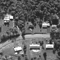
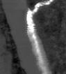
Figure 8 depicts digital camera imagery of an area in Mechanicsville, N.Y., at resolutions ranging from 0.5 × 0.5 m to 80 × 80 m. Note that there is not a significant difference in the interpretability of 0.5 × 0.5 m data, 1 × 1 m data, and even 2 × 2 m data. However, the urban information content decreases rapidly when using 5 × 5 m imagery and is practically useless for urban analysis at spatial resolutions larger than 10 × 10 m. This is the reason historical Landsat MSS data (79 × 79 m) are of little value for most urban applications (Jensen and Cowen, 1999; Jensen et al., 2002).
A useful heuristic rule of thumb is that in order to detect a feature, the nominal spatial resolution of the remote sensing system should be less than one-half the size of the feature measured in its smallest dimension. For example, if we want to identify the location of all maple trees in a park, the minimum acceptable spatial resolution would be approximately one-half the diameter of the smallest maple tree’s crown. Even this spatial resolution, however, will not guarantee success if there is no difference between the spectral response of the maple tree (the object) and the soil or grass surrounding it (i.e., its background).
Some sensor systems, such as LIDAR, do not completely “map” the terrain surface. Rather, the surface is “sampled” using laser pulses sent from the aircraft at some nominal time interval (Raber et al., 2002). The ground-projected laser pulse may be very small (e.g., 10 – 15 cm in diameter) with samples located approximately every 1 to 6 m on the ground. Spatial resolution would appropriately describe the groundprojected laser pulse (e.g., 15 cm) but sampling density (i.e., number of points per unit area) describes the frequency of ground observations (Hodgson et al., 2005).
Because we have spatial information about the location of each pixel (x,y) in the image matrix, it is also possible to examine the spatial relationship between a pixel and its neighbors. Therefore, the amount of spectral autocorrelation and other spatial geostatistical measurements can be determined based on the spatial information inherent in the imagery (Walsh et al., 1999; Jensen, 2005).
Remote Sensing of the Environment
Spatial Resolution
Temporal Information and Resolution
One of the valuable things about remote sensing science is that it obtains a record of Earth landscapes at a unique moment in time. Multiple records of the same landscape obtained through time can be used to identify processes at work and to make predictions.
The temporal resolution of a remote sensing system generally refers to how often the sensor records imagery of a particular area. The temporal resolution of the sensor system shown in Figure 9 is every 16 days. Ideally, the sensor obtains data repetitively to capture unique discriminating characteristics of the object under investigation (Haack et
al., 1997). For example, agricultural crops have unique phenological cycles in each geographic region. To measure specific agricultural variables, it is necessary to acquire remotely sensed data at critical dates in the phenological cycle (Johannsen et al., 2003). Analysis of multiple-date imagery provides information on how the variables are changing through time. Change information provides insight into processes influencing the development of the crop (Jensen et al., 2002). Fortunately, several satellite sensor systems such as SPOT, IKONOS, ImageSat and QuickBird are pointable, meaning that they can acquire imagery offnadir. Nadir is the point directly below the spacecraft. This dramatically increases the probability that imagery will be obtained during a growing season or during
Spatial Resolution enlarged view
Instantaneous field of view
Figure 8 Imagery of residential housing near Mechanicsville, N.Y., obtained on June 1, 1998, at a nominal spatial resolution of 0.3 × 0.3 m (approximately 1 × 1 ft) using a digital camera (courtesy of Litton Emerge, Inc.). The original data were resampled to derive the imagery with the simulated spatial resolutions shown.
Remote
Temporal Resolution 16 days Remote Sensor Data Acquisition
June 1, 2006 June 17, 2006 July 3, 2006
Figure 9 The temporal resolution of a remote sensing system refers to how often it records imagery of a particular area. This example depicts the systematic collection of data every 16 days, presumably at approximately the same time of day. Landsat Thematic Mappers 4 and 5 had 16-day revisit cycles.
an emergency. However, off-nadir oblique viewing also introduces bidirectional reflectance distribution function (BRDF) issues, discussed in the next section.
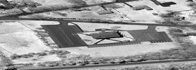
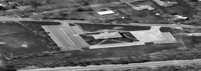
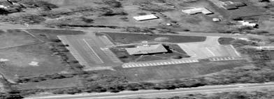
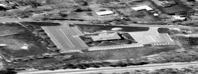
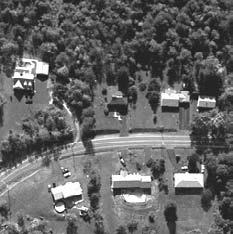
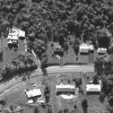
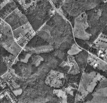
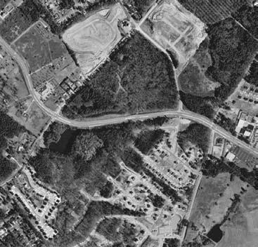
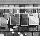
There are often trade-offs associated with the various resolutions that must be made when collecting remote sensing data (Figure 10;Color Plate 1).Generally, the higher the temp oral resolution requirement (e.g., monitoring hurricanes every half-hour), the lower the spatial resolution requirement (e.g., the NOAA GOES weather satellite records images with 4 × 4 to 8 × 8 km pixels). Conversely, the higher the spatial resolution requirement (e.g., monitoring urban land-use with 1 × 1 m data), the lower the temporal resolution requirement (e.g., every 1 to 10 years).For example,Figure 11 documents significant residential and commercial land-use development for an area near Atlanta, GA, using high spatial resolution (1 × 1 m) aerial photography obtained in 1993 and 1999. Some applications such as crop type or yield estimation might require relatively high temporal resolution data (e.g., multiple images obtained during a growing season) and moderate spatial resolution data (e.g., 250 ×250 m pixels). Emergency response applications may require very high spatial and temporal resolution data collection that generates tremendous amounts of data.
Another aspect of temporal information is how many observations are recorded from a single pulse of energy that is directed at the Earth by an active sensor such as LIDAR. For example, most LIDAR sensors emit one pulse of laser energy and record multiple responses from this pulse. Measuring the time differences between multiple responses allows for the determination of object heights and terrain structure. Also, the length of time required to emit an energy
signal by an active sensor is referred to as the pulse length Short pulse lengths allow precise distance (i.e., range) measurement.
Radiometric Information and Resolution
Some remote sensing systems record the reflected, emitted, or back-scattered electromagnetic radiation with more precision than other sensing systems. This is analogous to making a measurement with a ruler. If you want precisely to measure the length of an object, would you rather use a ruler with 16 or 1,024 subdivisions on it?
Radiometric resolution is defined as the sensitivity of a remote sensing detector to differences in signal strength as it records the radiant flux reflected, emitted, or back-scattered from the terrain. It defines the number of just discriminable signal levels. Therefore, radiometric resolution can have a significant impact on our ability to measure the properties of scene objects. The Landsat 1 Multispectral Scanner launched in 1972 recorded reflected energy with a precision of 6-bits (values ranging from 0 to 63). Landsat 4 and 5 Thematic Mapper sensors launched in 1982 and 1984, respectively, recorded data in 8 bits (values from 0 to 255) (Figure 12). Thus, the Landsat TM sensors had improved radiometric resolution (sensitivity) when compared with the original Landsat MSS. QuickBird and IKONOS sensors record information in 11 bits (values from 0 to 2,047). Several new sensor systems have 12-bit radiometric resolution (values ranging from 0 to 4,095). Radiometric resolution is sometimes referred to as the level of quantization. High radiometric resolution generally increases the probability that phenomena will be remotely sensed more accurately.
Polarization Information
The polarization characteristics of electromagnetic energy recorded by a remote sensing system are an important variable that can be used in many Earth resource investigations (Curran et al., 1998). Sunlight is polarized weakly. However, when sunlight strikes a nonmetal object (e.g., grass, forest, or concrete) it becomes depolarized and the incident energy is scattered differentially. Generally, the more smooth the surface, the greater the polarization. It is possible to use polarizing filters on passive remote sensing systems (e.g., aerial cameras) to record polarized light at various angles. It is also possible to selectively send and receive polarized energy using active remote sensing systems such as RADAR (e.g., horizontal send, vertical receive - HV; vertical send, horizontal receive - VH; vertical send, vertical receive - VV; horizontal send, horizontal receive - HH). Multiple-polarized
Remote Sensing of the Environment
Spatial and Temporal Resolution for Selected Applications
IncreasingSpatialandTemporalResolution
Crop Type, Yield
1 satellite: 16 day revisit
2 satellites: 8 day revisit
3 satellites: 4 day revisit Forestry Topography
Nominal Spatial Resolution
Figure 10 There are spatial and temporal resolution considerations that must be made for certain applications (Color Plate 1).
Digital Orthophotos of an Area near Atlanta, GA
Figure 11 Portions of digital-orthophoto-quarter-quads (DOQQ) of an area near Atlanta, GA. These data reside in the Georgia Spatial Data Infrastructure database and are useful for monitoring land-use change through time and the process of urbanization.
a. 1993 orthophoto. b. 1999 orthophoto.
Remote
Radiometric Resolution
7-bit (0 - 127)
8-bit (0 - 255) 9-bit (0 - 511)
(0 - 1023)
Figure 12 The radiometric resolution of a remote sensing system is the sensitivity of its detectors to differences in signal strength as they record the radiant flux reflected, emitted, or back-scattered from the terrain. The energy is normally quantized during an analogto-digital (A-to-D) conversion process to 8, 9, 10 bits or more.
RADAR imagery is an especially useful application of polarized energy.
Angular Information
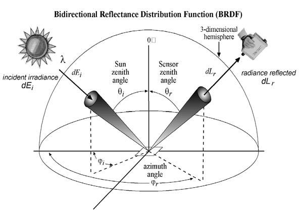
Remote sensing systems record very specific angular characteristics associated with each exposed silver halide crystal or pixel (Barnsley, 1999). The angular characteristics are a function of (Figure 13a):
• the location in a three-dimensional sphere of the illumination source (e.g., the Sun for a passive system or the sensor itself in the case of RADAR, LIDAR, and SONAR) and its associated azimuth and zenith angles,
• the orientation of the terrain facet (pixel) or terrain cover (e.g., vegetation) under investigation, and
• the location of the suborbital or orbital remote sensing system and its associated azimuth and zenith angles.
There is always an angle of incidence associated with the incoming energy that illuminates the terrain and an angle of exitance from the terrain to the sensor system. This bidirectional nature of remote sensing data collection is known to influence the spectral and polarization characteristics of the at-sensor radiance, L, recorded by the remote sensing system.
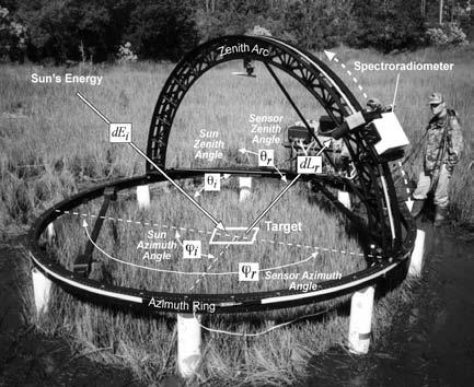
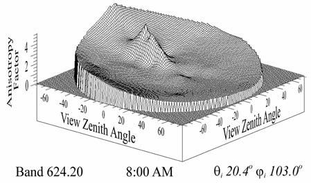
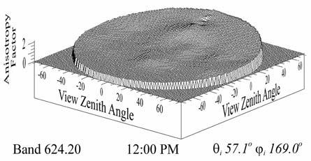
A goniometer can be used to document the changes in atsensor radiance, L, caused by changing the position of the sensor and/or the source of the illumination (e.g., the Sun) (Figure 13b). For example, Figure 13c presents three
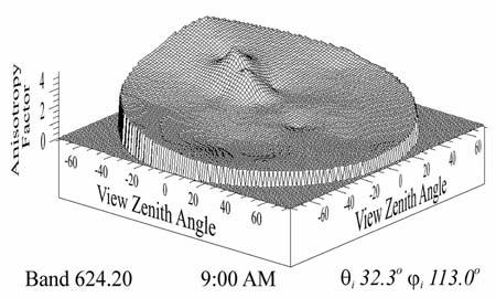
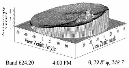
dimensional plots of smooth cordgrass (Spartina alterniflora) BRDF data collected at 8 a.m., 9 a.m., 12 p.m., and 4 p.m. on March 21, 2000, for band 624.20 nm. The only thing that changed between observations was the Sun’s azimuth and zenith angles. The azimuth and zenith angles of the spectroradiometer were held constant while viewing the smooth cordgrass. Ideally, the BRDF plots would be identical, suggesting that it does not matter what time of day we collect the remote sensor data because the spectral reflectance characteristics from the smooth cordgrass remain constant. It is clear that this is not the case and that the time of day influences the spectral response. The Multiangle Imaging Spectrometer (MISR) onboard the Terra satellite was designed to investigate the BRDF phenomena. Research continues on how to incorporate the BRDF information into the digital image processing system to improve our understanding of what is recorded in the remotely sensed imagery (Sandmeier, 2000; Schill et al., 2004).
Angular information is central to the use of remote sensor data in photogrammetric applications. Stereoscopic image analysis is based on the assumption that an object on the terrain is remotely sensed from two angles. Viewing the same terrain from two vantage points introduces stereoscopic parallax, which is the foundation for all stereoscopic photogrammetric and radargrammetric analysis (Light and Jensen, 2002).
Suborbital (Airborne) Remote Sensing Systems
High-quality photogrammetric cameras mounted onboard aircraft continue to provide aerial photography for many Earth resource applications. For example, the U.S. Geological Survey’s National Aerial Photography Program (NAPP) systematically collected l:40,000-scale black-and-white or color-infrared aerial photography of much of the United States every 5 to 10 years. Some of these photogrammetric data are now being collected using digital frame cameras. In addition, sophisticated remote sensing systems are routinely mounted on aircraft to provide high spatial and spectral resolution remotely sensed data. Examples include hyperspectral sensors such as NASA’s AVIRIS, the Canadian Airborne Imaging Spectrometer (CASI), and the Australian HyMap hyperspectral system. These sensors can collect data on demand when disaster strikes (e.g., oil spills or floods) if cloud-cover conditions permit. There are also numerous radars, such as Intermap’s Star-3i, that can be flown on aircraft day and night and in inclement weather. Unfortunately, suborbital remote sensor data are usually expensive to acquire per km2. Also, atmospheric turbulence can cause the data to have severe geometric distortions that can be difficult to correct.
Remote
Bidirectional Reflectance Distribution Function
a. Angular relationships.
b. Sandmeier Field Goniometer.
c. Comparison of hourly three-dimensional plots of BRDF for smooth cordgrass (Spartina alterniflora) data collected at 8 a.m., 9 a.m., 12 p.m., and 4 p.m. at the boardwalk site on March 21 – 22, 2000, for band 624.20 nm.
Figure 13 a) The concepts and parameters of the bidirectional reflectance distribution function (BRDF). A target is bathed in irradiance (dEi) from a specific Sun zenith and azimuth angle, and the sensor records the radiance (dLr) exiting the target of interest at a specific azimuth and zenith angle. b) The Sandmeier Field Goniometer collecting smooth cordgrass (Spartina alterniflora) BRDF measurements at North Inlet, SC. Spectral measurements are made at Sun zenith angle of θi and Sun azimuth angle of ϕi and a sensor zenith angle of view of θr and sensor azimuth angle of ϕr . A GER 3700 spectroradiometer, attached to the moving sled mounted on the zenith arc, records the amount of radiance leaving the target in 704 bands at 76 angles (Sandmeier, 2000; Schill et al., 2004). c) Hourly three-dimensional plots of BRDF data.
Remote Sensing of the Environment
Current and Proposed Satellite Remote Sensing Systems
Remote sensing systems onboard satellites provide highquality, relatively inexpensive data per km2. For example, the European Remote Sensing satellites (ERS-1 and 2) collect 26 × 28 m spatial resolution C-band active microwave (RADAR) imagery of much of Earth, even through clouds. Similarly, the Canadian Space Agency RADARSAT obtains C-band active microwave imagery. The United States has progressed from multispectral scanning systems (Landsat MSS launched in 1972) to more advanced scanning systems (Landsat 7 Enhanced Thematic Mapper Plus in 1999). The Land Remote Sensing Policy Act of 1992 specified the future of satellite land remote sensing programs in the United States (Asker, 1992; Jensen, 1992). Unfortunately, Landsat 6 with its Enhanced Thematic Mapper did not achieve orbit when launched on October 5, 1993. Landsat 7 was launched on April 15, 1999, to relieve the United States’ land remote sensing data gap. Unfortunately, it now has serious scan-line corrector problems. Meanwhile, the French have pioneered the development of linear array remote sensing technology with the launch of SPOT satellites 1 through 5 in 1986, 1990, 1993, 1998, and 2002.
The International Geosphere–Biosphere Program (IGBP) and the United States Global Change Research Program (USGCRP) call for scientific research to describe and understand the interactive physical, chemical, and biological processes that regulate the total Earth system. Space-based remote sensing is an integral part of these research programs because it provides the only means of observing global ecosystems consistently and synoptically. The National Aeronautics and Space Administration (NASA) Earth Science Enterprise (ESE) is the name given to the coordinated plan to provide the necessary satellite platforms and instruments and an Earth Observing System Data and Information System (EOSDIS), and related scientific research for IGBP. The Earth Observing System (EOS) is a series of Earth-orbiting satellites that will provide global observations for 15 years or more. The first satellites were launched in the late 1990s. EOS is complemented by missions and instruments from international partners. For example, the Tropical Rainfall Mapping Mission (TRMM) is a joint NASA/Japanese mission.
EOS Science Plan: Asrar and Dozier (1994) conceptualized the remote sensing science conducted as part of NASA’s ESE. They suggested that the Earth consists of two subsystems, 1) the physical climate, and 2) biogeochemical cycles, linked by the global hydrologic cycle, as shown in Figure 14.
The physical climate subsystem is sensitive to fluctuations in the Earth’s radiation balance. Human activities have caused changes to the planet’s radiative heating mechanism that rival or exceed natural change. Increases in greenhouse gases between 1765 and 1990 have caused a radiative forcing of 2.5 W m-2. If this rate is sustained, it could result in global mean temperatures increasing about 0.2 to 0.5 °C per decade during the next century. Volcanic eruptions and the ocean’s ability to absorb heat may impact the projections. Nevertheless, the following questions are being addressed using remote sensing (Asrar and Dozier, 1994):
•How do clouds, water vapor, and aerosols in the Earth’s radiation and heat budgets change with increased atmospheric greenhouse-gas concentrations?
•How do the oceans interact with the atmosphere in the transport and uptake of heat?
•How do land-surface properties such as snow and ice cover, evapotranspiration, urban/suburban land use, and vegetation influence circulation?
The Earth’s biogeochemical cycles have also been changed by humans. Atmospheric carbon dioxide has increased by 30 percent since 1859, methane by more than 100 percent, and ozone concentrations in the stratosphere have decreased, causing increased levels of ultraviolet radiation to reach the Earth’s surface. Global change research is addressing the following questions:
•What role do the oceanic and terrestrial components of the biosphere play in the changing global carbon budget?
•What are the effects on natural and managed ecosystems of increased carbon dioxide and acid deposition, shifting precipitation patterns, and changes in soil erosion, river chemistry, and atmospheric ozone concentrations?
The hydrologic cycle links the physical climate and biogeochemical cycles. The phase change of water between its gaseous, liquid, and solid states involves storage and release of latent heat, so it influences atmospheric circulation and globally redistributes both water and heat (Asrar and Dozier, 1994). The hydrologic cycle is the integrating process for the fluxes of water, energy, and chemical elements among components of the Earth system. Important questions to be addressed include these three:
•How will atmospheric variability, human activities, and climate change affect patterns of humidity, precipitation, evapotranspiration, and soil moisture?
Remote Sensing of the Environment
External
Cycles
Figure 14 The Earth system can be subdivided into two subsystems—the physical climate system and biogeochemical cycles—that are linked by the global hydrologic cycle. Significant changes in the external forcing functions and human activities have an impact on the physical climate system, biogeochemical cycles, and the global hydrologic cycle. Examination of these subsystems and their linkages defines the critical questions that the NASA Earth Observing System (EOS) is attempting to answer (adapted from Asrar and Dozier, 1994).
•How does soil moisture vary in time and space?
•Can we predict changes in the global hydrologic cycle using present and future observation systems and models?
These and other research questions are articulated in NASA’s current Earth System Science focus areas (Asrar, 2004). The models that address these research questions require sophisticated remote sensing measurements. To this end, the EOS Terra satellite was launched on December 18, 1999. It contains five remote sensing instruments (MODIS,
ASTER, MISR, CERES, and MOPITT) designed to address many of the research topics (King, 2003). The EOS Aqua satellite was launched in May, 2002. The Moderate Resolution Imaging Spectrometer (MODIS) has 36 bands from 0.405 to 14.385 μm that collect data at 250 ×250 m, 500 × 500 m, and 1 ×1 km spatial resolutions. MODIS views the entire surface of the Earth every one to two days, making observations in 36 spectral bands of land- and ocean-surface temperature, primary productivity, land-surface cover, clouds, aerosols, water vapor, temperature profiles, and fires.
The Advanced Spaceborne Thermal Emission and Reflection Radiometer (ASTER) has five bands in the thermal infrared region between 8 and 12 μm with 90-m pixels. It also has three broad bands between 0.5 and 0.9 μm with 15m pixels and stereo capability, and six bands in the shortwave infrared region (1.6 – 2.5 μm) with 30-m spatial resolution. ASTER is the highest spatial resolution sensor system on the EOS Terra platform and provides information on surface temperature that can be used to model evapotranspiration.
The Multiangle Imaging SpectroRadiometer (MISR) has nine separate charge-coupled-device (CCD) pushbroom cameras to observe the Earth in four spectral bands and at nine view angles. It provides data on clouds, atmospheric aerosols, and multiple-angle views of the Earth’s deserts, vegetation, and ice cover. The Clouds and the Earth’s Radiant Energy System (CERES) consists of two scanning radiometers that measure the Earth’s radiation balance and provide cloud property estimates to assess their role in radiative fluxes from the surface of the Earth to the top of the atmosphere. Finally, the Measurements of Pollution in the Troposphere (MOPITT) scanning radiometer provides information on the distribution, transport, sources, and sinks of carbon monoxide and methane in the troposphere.
The National Polar-orbiting Operational Environmental Satellite System (NPOESS) Preparatory Project (NPP) to be launched will extend key EOS measurements in support of long-term monitoring of climate trends and global biological productivity until the NPOESS can be launched sometime in the future. The NPP will contain MODIS-like instruments such as the Visible Infrared Imaging Radiometer Suite (VIIRS). With a five-year design life NPP will provide data past the designed lifetimes of EOS Terra and Aqua satellites through the launch of NPOESS (NOAA NPOESS, 2006).
Commercial Vendors: Space Imaging, Inc., launched IKONOS-2 on September 24, 1999. The IKONOS-2 sensor system has a 1 × 1 m panchromatic band and four 4 × 4 m
multispectral bands (Table 3). DigitalGlobe, Inc. , launched QuickBird on October 18, 2001, with a 61 × 61 cm panchromatic band and four 2.44 × 2.44 m multispectral bands. Orbimage, Inc. launched OrbView-3 on June 26, 2003, with 1 × 1 m panchromatic and 4 × 4 m multispectral bands.
Remote Sensing Data Analysis
Remote sensor data are analyzed using a variety of image processing techniques (Figures 5 and 15), including:
•analog (visual) image processing, and
•digital image processing.
Analog and digital analysis of remotely sensed data seek to detect and identify important phenomena in the scene. Once identified, the phenomena are usually measured, and the information is used in solving problems (Estes et al., 1983; Haack et al., 1997). Thus, both manual and digital analysis have the same general goals. However, the attainment of these goals may follow different paths.
Human beings are adept at visually interpreting images produced by certain types of remote sensing devices, especially cameras. One could ask, “Why try to mimic or improve on this capability?” First, there are certain thresholds beyond which the human interpreter cannot detect “just noticeable differences” in the imagery. For example, it is commonly known that an analyst can discriminate only about nine shades of gray when interpreting continuous-tone, blackand-white photography. If the data were originally recorded with 256 shades of gray, there might be more subtle information present in the image than the interpreter can extract visually. Furthermore, the interpreter brings to the task all the pressures of the day, making the interpretation subjective and generally unrepeatable. Conversely, the results obtained by computer are repeatable (even when wrong!). Also, when it comes to keeping track of a great amount of detailed quantitative information, such as the spectral characteristics of a vegetated field throughout a growing season for crop identification purposes, the computer is very adept at storing and manipulating such tedious information and possibly making a more definitive conclusion as to what crop is being grown. This is not to say that digital image processing is superior to visual image analysis. Rather, there may be times when a digital approach is better suited to the problem at hand. Optimum results are often achieved using a synergistic combination of both visual and digital image processing.
Figure 15 Analog (visual) and digital image processing of remotely sensed data use the elements of image interpretation.
Analog (Visual) Image Processing
Human beings use the fundamental elements of image interpretation summarized in Figure 15, including grayscale tone, color, height (depth), size, shape, shadow, texture, site, association, and arrangement. The human mind is amazingly good at recognizing and associating these complex elements in an image or photograph because we constantly process (a) profile views of Earth features every day and (b) images
seen in books, magazines, the television and the Internet. Furthermore, we are adept at bringing to bear all the knowledge in our personal background and collateral information. We then converge all this evidence to identify phenomena in images and judge their significance. Precise measurement of objects (length, area, perimeter, volume, etc.) may be performed using photogrammetric techniques applied to either monoscopic (single-photo) or stereoscopic (overlapping) images. Numerous books have been written on how to per-