Instant ebooks textbook Sears and zemansky's university physics with modern physics, technology upda
Sears
and Zemansky's University Physics with Modern Physics, Technology Update 13th International
Edition Hugh D. Young
Visit to download the full and correct content document: https://ebookmass.com/product/sears-and-zemanskys-university-physics-with-moder n-physics-technology-update-13th-international-edition-hugh-d-young/
More products digital (pdf, epub, mobi) instant download maybe you interests ...
All rights reserved. No part of this publication may be reproduced, stored in a retrieval system, or transmitted in any form or by any means, electronic, mechanical, photocopying, recording or otherwise, without either the prior written permission of the publisher or a licence permitting restricted copying in the United Kingdom issued by the Copyright Licensing Agency Ltd, Saffron House, 6–10 Kirby Street, London EC1N 8TS.
All trademarks used herein are the property of their respective owners. The use of any trademark in this text does not vest in the author or publisher any trademark ownership rights in such trademarks, nor does the use of such trademarks imply any affiliation with or endorsement of this book by such owners.
ISBN 10: 1-292-02063-6
ISBN 13: 978-1-292-02063-1
British Library Cataloguing-in-Publication Data
A catalogue record for this book is available from the British Library
7.
Hugh D. Young/Roger A. Freedman
Hugh D. Young/Roger A. Freedman
8. Momentum, Impulse, and Collisions
Hugh D. Young/Roger A. Freedman
Problem Set (Updated 13/e): Momentum, Impulse, and
Hugh D. Young/Roger A. Freedman
9. Rotation of Rigid Bodies
Hugh D. Young/Roger A. Freedman Problem
D. Young/Roger A. Freedman
Hugh D. Young/Roger A. Freedman
Hugh D. Young/Roger A. Freedman
Problem
12.
D. Young/Roger A.
Hugh D. Young/Roger A. Freedman Problem Set (Updated 13/e):
Hugh D. Young/Roger A. Freedman
14. Periodic Motion
Hugh D. Young/Roger A. Freedman Problem
Hugh D. Young/Roger A. Freedman
15.
Hugh D. Young/Roger A. Freedman Problem
Hugh D. Young/Roger A. Freedman
16. Sound and Hearing
Hugh D. Young/Roger A. Freedman
Problem Set (Updated 13/e): Sound and Hearing
Hugh D. Young/Roger A. Freedman
17. Temperature and Heat
Hugh D. Young/Roger A. Freedman
Problem Set (Updated 13/e): Temperature and Heat
Hugh D. Young/Roger A. Freedman
18. Thermal Properties of Matter
Hugh D. Young/Roger A. Freedman
Problem Set (Updated 13/e): Thermal Properties of Matter
Hugh D. Young/Roger A. Freedman
19. The First Law of Thermodynamics
Hugh D. Young/Roger A. Freedman
Problem Set (Updated 13/e): The First Law of Thermodynamics
Hugh D. Young/Roger A. Freedman
20. The Second Law of Thermodynamics
Hugh D. Young/Roger A. Freedman
Problem Set (Updated 13/e): The Second Law of Thermodynamics
Hugh D. Young/Roger A. Freedman
21. Electric Charge and Electric Field
Hugh D. Young/Roger A. Freedman
Problem
(Updated 13/e):
Hugh D. Young/Roger A. Freedman
22. Gauss's Law
Hugh D. Young/Roger A. Freedman
Problem Set (Updated 13/e): Gauss's Law
Hugh D. Young/Roger A. Freedman
23. Electric Potential
Hugh D. Young/Roger A. Freedman
Problem Set (Updated 13/e): Electric Potential
Hugh D. Young/Roger A. Freedman
24. Capacitance and Dielectrics
Hugh D. Young/Roger A. Freedman
Problem Set (Updated 13/e): Capacitance and Dielectrics
Hugh D. Young/Roger A. Freedman
25. Current, Resistance, and Electromotive Force
Hugh D. Young/Roger A. Freedman
Problem Set (Updated 13/e): Current, Resistance, and Electromotive Force
Hugh D. Young/Roger A. Freedman
26. Direct-Current Circuits
Hugh D. Young/Roger A. Freedman
Problem Set (Updated 13/e): Direct-Current Circuits
Hugh D. Young/Roger A. Freedman
27. Magnetic Field and Magnetic Forces
Hugh D. Young/Roger A. Freedman
Problem Set (Updated 13/e): Magnetic Field and Magnetic Forces
Hugh D. Young/Roger A. Freedman
28. Sources of Magnetic Field
Hugh D. Young/Roger A. Freedman
Problem Set (Updated 13/e): Sources of Magnetic Field
Hugh D. Young/Roger A. Freedman
29. Electromagnetic Induction
Hugh D. Young/Roger A. Freedman
Problem Set (Updated 13/e): Electromagnetic Induction
Hugh D. Young/Roger A. Freedman
30.
Hugh D. Young/Roger A. Freedman
Problem
(Updated 13/e): Inductance
Hugh D. Young/Roger A. Freedman
31. Alternating Current
Hugh D. Young/Roger A. Freedman
Problem Set (Updated 13/e): Alternating Current
Hugh D. Young/Roger A. Freedman
32. Electromagnetic Waves
Hugh D. Young/Roger A. Freedman
Problem Set (Updated 13/e): Electromagnetic Waves
Hugh D. Young/Roger A. Freedman
33. The Nature and Propagation of Light
Hugh D. Young/Roger A. Freedman
Problem Set (Updated 13/e): The Nature and Propagation of Light
Hugh D. Young/Roger A. Freedman
34. Geometric Optics
Hugh D. Young/Roger A. Freedman
Problem Set (Updated 13/e): Geometric Optics
Hugh D. Young/Roger A. Freedman
35. Interference
Hugh D. Young/Roger A. Freedman
Problem Set (Updated 13/e): Interference
Hugh D. Young/Roger A. Freedman
36. Diffraction
Hugh D. Young/Roger A. Freedman
Problem Set (Updated 13/e): Diffraction
Hugh D. Young/Roger A. Freedman
37. Relativity
Hugh D. Young/Roger A. Freedman
Problem Set (Updated 13/e): Relativity
Hugh D. Young/Roger A. Freedman
38. Photons: Light Waves Behaving as Particles
Hugh D. Young/Roger A. Freedman
Problem Set (Updated 13/e): Photons: Light Waves Behaving as Particles
Hugh D. Young/Roger A. Freedman
39. Particles Behaving as Waves
Hugh D. Young/Roger A. Freedman
Problem Set (Updated 13/e): Particles
Hugh D. Young/Roger A. Freedman
40. Quantum Mechanics
Hugh D. Young/Roger A. Freedman
Problem Set (Updated 13/e): Quantum Mechanics
Hugh D. Young/Roger A. Freedman
41. Atomic Structure
Hugh D. Young/Roger A. Freedman
Problem Set (Updated 13/e): Atomic Structure
Hugh D. Young/Roger A. Freedman
42. Molecules and Condensed Matter
Hugh D. Young/Roger A. Freedman
Problem Set (Updated 13/e): Molecules and Condensed Matter
Hugh D. Young/Roger A. Freedman
43. Nuclear Physics
Hugh D. Young/Roger A. Freedman
Problem Set (Updated 13/e): Nuclear Physics
Hugh D. Young/Roger A. Freedman
44. Particle Physics and Cosmology
Hugh D. Young/Roger A. Freedman
Problem Set (Updated 13/e): Particle Physics and Cosmology
Hugh D. Young/Roger A. Freedman
Appendix: The International System of Units
Hugh D. Young/Roger A. Freedman
Appendix: The Greek Alphabet
Hugh D. Young/Roger A. Freedman
Appendix: Periodic Table of the Elements
Hugh D. Young/Roger A. Freedman
HOW TO SUCCEED IN PHYSICS BY REALLY TRYING
MarkHollabaugh NormandaleCommunityCollege
Physics encompasses the large and the small, the old and the new. From the atom to galaxies, from electrical circuitry to aerodynamics, physics is very much a part of the world around us. You probably are taking this introductory course in calculusbased physics because it is required for subsequent courses you plan to take in preparation for a career in science or engineering. Your professor wants you to learn physics and to enjoy the experience. He or she is very interested in helping you learn this fascinating subject. That is part of the reason your professor chose this textbook for your course. That is also the reason Drs. Young and Freedman asked me to write this introductory section. We want you to succeed!
The purpose of this section of University Physics is to give you some ideas that will assist your learning. Specific suggestions on how to use the textbook will follow a brief discussion of general study habits and strategies.
Preparation for This Course
If you had high school physics, you will probably learn concepts faster than those who have not because you will be familiar with the language of physics. If English is a second language for you, keep a glossary of new terms that you encounter and make sure you understand how they are used in physics. Likewise, if you are farther along in your mathematics courses, you will pick up the mathematical aspects of physics faster. Even if your mathematics is adequate, you may find a book such as Arnold D. Pickar’s Preparing for General Physics: Math Skill Drills and Other Useful Help (Calculus Version) to be useful. Your professor may actually assign sections of this math review to assist your learning.
Learning to Learn
Each of us has a different learning style and a preferred means of learning. Understanding your own learning style will help you to focus on aspects of physics that may give you difficulty and to use those components of your course that will help you overcome the difficulty. Obviously you will want to spend more time on those aspects that give you the most trouble. If you learn by hearing, lectures will be very important. If you learn by explaining, then working with other students will be useful to you. If solving problems is difficult for you, spend more time learning how to solve problems. Also, it is important to understand and develop good study habits. Perhaps the most important thing you can do for yourself is to set aside adequate, regularly scheduled study time in a distraction-free environment.
Answer the following questions for yourself:
•Am I able to use fundamental mathematical concepts from algebra, geometry and trigonometry? (If not, plan a program of review with help from your professor.)
•In similar courses, what activity has given me the most trouble? (Spend more time on this.) What has been the easiest for me? (Do this first; it will help to build your confidence.)
From the Preface of University Physics with Modern Physics, Technology Update, 13th Edition. Hugh D. Young, Roger A. Freedman.
•Do I understand the material better if I read the book before or after the lecture? (You may learn best by skimming the material, going to lecture, and then undertaking an in-depth reading.)
•Do I spend adequate time in studying physics? (A rule of thumb for a class like this is to devote, on the average, 2.5 hours out of class for each hour in class. For a course meeting 5 hours each week, that means you should spend about 10 to 15 hours per week studying physics.)
•Do I study physics every day? (Spread that 10 to 15 hours out over an entire week!) At what time of the day am I at my best for studying physics? (Pick a specific time of the day and stick to it.)
•Do I work in a quiet place where I can maintain my focus? (Distractions will break your routine and cause you to miss important points.)
Working with Others
Scientists or engineers seldom work in isolation from one another but rather workcooperatively. You will learn more physics and have more fun doing it if youwork with other students. Some professors may formalize the use of cooperativelearning or facilitate the formation of study groups. You may wish to form your own informal study group with members of your class who live in your neighborhood or dorm. If you have access to e-mail, use it to keep in touch with one another. Your study group is an excellent resource when reviewing for exams.
Lectures and Taking Notes
An important component of any college course is the lecture. In physics this is especially important because your professor will frequently do demonstrations of physical principles, run computer simulations, or show video clips. All of these are learning activities that will help you to understand the basic principles of physics. Don’t miss lectures, and if for some reason you do, ask a friend or member of your study group to provide you with notes and let you know what happened.
Take your class notes in outline form, and fill in the details later. It can be very difficult to take word for word notes, so just write down key ideas. Your professor may use a diagram from the textbook. Leave a space in your notes and just add the diagram later. After class, edit your notes, filling in any gaps or omissions and noting things you need to study further. Make references to the textbook by page, equation number, or section number.
Make sure you ask questions in class, or see your professor during office hours. Remember the only “dumb” question is the one that is not asked. Your college may also have teaching assistants or peer tutors who are available to help you with difficulties you may have.
Examinations
Taking an examination is stressful. But if you feel adequately prepared and are well-rested, your stress will be lessened. Preparing for an exam is a continual process; it begins the moment the last exam is over. You should immediately go over the exam and understand any mistakes you made. If you worked a problem and made substantial errors, try this: Take a piece of paper and divide it down the middle with a line from top to bottom. In one column, write the proper solution to the problem. In the other column, write what you did and why, if you know, and why your solution was incorrect. If you are uncertain why you made your mistake, or how to avoid making it again, talk with your professor. Physics continually builds on fundamental ideas and it is important to correct any misunderstandings immediately. Warning: While cramming at the last minute may get you through the presentexam, you will not adequately retain the concepts for use on the nextexam.
TO THE INSTRUCTOR
PREFACE
This book is the product of more than six decades of leadership and innovation in physics education. When the first edition of University Physics by Francis W. Sears and Mark W. Zemansky was published in 1949, it was revolutionary amongcalculus-based physics textbooks in its emphasis on the fundamental principles of physics and how to apply them. The success of University Physics with generations of several million students and educators around the world is a testament to the merits of this approach, and to the many innovations it has introduced subsequently.
In preparing this new Thirteenth Edition, we have further enhanced and developed University Physics to assimilate the best ideas from education research with enhanced problem-solving instruction, pioneering visual and conceptual pedagogy, the first systematically enhanced problems, and the most pedagogically proven and widely used online homework and tutorial system in the world.
New to This Edition
•Included in each chapter, Bridging Problems provide a transition between the single-concept Examples and the more challenging end-of-chapter problems. Each Bridging Problem poses a difficult, multiconcept problem, which often incorporates physics from earlier chapters. In place of a full solution, it provides a skeleton Solution Guide consisting of questions and hints, which helps train students to approach and solve challenging problems with confidence.
• All Examples, Conceptual Examples, and Problem-Solving Strategies are revised to enhance conciseness and clarity for today’s students.
•The core modern physics chapters (Chapters 38–41) are revised extensively to provide a more idea-centered, less historical approach to the material. Chapters 42–44are also revised significantly.
• The fluid mechanics chapternow precedes the chapters on gravitation and periodic motion, so that the latter immediately precedes the chapter on mechanical waves.
• Additional bioscience applications appear throughout the text, mostly in the form of marginal photos with explanatory captions, to help students see how physics is connected to many breakthroughs and discoveries in the biosciences.
•The text has been streamlined for tighter and more focused language.
• Using data from MasteringPhysics, changes to the end-of-chaptercontent include the following:
• 15%–20% of problems are new.
• The number and level of calculus-requiring problems has been increased.
•Most chapters include five to seven biosciences-related problems.
•The number of cumulative problems (those incorporating physics from earlier chapters) has been increased.
• Over70 PhETsimulations are linked to the Pearson eText and provided in the Study Area of the MasteringPhysics website (with icons in the print text). These powerful simulations allow students to interact productively with the physics concepts they are learning. PhETclicker questions are also included on the Instructor Resource DVD.
• Video Tutors bring key content to life throughout the text:
• Dozens of Video Tutors feature “pause-and-predict” demonstrations of key physics concepts and incorporate assessment as the student progresses to actively engage the student in understanding the key conceptual ideas underlying the physics principles.
Standard,Extended, and Three-Volume Editions
With MasteringPhysics:
• Standard Edition: Chapters 1–37 (ISBN 978-0-321-69688-5)
• Every Worked Example in the book is accompanied by a Video Tutor Solution that walks students through the problem-solving process, providing a virtual teaching assistant on a round-the-clock basis.
• All of these Video Tutors play directly through links within the Pearson eText. Many also appear in the Study Area within MasteringPhysics.
Key Features of University Physics
•Deep and extensive problem sets cover a wide range of difficulty and exerciseboth physical understanding and problem-solving expertise. Many problems are based on complex real-life situations.
•This text offers a larger number of Examples and Conceptual Examples than any other leading calculus-based text, allowing it to explore problem-solving challenges not addressed in other texts.
•A research-based problem-solving approach (Identify, Set Up, Execute, Evaluate) is used not just in every Example but also in the Problem-Solving Strategies and throughout the Student and Instructor Solutions Manuals and the Study Guide. This consistent approach teaches students to tackle problems thoughtfully rather than cutting straight to the math.
• Problem-Solving Strategies coach students in how to approach specific types of problems.
•The Figures use a simplified graphical style to focus on the physics of a situation, and they incorporate explanatory annotation. Both techniques have been demonstrated to have a strong positive effect on learning.
•Figures that illustrate Example solutions often take the form of black-andwhite pencil sketches, which directly represent what a student should draw in solving such a problem.
•The popular Caution paragraphs focus on typical misconceptions and student problem areas.
•End-of-section Test Your Understanding questions let students check their grasp of the material and use a multiple-choice or ranking-task format to probe for common misconceptions.
• Visual Summaries at the end of each chapter present the key ideas in words, equations, and thumbnail pictures, helping students to review more effectively.
Instructor Supplements
Note: For convenience, all of the following instructor supplements (except for the Instructor Resource DVD) can be downloaded from the Instructor Area, accessed via the left-hand navigation bar of MasteringPhysics (www.masteringphysics.com).
Instructor Solutions, prepared by A. Lewis Ford (Texas A&M University) and Wayne Anderson, contain complete and detailed solutions to all end-ofchapter problems. All solutions follow consistently the same Identify/Set Up/ Execute/Evaluate problem-solving framework used in the textbook. Download only from the MasteringPhysics Instructor Area or from the Instructor Resource Center (www.pearsonhighered.com/irc).
The cross-platform Instructor Resource DVD (ISBN 978-0-321-69661-8) provides a comprehensive library of more than 420 applets from ActivPhysics OnLine as well as all line figures from the textbook in JPEG format. In addition, all the key equations, problem-solving strategies, tables, and chapter summaries are provided in editable Word format. In-class weekly multiple-choice questions for use with various Classroom Response Systems (CRS) are also provided, based on the Test Your Understanding questions in the text. Lecture outlines in PowerPoint are also included along with over 70 PhET simulations.
MasteringPhysics® (www.masteringphysics.com) is the most advanced, educationally effective, and widely used physics homework and tutorial system in the world. Eight years in development, it provides instructors with a library of extensively pre-tested end-of-chapter problems and rich, multipart, multistep tutorials that incorporate a wide variety of answer types, wrong answer feedback, individualized help (comprising hints or simpler sub-problems upon request), all driven by the largest metadatabase of student problem-solving in the world. NSFsponsored published research (and subsequent studies) show that MasteringPhysics has dramatic educational results. MasteringPhysics allows instructors to build wide-ranging homework assignments of just the right difficulty and length and provides them with efficient tools to analyze both class trends, and the work of any student in unprecedented detail.
MasteringPhysics routinely provides instant and individualized feedback and guidance to more than 100,000 students every day. A wide range of tools and support make MasteringPhysics fast and easy for instructors and students to learn to use. Extensive class tests show that by the end of their course, an unprecedented eight of nine students recommend MasteringPhysics as their preferred way to study physics and do homework.
MasteringPhysics enables instructors to:
•Quickly build homework assignments that combine regular end-of-chapter problems and tutoring (through additional multi-step tutorial problems that offer wrong-answer feedback and simpler problems upon request).
•Expand homework to include the widest range of automatically graded activities available—from numerical problems with randomized values, through algebraic answers, to free-hand drawing.
•Choose from a wide range of nationally pre-tested problems that provide accurate estimates of time to complete and difficulty.
•After an assignment is completed, quickly identify not only the problems that were the trickiest for students but the individual problem types where students had trouble.
•Compare class results against the system’s worldwide average for each problem assigned, to identify issues to be addressed with just-in-time teaching.
•Check the work of an individual student in detail, including time spent on eachproblem, what wrong answers they submitted at each step, how much help they asked for, and how many practice problems they worked.
ActivPhysicsOnLine™ (which is accessed through the Study Area within www.masteringphysics.com) provides a comprehensive library of more than 420 tried and tested ActivPhysics applets updated for web delivery using the latest online technologies. In addition, it provides a suite of highly regarded appletbased tutorials developed by education pioneers Alan Van Heuvelen and Paul D’Alessandris. Margin icons throughout the text direct students to specific exercises that complement the textbook discussion.
The online exercises are designed to encourage students to confront misconceptions, reason qualitatively about physical processes, experiment quantitatively, and learn to think critically. The highly acclaimed ActivPhysics OnLine companion workbooks help students work through complex concepts and understand them more clearly. More than 420 applets from the ActivPhysics OnLine library are also available on the Instructor Resource DVD for this text.
The Test Bank contains more than 2,000 high-quality problems, with a range of multiple-choice, truefalse, short-answer, and regular homework-type questions. Test files are provided both in TestGen (an easy-to-use, fully networkable program for creating and editing quizzes and exams) and Word format. Download only from the MasteringPhysics Instructor Area or from the Instructor Resource Center (www.pearsonhighered.comirc). > >
Five Easy Lessons: Strategies for Successful Physics Teaching (ISBN 978-0805-38702-5) by Randall D. Knight (California Polytechnic State University, San Luis Obispo) is packed with creative ideas on how to enhance any physics course. It is an invaluable companion for both novice and veteran physics instructors.
Student Supplements
The Study Guide by Laird Kramer reinforces the text’s emphasis on problemsolving strategies and student misconceptions. The Study Guide for Volume 1 (ISBN 978-0-321-69665-6) covers Chapters 1–20, and the Study Guide for Volumes 2 and 3 (ISBN 978-0-321-69669-4) covers Chapters 21–44.
The Student Solutions Manual by Lewis Ford (Texas A&M University) and Wayne Anderson contains detailed, step-by-step solutions to more than half of the odd-numbered end-of-chapter problems from the textbook. All solutions follow consistently the same Identify/Set Up/Execute/Evaluate problem-solving framework used in the textbook. The Student Solutions Manual for Volume 1 (ISBN 978-0-321-69668-7)covers Chapters 1–20, and the Student Solutions Manual for Volumes 2 and 3 (ISBN 978-0-321-69667-0) covers Chapters 21–44.
MasteringPhysics® (www.masteringphysics.com) is a homework, tutorial, and assessment system based on years of research into how students work physics problems and precisely where they need help. Studies show that students who use MasteringPhysics significantly increase their scores compared to hand-written homework. MasteringPhysics achieves this improvement by providing students with instantaneous feedback specific to their wrong answers, simpler sub-problems upon request when they get stuck, and partial credit for their method(s). This individualized, 247 Socratic tutoring is recommended by nine out of ten students to their peers as the most effective and time-efficient way to study.
Pearson eText is available through MasteringPhysics, either automatically when MasteringPhysics is packaged with new books, or available as a purchased upgrade online. Allowing students access to the text wherever they have access to the Internet, Pearson eText comprises the full text, including figures that can be enlarged for better viewing. With eText, students are also able to pop up definitions and terms to help with vocabulary and the reading of the material. Students can also take notes in eText using the annotation feature at the top of each page.
Pearson Tutor Services (www.pearsontutorservices.com). Each student’s subscriptionto MasteringPhysics also contains complimentary access to Pearson Tutor Services, powered by Smarthinking, Inc. By logging in with their MasteringPhysicsID and password, students will be connected to highly qualified e-instructors who provide additional interactive online tutoring on the major concepts of physics. Some restrictions apply; offer subject to change.
ActivPhysicsOnLine™ (which is accessed through the Study Area within www.masteringphysics.com) provides students with a suite of highly regarded applet-based tutorials (see above). The following workbooks help students work through complex concepts and understand them more clearly.
We would like to thank the hundreds of reviewers and colleagues who have offered valuable comments and suggestions over the life of this textbook. The continuing success of University Physics is due in large measure to their contributions.
Edward Adelson (Ohio State University), Ralph Alexander (University of Missouri at Rolla), J. G. Anderson, R. S. Anderson, Wayne Anderson (Sacramento City College), Alex Azima (Lansing Community College), Dilip Balamore (Nassau Community College), Harold Bale (University of North Dakota), Arun Bansil (Northeastern University), John Barach (Vanderbilt University), J. D. Barnett, H. H. Barschall, Albert Bartlett (University of Colorado), Marshall Bartlett (Hollins University), Paul Baum (CUNY, Queens College), Frederick Becchetti (University of Michigan), B. Bederson, David Bennum (University of Nevada, Reno), Lev I. Berger (San Diego State University), Robert Boeke (William Rainey Harper College), S. Borowitz, A. C. Braden, James Brooks (Boston University), Nicholas E. Brown (California Polytechnic State University, San Luis Obispo), Tony Buffa (California Polytechnic State University, San Luis Obispo), A. Capecelatro, Michael Cardamone (Pennsylvania State University), Duane Carmony (Purdue University), Troy Carter (UCLA), P. Catranides, John Cerne (SUNY at Buffalo), Tim Chupp (University of Michigan), Shinil Cho (La Roche College), Roger Clapp (University of South Florida), William M. Cloud (Eastern Illinois University), Leonard Cohen (Drexel University), W. R. Coker (University of Texas, Austin), Malcolm D. Cole (University of Missouri at Rolla), H. Conrad, David Cook (Lawrence University), Gayl Cook (University of Colorado), Hans Courant (University of Minnesota), Bruce A. Craver (University of Dayton), Larry Curtis (University of Toledo), Jai Dahiya (Southeast Missouri State University), Steve Detweiler (University of Florida), George Dixon (Oklahoma State University), Donald S. Duncan, Boyd Edwards (West Virginia University), Robert Eisenstein (Carnegie Mellon University), Amy Emerson Missourn (Virginia Institute of Technology), William Faissler (Northeastern University), William Fasnacht (U.S. Naval Academy), Paul Feldker (St. Louis Community College), Carlos Figueroa (Cabrillo College), L. H. Fisher, Neil Fletcher (Florida State University), Robert Folk, Peter Fong (Emory University), A. Lewis Ford (Texas A&M University), D. Frantszog, James R. Gaines (Ohio State University), Solomon Gartenhaus (Purdue University), Ron Gautreau (New Jersey Institute of Technology), J. David Gavenda (University of Texas, Austin), Dennis Gay (University of North Florida), James Gerhart (University of Washington), N. S. Gingrich, J. L. Glathart, S. Goodwin, Rich Gottfried (Frederick Community College), Walter S. Gray (University of Michigan), Paul Gresser (University of Maryland), Benjamin Grinstein (UC San Diego), Howard Grotch (Pennsylvania State University), John Gruber (San Jose State University), Graham D. Gutsche (U.S. Naval Academy), Michael J. Harrison (Michigan State University), Harold Hart (Western Illinois University), Howard Hayden (University of Connecticut), Carl Helrich (Goshen College), Laurent Hodges (Iowa State University), C. D. Hodgman, Michael Hones (Villanova University), Keith Honey (West Virginia Institute of Technology), Gregory Hood (Tidewater Community College), John Hubisz (North Carolina State University), M. Iona, John Jaszczak (Michigan Technical University), Alvin Jenkins (North Carolina State University), Robert P. Johnson (UC Santa Cruz), Lorella Jones (University of Illinois), John Karchek (GMI Engineering & Management Institute), Thomas Keil (Worcester Polytechnic Institute), Robert Kraemer (Carnegie Mellon University), Jean P. Krisch (University of Michigan), Robert A. Kromhout, Andrew Kunz (Marquette University), Charles Lane (Berry College), Thomas N. Lawrence (Texas State University), Robert J. Lee, Alfred Leitner (Rensselaer Polytechnic University), Gerald P. Lietz (De Paul University), Gordon Lind (Utah State University), S. Livingston, Elihu Lubkin (University of Wisconsin, Milwaukee), Robert Luke (Boise State University), David Lynch (Iowa State University), Michael Lysak (San Bernardino Valley College), Jeffrey Mallow (Loyola University), Robert Mania (Kentucky State University), Robert Marchina (University of Memphis), David Markowitz (University of Connecticut), R. J. Maurer, Oren Maxwell (Florida International University), Joseph L. McCauley (University of Houston), T. K. McCubbin, Jr. (Pennsylvania State University), Charles McFarland (University of Missouri at Rolla), James Mcguire (Tulane University), Lawrence McIntyre (University of Arizona), Fredric Messing (Carnegie-Mellon University), Thomas Meyer (Texas A&M University), Andre Mirabelli (St. Peter’s College, New Jersey), Herbert Muether (S.U.N.Y., Stony Brook), Jack Munsee (California State University, Long Beach), Lorenzo Narducci (Drexel University), Van E. Neie (Purdue University), David A. Nordling (U. S. Naval Academy), Benedict Oh (Pennsylvania State University), L. O. Olsen, Jim Pannell (DeVry Institute of Technology), W. F. Parks (University of Missouri), Robert Paulson (California State University, Chico), Jerry Peacher (University of Missouri at Rolla), Arnold Perlmutter (University of Miami), Lennart Peterson (University of Florida), R. J. Peterson (University of Colorado, Boulder), R. Pinkston, Ronald Poling (University of Minnesota), J. G. Potter, C. W. Price (Millersville University), Francis Prosser (University of Kansas), Shelden H. Radin, Roberto Ramos (Drexel University), Michael Rapport (Anne Arundel Community College), R. Resnick, James A. Richards, Jr., John S. Risley (North Carolina State University), Francesc Roig (University of California, Santa Barbara), T. L. Rokoske, Richard Roth (Eastern Michigan University), Carl Rotter (University of West Virginia), S. Clark Rowland (Andrews University), Rajarshi Roy (Georgia Institute of Technology), Russell A. Roy (Santa Fe Community College), Dhiraj Sardar (University of Texas, San Antonio), Bruce Schumm (UC Santa Cruz), Melvin Schwartz (St. John’s University), F. A. Scott, L. W. Seagondollar, Paul Shand (University of Northern Iowa), Stan Shepherd (Pennsylvania State University), Douglas Sherman (San Jose State), Bruce Sherwood (Carnegie Mellon University), Hugh Siefkin (Greenville College), Tomasz Skwarnicki (Syracuse University), C. P. Slichter, Charles W. Smith (University of Maine, Orono), Malcolm Smith (University of Lowell), Ross Spencer (Brigham Young University), Julien Sprott (University of Wisconsin), Victor Stanionis (Iona College), James Stith (American Institute of Physics), Chuck Stone (North Carolina A&T State
University), Edward Strother (Florida Institute of Technology), Conley Stutz (Bradley University), Albert Stwertka (U.S. Merchant Marine Academy), Kenneth Szpara-DeNisco (Harrisburg Area Community College), Martin Tiersten (CUNY, City College), David Toot (Alfred University), Somdev Tyagi (Drexel University), F. Verbrugge, Helmut Vogel (Carnegie Mellon University), Robert Webb (Texas A & M), Thomas Weber (Iowa State University), M. Russell Wehr, (Pennsylvania State University), Robert Weidman (Michigan Technical University), Dan Whalen (UC San Diego), Lester V. Whitney, Thomas Wiggins (Pennsylvania State University), David Willey (University of Pittsburgh, Johnstown), George Williams (University of Utah), John Williams (Auburn University), Stanley Williams (Iowa State University), Jack Willis, Suzanne Willis (Northern Illinois University), Robert Wilson (San Bernardino Valley College), L. Wolfenstein, James Wood (Palm Beach Junior College), Lowell Wood (University of Houston), R. E. Worley, D. H. Ziebell (Manatee Community College), George O. Zimmerman (Boston University)
In addition, we both have individual acknowledgments we would like to make. I want to extend my heartfelt thanks to my colleagues at Carnegie Mellon, especially Professors Robert Kraemer, Bruce Sherwood, Ruth Chabay, Helmut Vogel, and Brian Quinn, for many stimulating discussions about physics pedagogy and for their support and encouragement during the writing of several successive editions of this book. I am equally indebted to the many generations of Carnegie Mellon students who have helped me learn what good teaching and good writing are, by showing me what works and what doesn’t. It is always a joy and a privilege to express my gratitude to my wife Alice and our children Gretchen and Rebecca for their love, support, and emotional sustenance during the writing of several successive editions of this book. May all men and women be blessed with love such as theirs. — H. D. Y.
I would like to thank my past and present colleagues at UCSB, including Rob Geller, Carl Gwinn, Al Nash, Elisabeth Nicol, and Francesc Roig, for their wholehearted support and for many helpful discussions. I owe a special debt of gratitude to my early teachers Willa Ramsay, Peter Zimmerman, William Little, Alan Schwettman, and Dirk Walecka for showing me what clear and engaging physics teaching is all about, and to Stuart Johnson for inviting me to become a co-author of University Physics beginning with the 9th edition. I want to express special thanks to the editorial staff at Addison-Wesley and their partners: to Nancy Whilton for her editorial vision; to Margot Otway for her superb graphic sense and careful development of this edition; to Peter Murphy for his contributions to the worked examples; to Jason J. B. Harlow for his careful reading of the page proofs; and to Chandrika Madhavan, Steven Le, and Cindy Johnson for keeping the editorial and production pipeline flowing. Most of all, I want to express my gratitude and love to my wife Caroline, to whom I dedicate my contribution to this book. Hey, Caroline, the new edition’s done at last — let’s go flying! — R. A. F.
Please Tell Us What You Think!
We welcome communications from students and professors, especially concerning errors or deficiencies that you find in this edition. We have devoted a lot of time and effort to writing the best book we know how to write, and we hope it will help you to teach and learn physics. In turn, you can help us by letting us know what still needs to be improved! Please feel free to contact us either electronically or by ordinary mail. Your comments will be greatly appreciated.
December 2010
Hugh D. YoungRoger A. Freedman Department of PhysicsDepartment of Physics Carnegie Mellon UniversityUniversity of California, Santa Barbara Pittsburgh, PA 15213Santa Barbara, CA 93106-9530 hdy@andrew.cmu.eduairboy@physics.ucsb.edu http://www.physics.ucsb.edu/~airboy/
UNITS, PHYSICAL QUANTITIES, AND VECTORS
?Being able to predict the path of a thunderstorm is essential for minimizing thedamage it does to lives and property. If a thunderstorm is moving at 20kmh in a direction 53°north of east, how far north does the thunderstorm move in 1 h?
Physics is one of the most fundamental of the sciences. Scientists of all disciplines use the ideas of physics, including chemists who study the structure of molecules, paleontologists who try to reconstruct how dinosaurs walked, and climatologists who study how human activities affect the atmosphere and oceans. Physics is also the foundation of all engineering and technology. No engineer could design a flat-screen TV, an interplanetary spacecraft, or even a better mousetrap without first understanding the basic laws of physics.
The study of physics is also an adventure. You will find it challenging, sometimes frustrating, occasionally painful, and often richly rewarding. If you’ve ever wondered why the sky is blue, how radio waves can travel through empty space, or how a satellite stays in orbit, you can find the answers by using fundamental physics. You will come to see physics as a towering achievement of the human intellect in its quest to understand our world and ourselves.
In this chapter, we’ll go over some important preliminaries that we’ll need throughout our study. We’ll discuss the nature of physical theory and the use of idealized models to represent physical systems. We’ll introduce the systems of units used to describe physical quantities and discuss ways to describe the accuracy of a number. We’ll look at examples of problems for which we can’t (or don’t want to) find a precise answer, but for which rough estimates can be useful and interesting. Finally, we’ll study several aspects of vectors and vector algebra. Vectors will be needed throughout our study of physics to describe and analyze physical quantities, such as velocity and force, that have direction as well as magnitude.
LEARNING GOALS
By studying this chapter, you will learn:
•Three fundamental quantities of physics and the units physicists use to measure them.
•How to keep track of significant figures in your calculations.
•The difference between scalars and vectors, and how to add and subtract vectors graphically.
•What the components of a vector are, and how to use them in calculations.
•What unit vectors are, and how to use them with components to describe vectors.
•Two ways of multiplying vectors.
Hugh D. Young, Roger A. Freedman.
Ralph Wetmore/Getty Images
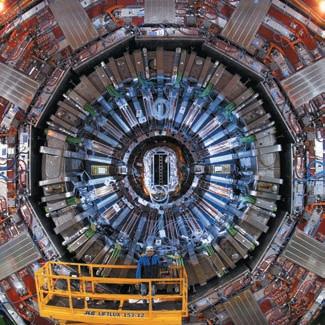
1 Two research laboratories. (a) According to legend, Galileo investigated falling bodies by dropping them from the Leaning Tower in Pisa, Italy, and he studied pendulum motion by observing the swinging of the chandelier in the adjacent cathedral. (b) The Large Hadron Collider (LHC) in Geneva, Switzerland, the world’s largest particle accelerator, is used to explore the smallest and most fundamental constituents of matter. This photo shows a portion of one of the LHC’s detectors (note the worker on the yellow platform).
(a)
(b)
Units, Physical Quantities, and Vectors
1 The Nature of Physics
Physics is an experimental science. Physicists observe the phenomena of nature and try to find patterns that relate these phenomena. These patterns are called physical theories or, when they are very well established and widely used, physical laws or principles.
CAUTION The meaning of the word “theory” Calling an idea a theory does not mean that it’s just a random thought or an unproven concept. Rather, a theory is an explanation of natural phenomena based on observation and accepted fundamental principles. An example is the well-established theory of biological evolution, which is the result of extensive research and observation by generations of biologists. ❙
To develop a physical theory, a physicist has to learn to ask appropriate questions, design experiments to try to answer the questions, and draw appropriate conclusions from the results. Figure 1shows two famous facilities used for physics experiments.
Legend has it that Galileo Galilei (1564–1642) dropped light and heavy objects from the top of the Leaning Tower of Pisa (Fig. 1a) to find out whether their rates of fall were the same or different. From examining the results of his experiments (which were actually much more sophisticated than in the legend), he made the inductive leap to the principle, or theory, that the acceleration of a falling body is independent of its weight.
The development of physical theories such as Galileo’s often takes an indirect path, with blind alleys, wrong guesses, and the discarding of unsuccessful theories in favor of more promising ones. Physics is not simply a collection of facts and principles; it is also the process by which we arrive at general principles that describe how the physical universe behaves.
No theory is ever regarded as the final or ultimate truth. The possibility always exists that new observations will require that a theory be revised or discarded. It is in the nature of physical theory that we can disprove a theory by finding behavior that is inconsistent with it, but we can never prove that a theory is always correct.
Getting back to Galileo, suppose we drop a feather and a cannonball. They certainly do not fall at the same rate. This does not mean that Galileo was wrong; it means that his theory was incomplete. If we drop the feather and the cannonball in a vacuum to eliminate the effects of the air, then they do fall at the same rate. Galileo’s theory has a range of validity: It applies only to objects for which the force exerted by the air (due to air resistance and buoyancy) is much less than the weight. Objects like feathers or parachutes are clearly outside this range.
Often a new development in physics extends a principle’s range of validity. Galileo’s analysis of falling bodies was greatly extended half a century later by Newton’s laws of motion and law of gravitation.
2 Solving Physics Problems
At some point in their studies, almost all physics students find themselves thinking, “I understand the concepts, but I just can’t solve the problems.” But in physics, truly understanding a concept means being able to apply it to a variety of problems. Learning how to solve problems is absolutely essential; you don’t know physics unless you can do physics.
How do you learn to solve physics problems? You will find Problem-Solving Strategies that offer techniques for setting up and solving problems efficiently and accurately. Following each Problem-Solving Strategy are one or more worked Examples that show these techniques in action. (The ProblemSolving Strategies will also steer you away from some incorrect techniques that you maybe tempted to use.) You’ll also find additional examples that aren’t associatedwith a particular Problem-Solving Strategy. In addition,
in this text you’ll find a Bridging Problem that uses more than one of the key ideas from the chapter. Study these strategies and problems carefully, and work through each example for yourself on a piece of paper.
Different techniques are useful for solving different kinds of physics problems, which is why this text offers dozens of Problem-Solving Strategies. No matter what kind of problem you’re dealing with, however, there are certain key steps that you’ll always follow. (These same steps are equally useful for problems in math, engineering, chemistry, and many other fields.) In this text we’ve organized these steps into four stages of solving a problem.
All of the Problem-Solving Strategies and Examples will follow these four steps. (In some cases we will combine the first two or three steps.) We encourage you to follow these same steps when you solve problems yourself. You may find it useful to remember the acronym I SEE—short for Identify, Set up, Execute, and Evaluate.
IDENTIFY the relevant concepts: Use the physical conditions stated in the problem to help you decide which physics concepts are relevant. Identify the target variables of the problem—that is, the quantities whose values you’re trying to find, such as the speed at which a projectile hits the ground, the intensity of a sound made by a siren, or the size of an image made by a lens. Identify the known quantities, as stated or implied in the problem. This step is essential whether the problem asks for an algebraic expression or a numerical answer.
SET UP the problem: Given the concepts you have identified and the known and target quantities, choose the equations that you’ll use to solve the problem and decide how you’ll use them. Make sure that the variables you have identified correlate exactly with those in the equations. If appropriate, draw a sketch of the situation described in the problem. (Graph paper, ruler, protractor, and compass will help you make clear, useful sketches.) As best you can,
Idealized Models
estimate what your results will be and, as appropriate, predict what the physical behavior of a system will be. The worked examples in this text include tips on how to make these kinds of estimates and predictions. If this seems challenging, don’t worry—you’ll get better with practice!
EXECUTE the solution: This is where you “do the math.” Study the worked examples to see what’s involved in this step.
EVALUATE your answer: Compare your answer with your estimates, and reconsider things if there’s a discrepancy. If your answer includes an algebraic expression, assure yourself that it represents what would happen if the variables in it were taken to extremes. For future reference, make note of any answer that represents a quantity of particular significance. Ask yourself how you might answer a more general or more difficult version of the problem you have just solved.
In everyday conversation we use the word “model” to mean either a small-scale replica, such as a model railroad, or a person who displays articles of clothing (or the absence thereof). In physics a model is a simplified version of a physical system that would be too complicated to analyze in full detail.
For example, suppose we want to analyze the motion of a thrown baseball (Fig. 2a). How complicated is this problem? The ball is not a perfect sphere (it has raised seams), and it spins as it moves through the air. Wind and air resistance influence its motion, the ball’s weight varies a little as its distance from the center of the earth changes, and so on. If we try to include all these things, the analysis gets hopelessly complicated. Instead, we invent a simplified version of the problem. We neglect the size and shape of the ball by representing it as a point object, or particle. We neglect air resistance by making the ball move in a vacuum, and we make the weight constant. Now we have a problem that is simple enough to deal with (Fig. 2b).
We have to overlook quite a few minor effects to make an idealized model, but we must be careful not to neglect too much. If we ignore the effects of gravity completely, then our model predicts that when we throw the ball up, it will go in a straight line and disappear into space. A useful model is one that simplifies a problem enough to make it manageable, yet keeps its essential features.
2 To simplify the analysis of (a) a baseball in flight, we use (b) an idealized model.
(a) A real baseball in flight
Baseball spins and has a complex shape.
Air resistance and wind exert forces on the ball.
Gravitational force on ball depends on altitude.
(b) An idealized model of the baseball
Baseball is treated as a point object (particle).
No air resistance.
Gravitational force on ball is constant.
Direction of motion
Direction of motion
3 The measurements used to determine (a) the duration of a second and (b) the length of a meter. These measurements are useful for setting standards because they give the same results no matter where they are made.
(a) Measuring the second
Microwave radiation with a frequency of exactly 9,192,631,770 cycles per second ...
Outermost electron
Cesium-133 atom
... causes the outermost electron of a cesium-133 atom to reverse its spin direction.
Cesium-133 atom
An atomic clock uses this phenomenon to tune microwaves to this exact frequency. It then counts 1 second for each 9,192,631,770 cycles.
(b) Measuring the meter
0:00 s0:01 s
Light source
Light travels exactly 299,792,458 m in 1 s.
The validity of the predictions we make using a model is limited by the validity of the model. For example, Galileo’s prediction about falling bodies (see Section 1) corresponds to an idealized model that does not include the effects of air resistance. This model works fairly well for a dropped cannonball, but not so well for a feather.
Idealized models play a crucial role in this text. Watch for them in discussions of physical theories and their applications to specific problems.
3 Standards and Units
As we learned in Section 1, physics is an experimental science. Experiments require measurements, and we generally use numbers to describe the results of measurements. Any number that is used to describe a physical phenomenon quantitatively is called a physical quantity. For example, two physical quantities that describe you are your weight and your height. Some physical quantities are so fundamental that we can define them only by describing how to measure them. Such a definition is called an operational definition. Two examples are measuring a distance by using a ruler and measuring a time interval by using a stopwatch. In other cases we define a physical quantity by describing how to calculate it from other quantities that we can measure. Thus we might define the average speed of a moving object as the distance traveled (measured with a ruler) divided by the time of travel (measured with a stopwatch).
When we measure a quantity, we always compare it with some reference standard. When we say that a Ferrari 458 Italia is 4.53 meters long, we mean that it is 4.53 times as long as a meter stick, which we define to be 1 meter long. Such a standard defines a unit of the quantity. The meter is a unit of distance, and the second is a unit of time. When we use a number to describe a physical quantity, we must always specify the unit that we are using; to describe a distance as simply “4.53” wouldn’t mean anything.
To make accurate, reliable measurements, we need units of measurement that do not change and that can be duplicated by observers in various locations. The system of units used by scientists and engineers around the world is commonly called “the metric system,” but since 1960 it has been known officially as the International System, or SI (the abbreviation for its French name, Système International).
Time
From 1889 until 1967, the unit of time was defined as a certain fraction of the mean solar day, the average time between successive arrivals of the sun at its highest point in the sky. The present standard, adopted in 1967, is much more precise. It is based on an atomic clock, which uses the energy difference between the two lowest energy states of the cesium atom. When bombarded by microwaves of precisely the proper frequency, cesium atoms undergo a transition from one of these states to the other. One second (abbreviated s) is defined as the time required for 9,192,631,770 cycles of this microwave radiation (Fig. 3a).
Length
(86Kr) Units, Physical Quantities, and Vectors
In 1960 an atomic standard for the meter was also established, using the wavelength of the orange-red light emitted by atoms of krypton in a glow discharge tube. Using this length standard, the speed of light in vacuum was measured to be 299,792,458 ms.In November 1983, the length standard was changed again so that the speed of light in vacuum was defined to be precisely
299,792,458 ms.Hence the new definition of the meter (abbreviated m) is the distance that light travels in vacuum in 1299,792,458second (Fig. 3b). This provides a much more precise standard of length than the one based on a wavelength of light.
Mass
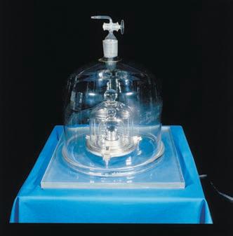
The standard of mass, the kilogram (abbreviated kg), is defined to be the mass of a particular cylinder of platinum–iridium alloy kept at the International Bureau of Weights and Measures at Sèvres, near Paris (Fig. 4). An atomic standard of mass would be more fundamental, but at present we cannot measure masses on an atomic scale with as much accuracy as on a macroscopic scale. The gram (which is not a fundamental unit) is 0.001 kilogram.
Unit Prefixes
Once we have defined the fundamental units, it is easy to introduce larger and smaller units for the same physical quantities. In the metric system these other units are related to the fundamental units (or, in the case of mass, to the gram) by multiples of 10 or Thus one kilometer is 1000 meters, and one centimeter is meter. We usually express multiples of 10 or in exponential notation: and so on. With this notation, and
cm = 10 - 2 m.
The names of the additional units are derived by adding a prefix to the name of the fundamental unit. For example, the prefix “kilo-,” abbreviated k, always means a unit larger by a factor of 1000; thus
4 The international standard kilogram is the metal object carefully enclosed within these nested glass containers.
Table 1 gives some examples of the use of multiples of 10 and their prefixes with the units of length, mass, and time. Figure 5shows how these prefixes are used to describe both large and small distances.
The British System
Finally, we mention the British system of units. These units are used only in the United States and a few other countries, and in most of these they are being replaced by SI units. British units are now officially defined in terms of SI units, as follows:
Length: 1 inch = 2.54 cm (exactly) 1 kilowatt = 1 kW = 10 3 watts = 10 3 W
Force: 1 pound = 4.448221615260 newtons (exactly)
Table 1 Some Units of Length, Mass, and Time
1 centimeter = 1 cm = 10 - 2 m 1 millimeter = 1 mm = 10 - 3 m 1 micrometer = 1 mm = 10 - 6 m 1 nanometer = 1 nm = 10 - 9 m
(a few times the size of the largest atom)
(size of some bacteria and living cells)
(diameter of the point of a ballpoint pen)
(diameter of your little finger)
1 kilometer = 1 km = 10 3 m
(a 10-minute walk)
(mass of a very small dust particle)
(mass of a grain of salt)
(mass of a paper clip)
(time for light to travel 0.3 m)
(time for space station to move 8 mm)
(time for sound to travel 0.35 m)
Units, Physical Quantities, and Vectors
5 Some typical lengths in the universe. (f ) is a scanning tunneling microscope image of atoms on a crystal surface; (g) is an artist’s impression.
(a)1026 m Limit of the observable universe
R. Williams (STScI), the HDF-STeam, and NASA
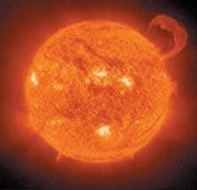
(b)1011 m Distance to the sun
(c)107 m Diameter of the earth
SOHO (ESA& NASA) Courtesy of NASA/JPL/ Caltech
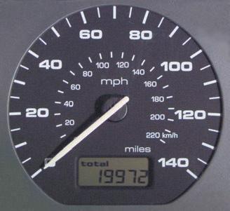
6 Many everyday items make use of both SI and British units. An example is this speedometer from a U.S.-built automobile, which shows the speed in both kilometers per hour (inner scale) and miles per hour (outer scale).
Purdue University. Veeco Instruments, Inc. SPL/PhotoResearchers, Inc.
(f)10 10 m Radius of an atom
(g)10 14 m Radius of an atomic nucleus
The newton, abbreviated N, is the SI unit of force. The British unit of time is the second, defined the same way as in SI. In physics, British units are used only in mechanics and thermodynamics; there is no British system of electrical units.
In this text we use SI units for all examples and problems, but we occasionally give approximate equivalents in British units. As you do problems using SI units, you may also wish to convert to the approximate British equivalents if they are more familiar to you (Fig. 6). But you should try to think in SI units as much as you can.
4 Unit Consistency and Conversions
We use equations to express relationships among physical quantities, represented by algebraic symbols. Each algebraic symbol always denotes both a number and a unit. For example, d might represent a distance of 10 m, t a time of 5 s, and a speed of
An equation must always be dimensionally consistent. You can’t add apples and automobiles; two terms may be added or equated only if they have the same units. For example, if a body moving with constant speed travels a distance d in a time t, these quantities are related by the equation
If d is measured in meters, then the product must also be expressed in meters. Using the above numbers as an example, we may write
Because the unit on the right side of the equation cancels the unit s, the product has units of meters, as it must. In calculations, units are treated just like algebraic symbols with respect to multiplication and division.
CAUTION Always use units in calculations When a problem requires calculations using numbers with units, always write the numbers with the correct units and carry the units through the calculation as in the example above. This provides a very useful check. If at some stage in a calculation you find that an equation or an expression has inconsistent units, you know you have made an error somewhere. In this text we will always carry units through all calculations, and we strongly urge you to follow this practice when you solve problems.
IDENTIFY the relevant concepts: In most cases, it’s best to use the fundamental SI units (lengths in meters, masses in kilograms, and times in seconds) in every problem. If you need the answer to be in a different set of units (such as kilometers, grams, or hours), wait until the end of the problem to make the conversion.
SET UP the problem and EXECUTE the solution: Units are multiplied and divided just like ordinary algebraic symbols. This gives us an easy way to convert a quantity from one set of units to another: Express the same physical quantity in two different units and form an equality.
For example, when we say that we don’t mean that the number 1 is equal to the number 60; rather, we mean that 1 min represents the same physical time interval as 60 s. For this reason, the ratio equals 1, as does its reciprocal
We may multiply a quantity by either of these 160 s2> 11 min2
Example 1 Converting speed units
The world land speed record is 763.0 mih, set on October 15, 1997, by Andy Green in the jet-engine car Thrust SSC. Express this speed in meters per second.
SOLUTION
1 h = 3600 s.
IDENTIFY, SET UP,and EXECUTE: We need to convert the units of a speed from mih to We must therefore find unit multipliers that relate (i) miles to meters and (ii) hours to seconds. We can findthe equalities and We set up the conversion as follows, which ensures that all the desired cancellations by division take place:
Example 2
Converting volume units
The world’s largest cut diamond is the First Star of Africa (mounted in the British Royal Sceptre and kept in the Tower of London). Its volume is 1.84 cubic inches. What is its volume in cubic centimeters? In cubic meters?
SOLUTION
IDENTIFY, SET UP, andEXECUTE: Here we are to convert the units of a volume from cubic inches to both cubic centimeters and cubic meters Recall that from which we obtain . We then have
factors (which we call unit multipliers) without changing that quantity’s physical meaning. For example, to find the number of seconds in 3 min, we write
EVALUATE your answer: If you do your unit conversions correctly, unwanted units will cancel, as in the example above. If, instead, you had multiplied 3 min by your result would have been the nonsensical . To be sure you convert units properly, you must write down the units at all stages of the calculation. Finally, check whether your answer is reasonable. For example, the result is reasonable because the second is a smaller unit than the minute, so there are more seconds than minutes in the same time interval. 3 min = 180 s 1 20 min2> s 11 min2>160 s2, 3 min = 13 min2a 60 s
EVALUATE: Green’s was the first supersonic land speed record (the speed of sound in air is about 340 ms). This example shows a useful rule of thumb: Aspeed expressed in ms is a bit less than half the value expressed in mih, and a bit less than one-third the value expressed in kmh. For example, a normal freeway speed is about and a typical walking speed is about 1.4 m> s = 3.1
Recall that so
EVALUATE: Following the pattern of these conversions, you can show that and that . These approximate unit conversions may be useful for future reference. 1 m3 L 60,000 in.3 1 in.3 L 16 cm3
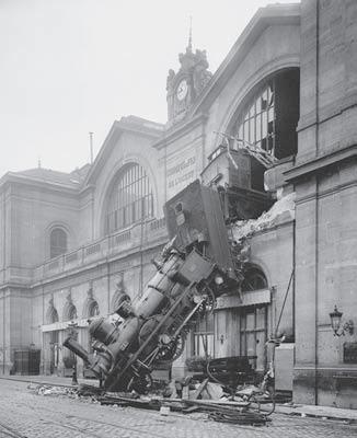
7 This spectacular mishap was the result of a very small percent error—traveling a few meters too far at the end of a journey of hundreds of thousands of meters.
Table 2 Using Significant Figures
Multiplication or division:
Result may have no more significant figures than thestarting number with the fewest significant figures:
0.745 * 2.2 3.885 = 0.42
1.32578 * 107 * 4.11 * 10 - 3 = 5.45 * 104
Addition or subtraction:
Number of significant figures is determined by the starting number with thelargest uncertainty (i.e., fewest digits to the right of the decimal point):
27.153 + 138.2 - 11.74 = 153.6
8 Determining the value of from the circumference and diameter of a circle. p
5
Uncertainty and Significant Figures
Measurements always have uncertainties. If you measure the thickness of the cover of a hardbound version of a book using an ordinary ruler, your measurement is reliable only to the nearest millimeter, and your result will be 3 mm. It would be wrong to state this result as 3.00 mm; given the limitations of the measuring device, you can’t tell whether the actual thickness is 3.00 mm, 2.85 mm, or 3.11 mm. But if you use a micrometer caliper, a device that measures distances reliably to the nearest 0.01 mm, the result will be 2.91 mm. The distinction between these two measurements is in their uncertainty. The measurement using the micrometer caliper has a smaller uncertainty; it’s a more accurate measurement. The uncertainty is also called the error because it indicates the maximum difference there is likely to be between the measured value and the true value. The uncertainty or error of a measured value depends on the measurement technique used.
We often indicate the accuracy of a measured value—that is, how close it is likely to be to the true value—by writing the number, the symboland a second number indicating the uncertainty of the measurement. If the diameter of a steel rod is given as this means that the true value is unlikely to be less than 56.45 mm or greater than 56.49 mm. In a commonly used shorthand notation, the number means The numbers in parentheses show the uncertainty in the final digits of the main number.
We can also express accuracy in terms of the maximum likely fractional error or percent error (also called fractional uncertainty and percent uncertainty). A resistor labeled probably has a true resistance that differs from 47 ohms by no more than 10% of 47 ohms—that is, by about 5 ohms. The resistance is probably between 42 and 52 ohms. For the diameter of the steel rod given above, the fractional error is or about 0.0004; the percent error is or about 0.04%. Even small percent errors can sometimes be very significant (Fig. 7).
In many cases the uncertainty of a number is not stated explicitly. Instead, the uncertainty is indicated by the number of meaningful digits, or significant figures, in the measured value. We gave the thickness of the cover of a book as 2.91 mm, which has three significant figures. By this we mean that the first two digits are known to be correct, while the third digit is uncertain. The last digit is in the hundredths place, so the uncertainty is about 0.01 mm. Two values with the same number of significant figures may have different uncertainties; a distance given as 137 km also has three significant figures, but the uncertainty is about 1 km.
When you use numbers that have uncertainties to compute other numbers, the computed numbers are also uncertain. When numbers are multiplied or divided, the number of significant figures in the result can be no greater than in the factor with the fewest significant figures. For example, When we add and subtract numbers, it’s the location of the decimal point that matters, not the number of significant figures. For example, Although 123.62 has an uncertainty of about 0.01, 8.9 has an uncertainty of about 0.1. So their sum has an uncertainty of about 0.1 and should be written as 132.5, not 132.52. Table 2 summarizes these rules for significant figures.
The measured values have only three significant figures, so their calculated ratio (p) also has only three significant figures.
As an application of these ideas, suppose you want to verify the value of the ratio of the circumference of a circle to its diameter. The true value of this ratio to ten digits is 3.141592654. To test this, you draw a large circle and measure its circumference and diameter to the nearest millimeter, obtaining the values 424 mm and 135 mm (Fig. 8). You punch these into your calculator and obtain the quotient . This may seem to disagree with the true value of but keep in mind that each of your measurements has three significant figures, so your measured value of can have only three significant figures. It should be stated simply as 3.14. Within the limit of three significant figures, your value does agree with the true value. p p, 1424 mm2>1135 mm2 = 3.140740741
Units, Physical Quantities, and Vectors
In the examples and problems in this text we usually give numerical values with three significant figures, so your answers should usually have no more than three significant figures. (Many numbers in the real world have even less accuracy. An automobile speedometer, for example, usually gives only two significant figures.) Even if you do the arithmetic with a calculator that displays ten digits, it would be wrong to give a ten-digit answer because it misrepresents the accuracy of the results. Always round your final answer to keep only the correct number of significant figures or, in doubtful cases, one more at most. In Example 1 it would have been wrong to state the answer as
m> s.
Note that when you reduce such an answer to the appropriate number of significant figures, you must round, not truncate. Your calculator will tell you that the ratio of 525 m to 311 m is 1.688102894; to three significant figures, this is 1.69, not 1.68.
When we calculate with very large or very small numbers, we can show significant figures much more easily by using scientific notation, sometimes called powers-of-10 notation. The distance from the earth to the moon is about 384,000,000 m, but writing the number in this form doesn’t indicate the number of significant figures. Instead, we move the decimal point eight places to the left (corresponding to dividing by 108)and multiply by that is,
In this form, it is clear that we have three significant figures. The number also has three significant figures, even though two of them are zeros. Note that in scientific notation the usual practice is to express the quantity as a number between 1 and 10 multiplied by the appropriate power of 10.
When an integer or a fraction occurs in a general equation, we treat that number as having no uncertainty at all. For example, in the equation the coefficient 2 is exactly 2. We can consider this coefficient as having an infinite number of significant figures
The same is true of the exponent 2 in and Finally, let’s note that precision is not the same as accuracy. Acheap digital watch that gives the time as 10:35:17 A.M.is very precise (the time is given to the second), but if the watch runs several minutes slow, then this value isn’t very accurate. On the other hand, a grandfather clock might be very accurate (that is, display the correct time), but if the clock has no second hand, it isn’t very precise. Ahigh-quality measurement is both precise and accurate. v0x 2 vx 2
Example 3 Significant figures in multiplication
The rest energy E of an object with rest mass m is given by Einstein’s famous equation , where c is the speed of light in vacuum. Find E for an electron for which (to three significant figures) . The SI unit for E is the joule (J);
1 J = 1 kg # m2> s 2 m = 9.11 * 10 - 31 kg E = mc 2
SOLUTION
IDENTIFY andSET UP: Our target variable is the energy E. We are given the value of the mass m; from Section 3 the speed of light is
Since the value of m was given to only three significant figures, we must round this to
10 - 19 J, E = 8.19 * 10 - 14 kg m2> s 2 = 8.19 * 10 - 14 J
EVALUATE: While the rest energy contained in an electron may seem ridiculously small, on the atomic scale it is tremendous. Compare our answer to the energy gained or lost by a single atom during a typical chemical reaction. The rest energy of an electron is about 1,000,000 times larger!
EXECUTE: Substituting the values of m and c into Einstein’s equation, we find
E = 19.11 * 10 - 31 kg212.99792458 * 108 m> s22 c = 2.99792458 * 10 8 m> s.
= 19.11212.9979245822110 - 312110822 kg # m2> s2
= 181.8765967821103 - 31 + 12 * 8242 kg m2> s2
= 8.187659678 * 10 - 14 kg # m2> s2
PhET: Estimation
Units, Physical Quantities, and Vectors
Test Your Understanding of Section 5 The density of a material is equal to its mass divided by its volume. What is the density of a rock of mass 1.80 kg and volume (i) (ii) (iii) (iv) (v) any of these—all of these answers are mathematically equivalent. ❙ 3.000 * 10 3 kg > m3; 3.00 * 10 3 kg > m3; 10 3 kg > m3; 3.0 * 3 * 10 3 kg> m3; 6.0 * 10 - 4 m3? (in kg> m3)
6
Estimates and Orders of Magnitude
We have stressed the importance of knowing the accuracy of numbers that represent physical quantities. But even a very crude estimate of a quantity often gives us useful information. Sometimes we know how to calculate a certain quantity, but we have to guess at the data we need for the calculation. Or the calculation might be too complicated to carry out exactly, so we make some rough approximations. In either case our result is also a guess, but such a guess can be useful even if it is uncertain by a factor of two, ten, or more. Such calculations are often called order-of-magnitude estimates. The great Italian-American nuclear physicist Enrico Fermi (1901–1954) called them “back-of-the-envelope calculations.”
Exercises 16 through 25 at the end of this chapter are of the estimating, or order-of-magnitude, variety. Most require guesswork for the needed input data. Don’t try to look up a lot of data; make the best guesses you can. Even when they are off by a factor of ten, the results can be useful and interesting.
You are writing an adventure novel in which the hero escapes across the border with a billion dollars’worth of gold in his suitcase. Could anyone carry that much gold? Would it fit in a suitcase?
SOLUTION
IDENTIFY, SET UP, andEXECUTE: Gold sells for around $400 an ounce. (The price has varied between $200 and $1000 over the past decade or so.) An ounce is about 30 grams; that’s worth remembering. So ten dollars’worth of gold has a mass of ounce, or around one gram. Abillion dollars’worth of gold 11092
is a hundred million grams, or a hundred thousand kilograms. This corresponds to a weight in British units of around 200,000 lb, or 100 tons. No human hero could lift that weight!
Roughly what is the volume of this gold? The density of gold is much greater than that of water , or ; if its density is 10 times that of water, this much gold will have a volume of , many times the volume of a suitcase.
EVALUATE: Clearly your novel needs rewriting. Try the calculation again with a suitcase full of five-carat (1-gram) diamonds, each worth $100,000. Would this work? 10 m3
Application Scalar Temperature, Vector Wind
This weather station measures temperature, a scalar quantity that can be positive or negative (say, ) but has no direction. It also measures wind velocity, which is a vector quantity with both magnitude and direction (for example, 15 km/h from the west).
+ 20°C or - 5°C
Test Your Understanding of Section 6 Can you estimate the total number of teeth in all the mouths of everyone (students, staff, and faculty) on your campus? (Hint: How many teeth are in your mouth? Count them!) ❙
7 Vectors and Vector Addition
Some physical quantities, such as time, temperature, mass, and density, can be described completely by a single number with a unit. But many other important quantities in physics have a direction associated with them and cannot be described by a single number. Asimple example is describing the motion of an airplane: We must say not only how fast the plane is moving but also in what direction. The speed of the airplane combined with its direction of motion together constitute a quantity called velocity. Another example is force, which in physics means a push or pull exerted on a body. Giving a complete description of a force means describing both how hard the force pushes or pulls on the body and the direction of the push or pull.
Example 4 An order-of-magnitude estimate
Scott Bauer -
When a physical quantity is described by a single number, we call it a scalar quantity. In contrast, a vector quantity has both a magnitude (the “how much” or “how big” part) and a direction in space. Calculations that combine scalar quantities use the operations of ordinary arithmetic. For example, or However, combining vectors requires a different set of operations.
4 * 2 s = 8 s. 6 kg + 3 kg = 9 kg,
To understand more about vectors and how they combine, we start with the simplest vector quantity, displacement. Displacement is simply a change in the position of an object. Displacement is a vector quantity because we must state not only how far the object moves but also in what direction. Walking 3 km north from your front door doesn’t get you to the same place as walking 3 km southeast; these two displacements have the same magnitude but different directions.
We usually represent a vector quantity such as displacement by a single letter, such as in Fig. 9a. In this text we always print vector symbols in boldface italic type with an arrow above them. We do this to remind you that vector quantities have different properties from scalar quantities; the arrow is a reminder that vectors have direction. When you handwrite a symbol for a vector, always write it with an arrow on top. If you don’t distinguish between scalar and vector quantities in your notation, you probably won’t make the distinction in your thinking either, and hopeless confusion will result.
We always draw a vector as a line with an arrowhead at its tip. The length of the line shows the vector’s magnitude, and the direction of the line shows the vector’s direction. Displacement is always a straight-line segment directed from the starting point to the ending point, even though the object’s actual path may be curved (Fig. 9b). Note that displacement is not related directly to the total distance traveled. If the object were to continue on past and then return to the displacement for the entire trip would be zero (Fig. 9c).
If two vectors have the same direction, they are parallel. If they have the same magnitude and the same direction, they are equal, no matter where they are located in space. The vector from point to point in Fig. 10has the same length and direction as the vector from to These two displacements are equal, even though they start at different points. We write this as in Fig. 10; the boldface equals sign emphasizes that equality of two vector quantities is not the same relationship as equality of two scalar quantities. Two vector quantities are equal only when they have the same magnitude and the same direction.
The vector in Fig. 10, however, is not equal to because its direction is opposite to that of We define the negative of a vector as a vector having the same magnitude as the original vector but the opposite direction. The negative of vector quantity is denoted as and we use a boldface minus sign to emphasize the vector nature of the quantities. If is 87 m south, then is 87 m north. Thus we can write the relationship between and in Fig. 10as or When two vectors and have opposite directions, whether their magnitudes are the same or not, we say that they are antiparallel.
We usually represent the magnitude of a vector quantity (in the case of a displacement vector, its length) by the same letter used for the vector, but in light italic type with no arrow on top. An alternative notation is the vector symbol with vertical bars on both sides:
Magnitude of A S 2 = A = A S
The magnitude of a vector quantity is a scalar quantity (a number) and is always positive. Note that a vector can never be equal to a scalar because they are different kinds of quantities. The expression is just as wrong as
When drawing diagrams with vectors, it’s best to use a scale similar to those used for maps. For example, a displacement of 5 km might be represented in a diagram by a vector 1 cm long, and a displacement of 10 km by a vector 2 cm long. In a diagram for velocity vectors, a vector that is 1 cm long might represent “2 oranges = 3 apples”
9 Displacement as a vector quantity. A displacement is always a straight-line segment directed from the starting point to the ending point, even if the path is curved.
We represent a displacement by an arrow pointing in the direction of displacement.
Ending position: P2
Displacement A
Starting position: P1
Handwritten notation:
Displacement depends only on the starting and ending positions—not on the path taken.
Path taken
Total displacement for a round trip is 0, regardless of the distance traveled.
10 The meaning of vectors that have the same magnitude and the same or opposite direction.
S
Displacements A and A are equal because they have the same length and direction.
Displacement B has the same magnitude as A but opposite direction; B is the negative of A
(a)
(b)
(c)
11 Three ways to add two vectors. As shown in (b) , the order in vector addition doesn’t matter; vector addition is commutative.
(a) We can add two vectors by placing them head to tail.
(b) Adding them in reverse order gives the same result.
a velocity of magnitude 5 ms.A velocity of 20 mswould then be represented by a vector 4 cm long.
Vector Addition and Subtraction
Suppose a particle undergoes a displacement followed by a second displacement . The final result is the same as if the particle had started at the same initial point and undergone a single displacement (Fig. 11a). We call displacement the vector sum, or resultant, of displacements and We express this relationship symbolically as
(2)
The boldface plus sign emphasizes that adding two vector quantities requires a geometrical process and is not the same operation as adding two scalar quantities such as In vector addition we usually place the tail of the second vector at the head, or tip, of the first vector (Fig. 11a).
If we make the displacements and in reverse order, with first and second, the result is the same (Fig. 11b). Thus
(c) We can also add them by constructing a parallelogram.
12 (a) Only when two vectors and are parallel does the magnitude of their sum equal the sum of their magnitudes: (b) When and are antiparallel, the magnitude of their sum equals the difference of their magnitudes: C = A - B
(a) The sum of two parallel vectors
(b) The sum of two antiparallel vectors
(3)
This shows that the order of terms in a vector sum doesn’t matter. In other words, vector addition obeys the commutative law.
Figure 11c shows another way to represent the vector sum: If vectors and are both drawn with their tails at the same point, vector is the diagonal of a parallelogram constructed with and as two adjacent sides.
CAUTION Magnitudes in vector addition It’s a common error to conclude that if then the magnitude C should equal the magnitude A plus the magnitude B. In general, this conclusion is wrong; for the vectors shown in Fig. 11, you can see that The magnitude of depends on the magnitudes of and and on the angle between and . Only in the special case in which and are parallel is the magnitude of equal to the sum of the magnitudes of and (Fig. 12a). When the vectors are antiparallel (Fig. 12b), the magnitude of equals the difference of the magnitudes of and Be careful about distinguishing between scalar and vector quantities, and you’ll avoid making errors about the magnitude of a vector sum. ❙
When we need to add more than two vectors, we may first find the vector sum of any two, add this vectorially to the third, and so on. Figure 13a shows three vectors and In Fig. 13b we first add and to give a vector sum we then add vectors and by the same process to obtain the vector sum
13 Several constructions for finding the vector sum
(a) To find the sum of these three vectors ...
(b) we could add A and B to get D and then add C to D to get the final sum (resultant) R,