Where can buy Introduction to linear algebra for science and engineering 2nd edition (student editio
Edition) Edition Daniel Norman
Visit to download the full and correct content document: https://ebookmass.com/product/introduction-to-linear-algebra-for-science-and-engine ering-2nd-edition-student-edition-edition-daniel-norman/
More products digital (pdf, epub, mobi) instant download maybe you interests ...
Introduction to Linear Algebra for Science and Engineering 2nd Edition (Student Edition) Edition
Published by Pearson Upper Saddle River, New Jersey 07458
All rights reserved. No part of this book may be reproduced, in any form or by any means, without permission in writing from the publisher.
This special edition published in cooperation with Pearson Learning Solutions.
All trademarks, service marks, registered trademarks, and registered service marks are the property of their respective owners and are used herein for identification purposes only.
Pearson Learning Solutions, 501 Boylston Street, Suite 900, Boston, MA 02116
A Pearson Education Company www.pearsoned.com
A Note to Students vi
A Note to Instructors viii
Chapter 1 Euclidean Vector Spaces 1
1.1 Vectors in JR2 and JR3 1
The Vector Equation of a Line in JR2 5
Vectors and Lines in JR3 9
1.2 Vectors in JRll 14
Addition and Scalar Multiplication of Vectors in JR11 15
Subspaces 16
Spanning Sets and Linear Independence 18
Surfaces in Higher Dimensions 24
1.3 Length and Dot Products 28
Length and Dot Products in JR2, and JR3 28
Length and Dot Product in JR11 31
The Scalar Equation of Planes and Hyperplanes 34
1.4 Projections and Minimum Distance 40 Projections 40
The Perpendicular Part 43
Some Properties of Projections 44
Minimum Distance 44
1.5 Cross-Products and Volumes 50
Cross-Products 50
The Length of the Cross-Product 52
Some Problems on Lines, Planes, and Distances 54
Chapter 2 Systems of Linear Equations 63
2.1 Systems of Linear Equations and Elimination 63
The Matrix Representation of a System of Linear Equations 69 Row Echelon Form 73
Consistent Systems and Unique Solutions 75
Some Shortcuts and Some Bad Moves 76
A Word Problem 77
A Remark on Computer Calculations 78
2.2 Reduced Row Echelon Form, Rank, and Homogeneous Systems 83
Rank of a Matrix 85
Homogeneous Linear Equations 86
2.3 Application to Spanning and Linear Independence 91
Spanning Problems 91
Linear Independence Problems 95
Bases of Subspaces 97
2.4 Applications of Systems of Linear Equations 102
Resistor Circuits in Electricity 102
Planar Trusses 105
Linear Programming 107
Chapter 3 Matrices, Linear Mappings, and Inverses 115
3.1 Operations on Matrices 115
Equality, Addition, and Scalar Multiplication of Matrices 115
The Transpose of a Matrix 120
An Introduction to Matrix Multiplication 121
Identity Matrix 126
Block Multiplication 127
3.2 Matrix Mappings and Linear Mappings 131
Matrix Mappings 131
Linear Mappings 134
Is Every Linear Mapping a Matrix Mapping? 136 Compositions and Linear Combinations of Linear Mappings 139
3.3 Geometrical Transformations 143
Rotations in the Plane 143
Rotation Through Angle e About the X3-axis in JR3 145
3.4 Special Subspaces for Systems and Mappings: Rank Theorem 150
Solution Space and Nullspace 150
Solution Set of Ax = b 152
Range of L and Columnspace of A 153 Rowspace of A 156
Bases for Row(A), Col(A), and Null(A) 157
A Summary of Facts About Rank 162
3.5 Inverse Matrices and Inverse Mappings 165
A Procedure for Finding the Inverse of a Matrix 167
Some Facts About Square Matrices and Solutions of Linear Systems 168
Inverse Linear Mappings 170
3.6 Elementary Matrices 175
3.7 LU-Decomposition 181
Solving Systems with the LU-Decomposition 185
A Comment About Swapping Rows 187
Chapter 4 Vector Spaces 193
4.1 Spaces of Polynomials 193
Addition and Scalar Multiplication of Polynomials 193
4.2 Vector Spaces 197
Vector Spaces 197
Subspaces 201
4.3 Bases and Dimensions 206 Bases 206
Obtaining a Basis from an Arbitrary Finite Spanning Set 209
Dimension 211
Extending a Linearly Independent Subset to a Basis 213
4.4 Coordinates with Respect to a Basis 218
4.5 General Linear Mappings 226
4.6 Matrix of a Linear Mapping 235
The Matrix of L with Respect to the Basis B 235
Change of Coordinates and Linear Mappings 240
4.7 Isomorphisms of Vector Spaces 246
Chapter 5 Determinants 255
5.1 Determinants in Terms of Cofactors 255
The 3 x 3 Case 256
5.2 Elementary Row Operations and the Determinant 264
The Determinant and Invertibility 270
Determinant of a Product 270
5.3 Matrix Inverse by Cofactors and Cramer's Rule 274
Cramer's Rule 276
5.4 Area, Volume, and the Determinant 280 Area and the Determinant 280
The Determinant and Volume 283
Chapter 6 Eigenvectors
and Diagonalization 289
6.1 Eigenvalues and Eigenvectors 289
Eigenvalues and Eigenvectors of a Mapping 289
Eigenvalues and Eigenvectors of a Matrix 291
Finding Eigenvectors and Eigenvalues 291
6.2 Diagonalization 299
Some Applications of Diagonalization 303
6.3 Powers of Matrices and the Markov Process 307
Systems of Linear Difference Equations 312
The Power Method of Determining Eigenvalues 312
6.4 Diagonalization and Differential Equations 315
A Practical Solution Procedure 317
General Discussion 317
Chapter 7 Orthonormal Bases 321
7.1 Orthonormal Bases and Orthogonal Matrices 321
Orthonormal Bases 321
Coordinates with Respect to an Orthonormal Basis 323
Change of Coordinates and Orthogonal Matrices 325
A Note on Rotation Transformations and Rotation of Axes in JR.2 329
7.2 Projections and the Gram-Schmidt Procedure 333
Projections onto a Subspace 333
The Gram-Schmidt Procedure 337
7.3 Method of Least Squares 342
Overdetermined Systems 345
7.4 Inner Product Spaces 348
Inner Product Spaces 348
7.5 Fourier Series 354 b
The Inner Product J f(x)g(x) dx 354 a Fourier Series 355
Chapter 8 Symmetric Matrices and Quadratic Forms 363
8.1 Diagonalization ofSymmetric Matrices 363
The Principal Axis Theorem 366
8.2 Quadratic Forms 372
Quadratic Forms 372
Classifications of Quadratic Forms 376
8.3 Graphs of Quadratic Forms 380
Graphs of Q(x) = k in JR.3 385
8.4 Applications of Quadratic Forms 388
Small Deformations 388
The Inertia Tensor 390
Chapter 9 Complex Vector Spaces 395
9.1 Complex Numbers 395
The Arithmetic of Complex Numbers 395
The Complex Conjugate and Division 397
Roots of Polynomial Equations 398
The Complex Plane 399
Polar Form 399
Powers and the Complex Exponential 402
n-th Roots 404
9.2 Systems with Complex Numbers 407
Complex Numbers in Electrical Circuit Equations 408
9.3 Vector Spaces over C 411
Linear Mappings and Subspaces 413
Complex Multiplication as a Matrix Mapping 415
9.4 Eigenvectors in Complex Vector Spaces 417
Complex Characteristic Roots of a Real Matrix and a Real Canonical Form 418
The Case of a 2 x 2 Matrix 420
The Case of a 3 x 3 Matrix 422
9.5 Inner Products in Complex Vector Spaces 425
Properties of Complex Inner Products 426
The Cauchy-Schwarz and Triangle Inequalities 426
Orthogonality in C" and Unitary Matrices 429
9.6 Hermitian Matrices and Unitary
Diagonalization 432
Appendix A Exercises Answers to Mid-Section 439
Appendix B Answers to Practice Problems and Chapter Quizzes 465
Index 529
A Note to Students Linear Algebra-What Is It?
Linear algebra is essentially the study of vectors, matrices, and linear mappings. Although many pieces of linear algebra have been studied for many centuries, it did not take its current form until the mid-twentieth century. It is now an extremely important topic in mathematics because of its application to many different areas.
Most people who have learned linear algebra and calculus believe that the ideas of elementary calculus (such as limit and integral) are more difficult than those of introductory linear algebra and that most problems in calculus courses are harder than those in linear algebra courses. So, at least by this comparison, linear algebra is not hard. Still, some students find learning linear algebra difficult. I think two factors contribute to the difficulty students have.
First, students do not see what linear algebra is good for. This is why it is important to read the applications in the text; even if you do not understand them completely, they will give you some sense of where linear algebra fits into the broader picture.
Second, some students mistakenly see mathematics as a collection of recipes for solving standard problems and are uncomfortable with the fact that linear algebra is "abstract" and includes a lot of "theory." There will be no long-term payoff in simply memorizing these recipes, however; computers carry them out far faster and more accurately than any human can. That being said, practising the procedures on specific examples is often an important step toward much more important goals: understanding the concepts used in linear algebra to formulate and solve problems and learning to interpret the results of calculations. Such understanding requires us to come to terms with some theory. In this text, many of our examples will be small. However, as you work through these examples, keep in mind that when you apply these ideas later, you may very well have a million variables and a million equations. For instance, Google's PageRank system uses a matrix that has 25 billion columns and 25 billion rows; you don't want to do that by hand! When you are solving computational problems, always try to observe how your work relates to the theory you have learned.
Mathematics is useful in so many areas because it is abstract: the same good idea can unlock the problems of control engineers, civil engineers, physicists, social scientists, and mathematicians only because the idea has been abstracted from a particular setting. One technique solves many problems only because someone has established a theory of how to deal with these kinds of problems. We use definitions to try to capture important ideas, and we use theorems to summarize useful general facts about the kind of problems we are studying. Proofs not only show us that a statement is true; they can help us understand the statement, give us practice using important ideas, and make it easier to learn a given subject. In particular, proofs show us how ideas are tied together so we do not have to memorize too many disconnected facts.
Many of the concepts introduced in linear algebra are natural and easy, but some may seem unnatural and "technical" to beginners. Do not avoid these apparently more difficult ideas; use examples and theorems to see how these ideas are an essential part of the story of linear algebra. By learning the "vocabulary" and "grammar" of linear algebra, you will be equipping yourself with concepts and techniques that mathematicians, engineers, and scientists find invaluable for tackling an extraordinarily rich variety of problems.
Linear Algebra-Who Needs It?
Mathematicians
Linear algebra and its applications are a subject of continuing research. Linear algebra is vital to mathematics because it provides essential ideas and tools in areas as diverse as abstract algebra, differential equations, calculus of functions of several variables, differential geometry, functional analysis, and numerical analysis.
Engineers
Suppose you become a control engineer and have to design or upgrade an automatic control system. The system may be controlling a manufacturing process or perhaps an airplane landing system. You will probably start with a linear model of the system, requiring linear algebra for its solution. To include feedback control, your system must take account of many measurements (for the example of the airplane, position, velocity, pitch, etc.), and it will have to assess this information very rapidly in order to determine the correct control responses. A standard part of such a control system is a Kalman-Bucy filter, which is not so much a piece of hardware as a piece of mathematical machinery for doing the required calculations. Linear algebra is an essential part of the Kalman-Bucy filter.
If you become a structural engineer or a mechanical engineer, you may be concerned with the problem of vibrations in structures or machinery. To understand the problem, you will have to know about eigenvalues and eigenvectors and how they determine the normal modes of oscillation. Eigenvalues and eigenvectors are some of the central topics in linear algebra.
An electrical engineer will need linear algebra to analyze circuits and systems; a civil engineer will need linear algebra to determine internal forces in static structures and to understand principal axes of strain.
In addition to these fairly specific uses, engineers will also find that they need to know linear algebra to understand systems of differential equations and some aspects of the calculus of functions of two or more variables. Moreover, the ideas and techniques of linear algebra are central to numerical techniques for solving problems of heat and fluid flow, which are major concerns in mechanical engineering. And the ideas of Jjnear algebra underjje advanced techniques such as Laplace transforms and Fourier analysis.
Physicists
Linear algebra is important in physics, partly for the reasons described above. In addition, it is essential in applications such as the inertia tensor in general rotating motion. Linear algebra is an absolutely essential tool in quantum physics (where, for example, energy levels may be determined as eigenvalues of linear operators) and relativity (where understanding change of coordinates is one of the central issues).
Life and Social Scientists
Input/output models, described by matrices, are often used in economics, and similar ideas can be used in modelling populations where one needs to keep track of subpopulations (generations, for example, or genotypes). In all sciences, statistical analysis of data is of great importance, and much of this analysis uses Jjnear algebra; for example, the method of least squares (for regression) can be understood in terms of projections in linear algebra.
Managers
A manager in industry will have to make decisions about the best allocation of resources: enormous amounts of computer time around the world are devoted to linear programming algorithms that solve such allocation problems. The same sorts of techniques used in these algorithms play a role in some areas of mine management. Linear algebra is essential here as well.
So who needs linear algebra? Almost every mathematician, engineer, or scientist will .find linear algebra an important and useful tool.
Will these applications be explained in this book?
Unfortunately, most of these applications require too much specialized background to be included in a first-year linear algebra book. To give you an idea of how some of these concepts are applied, a few interesting applications are briefly covered in sections 1.4, 1.5, 2.4, 5.4, 6.3, 6.4, 7.3, 7.5, 8.3, 8.4, and 9.2. You will get to see many more applications of linear algebra in your future courses.
A Note to Instructors
Welcome to the second edition of Introduction to Linear Algebra for Science and Engineering. It has been a pleasure to revise Daniel Norman's first edition for a new generation of students and teachers. Over the past several years, I have read many articles and spoken to many colleagues and students about the difficulties faced by teachers and learners of linear algebra. In particular, it is well known that students typically find the computational problems easy but have great difficulty in understanding the abstract concepts and the theory. Inspired by this research, I developed a pedagogical approach that addresses the most common problems encountered when teaching and learning linear algebra. I hope that you will find this approach to teaching linear algebra as successful as I have.
Changes to the Second Edition
• Several worked-out examples have been added, as well as a variety of midsection exercises (discussed below).
• Vectors in JR.11 are now always represented as column vectors and are denoted with the normal vector symbol 1. Vectors in general vector spaces are still denoted in boldface.
• Some material has been reorganized to allow students to see important concepts early and often, while also giving greater flexibility to instructors. For example, the concepts of linear independence, spanning, and bases are now introduced in Chapter 1 in JR.11, and students use these concepts in Chapters 2 and 3 so that they are very comfortable with them before being taught general vector spaces.
• The material on complex numbers has been collected and placed in Chapter 9, at the end of the text. However, if one desires, it can be distributed throughout the text appropriately.
• There is a greater emphasis on teaching the mathematical language and using mathematical notation.
• All-new figures clearly illustrate important concepts, examples, and applications.
• The text has been redesigned to improve readability.
Approach and Organization
Students typically have little trouble with computational questions, but they often struggle with abstract concepts and proofs. This is problematic because computers perform the computations in the vast majority of real-world applications of linear algebra. Human users, meanwhile, must apply the theory to transform a given problem into a linear algebra context, input the data properly, and interpret the result correctly. The main goal of this book is to mix theory and computations throughout the course. The benefits of this approach are as follows:
• It prevents students from mistaking linear algebra as very easy and very computational early in the course and then becoming overwhelmed by abstract concepts and theories later.
• It allows important linear algebra concepts to be developed and extended more slowly.
• It encourages students to use computational problems to help understand the theory of linear algebra rather than blindly memorize algorithms.
One example of this approach is our treatment of the concepts of spanning and linear independence. They are both introduced in Section 1.2 in JR.n, where they can be motivated in a geometrical context. They are then used again for matrices in Section 3.1 and polynomials in Section 4.1, before they are finally extended to general vector spaces in Section 4.2.
The following are some other features of the text's organization:
• The idea of linear mappings is introduced early in a geometrical context and is used to explain aspects of matrix multiplication, matrix inversion, and features of systems of linear equations. Geometrical transformations provide intuitively satisfying illustrations of important concepts.
• Topics are ordered to give students a chance to work with concepts in a simpler setting before using them in a much more involved or abstract setting. For example, before reaching the definition of a vector space in Section 4.2, students will have seen the 10 vector space axioms and the concepts of linear independence and spanning for three different vector spaces, and they will have had some experience in working with bases and dimensions. Thus, instead of being bombarded with new concepts at the introduction ofgeneral vector spaces, students will j ust be generalizing concepts with which they are already familiar.
Pedagogical Features
Since mathematics is best learned by doing, the following pedagogical elements are included in the book.
• A selection of routine mid-section exercises is provided, with solutions included in the back of the text. These allow students to use and test their understanding of one concept before moving on to other concepts in the section.
• Practice problems are provided for students at the end of each section. See "A Note on the Exercises and Problems" below.
• Examples, theorems, and definitions are called out in the margins for easy reference.
Applications
One of the difficulties in any linear algebra course is that the applications of linear algebra are not so immediate or so intuitively appealing as those of elementary calculus. Most convincing applications of linear algebra require a fairly lengthy buildup of background that would be inappropriate in a linear algebra text. However, without some of these applications, many students would find it difficult to remain motivated to learn linear algebra. An additional difficulty is that the applications of linear algebra are so varied that there is very little agreement on which applications should be covered.
In this text we briefly discuss a few applications to give students some easy samples. Additional applications are provided on the Corripanion Website so that instructors who wish to cover some of them can pick and choose at their leisure without increasing the size (and hence the cost) of the book.
List of Applications
• Minimum distance from a point to a plane (Section 1.4)
• Area and volume (Section 1.5, Section 5.4)
• Electrical circuits (Section 2.4, Section 9.2)
• Planar trusses (Section 2.4)
• Linear programming (Section 2.4)
• Magic squares (Chapter 4 Review)
• Markov processes (Section 6.3)
• Differential equations (Section 6.4)
• Curve of best fit (Section 7.3)
• Overdetermined systems (Section 7.3)
• Graphing quadratic forms (Section 8.3)
• Small deformations (Section 8.4)
• The inertia tensor (Section 8.4)
Computers
As explained in "A Note on the Exercises and Problems," which follows, some problems in the book require access to appropriate computer software. Students should realize that the theory of linear algebra does not apply only to matrices of small size with integer entries. However, since there are many ideas to be learned in linear algebra, numerical methods are not discussed. Some numerical issues, such as accuracy and efficiency, are addressed in notes and problems.
A No te on the Exercises and Problems
Most sections contain mid-section exercises. These mid-section exercises have been created to allow students to check their understanding of key concepts before continuing on to new concepts in the section. Thus, when reading through a chapter, a student should always complete each exercise before continuing to read the rest of the chapter.
At the end of each section, problems are divided into A, B, C, and D problems.
The A Problems are practice problems and are intended to provide a sufficient variety and number of standard computational problems, as well as the odd theoretical problem for students to master the techniques of the course; answers are provided at the back of the text. Full solutions are available in the Student Solutions Manual (sold separately).
The B Problems are homework problems and essentially duplicates of the A problems with no answers provided, for instructors who want such exercises for homework. In a few cases, the B problems are not exactly parallel to the A problems.
The C Problems require the use of a suitable computer program. These problems are designed not only to help students familiarize themselves with using computer software to solve linear algebra problems, but also to remind students that linear algebra uses real numbers, not only integers or simple fractions.
The D Problems usually require students to work with general cases, to write simple arguments, or to invent examples. These are important aspects of mastering mathematical ideas, and all students should attempt at least some of these-and not get discouraged if they make slow progress. With effort, most students will be able to solve many of these problems and will benefit greatly in the understanding of the concepts and connections in doing so.
In addition to the mid-section exercises and end-of-section problems, there is a sample Chapter Quiz in the Chapter Review at the end of each chapter. Students should be aware that their instructors may have a different idea of what constitutes an appropriate test on this material.
At the end of each chapter, there are some Further Problems; these are similar to the D Problems and provide an extended investigation of certain ideas or applications of linear algebra. Further Problems are intended for advanced students who wish to challenge themselves and explore additional concepts.
Using This Text to Teach Linear Algebra
There are many different approaches to teaching linear algebra. Although we suggest covering the chapters in order, the text has been written to try to accommodate two main strategies.
Early Vector Spaces
We believe that it is very beneficial to introduce general vector spaces immediately after students have gained some experience in working with a few specific examples of vector spaces. Students find it easier to generalize the concepts of spanning, linear independence, bases, dimension, and linear mappings while the earlier specific cases are still fresh in their minds. In addition, we feel that it can be unhelpful to students to have determinants available too soon. Some students are far too eager to latch onto mindless algorithms involving determinants (for example, to check linear independence of three vectors in three-dimensional space) rather than actually come to terms with the defining ideas. Finally, this allows eigenvalues, eigenvectors, and diagonalization to be highlighted near the end of the first course. If diagonalization is taught too soon, its importance can be lost on students.
Early Determinants and Diagonalization
Some reviewers have commented that they want to be able to cover determinants and diagonalization before abstract vector spaces and that in some introductory courses, abstract vector spaces may not be covered at all. Thus, this text has been written so that Chapters 5 and 6 may be taught prior to Chapter 4. (Note that all required information about subspaces, bases, and dimension for diagonalization of matrices over JR is covered in Chapters 1,2, and 3.) Moreover, there is a natural flow from matrix inverses and elementary matrices at the end of Chapter 3 to determinants in Chapter 5.
A Course Outline
The following table indicates the sections in each chapter that we consider to be "central material":
Supplements
We are pleased to offer a variety of excellent supplements to students and instructors using the Second Edition.
The new Student Solutions Manual (ISBN: 978-0-321-80762-5), prepared by the author of the second edition, contains full solutions to the Practice Problems and Chapter Quizzes. It is available to students at low cost.
MyMathLab® Online Course (access code required) delivers proven results in helping individual students succeed. It provides engaging experiences that personalize, stimulate, and measure learning for each student. And, it comes from a trusted partner with educational expertise and an eye on the future. To learn more about how
MyMathLab combines proven learning applications with powerful assessment, visit www.mymathlab.com or contact your Pearson representative.
The new Instructor's Resource CD-ROM (ISBN: 978-0-321-80759-5) includes the following valuable teaching tools:
• An Instructor's Solutions Manual for all exercises in the text: Practice Problems, Homework Problems, Computer Problems, Conceptual Problems, Chapter Quizzes, and Further Problems.
• A Test Bank with a large selection of questions for every chapter of the text.
• Customizable Beamer Presentations for each chapter.
• An Image Library that includes high-quality versions of the Figures, Theorems, Corollaries, Lemmas, and Algorithms in the text.
Finally, the second edition is available as a CourseSmart eTextbook (ISBN: 978-0-321-75005-1). CourseSmart goes beyond traditional expectationsproviding instant, online access to the textbook and course materials at a lower cost for students (average savings of 60%). With instant access from any computer and the ability to search the text, students will find the content they need quickly, no matter where they are. And with online tools like highlighting and note taking, students can save time and study efficiently.
Instructors can save time and hassle with a digital eTextbook that allows them to search for the most relevant content at the very moment they need it. Whether it's evaluating textbooks or creating lecture notes to help students with difficult concepts, CourseSmart can make life a little easier. See all the benefits at www.coursesmart.com/ instructors or www.coursesmart.com/students.
Pearson's technology specialists work with faculty and campus course designers to ensure that Pearson technology products, assessment tools, and online course materials are tailored to meet your specific needs. This highly qualified team is dedicated to helping schools take full advantage of a wide range of educational resources by assisting in the integration of a variety of instructional materials and media formats. Your local Pearson Canada sales representative can provide you with more details about this service program.
Acknowledgments
Thanks are expressed to:
Agnieszka Wolczuk: for her support, encouragement, help with editing, and tasty snacks.
Mike La Croix: for all of the amazing figures in the text and for his assistance on editing, formatting, and LaTeX'ing.
Stephen New, Martin Pei, Barbara Csima, Emilio Paredes: for proofreading and their many valuable comments and suggestions.
Conrad Hewitt, Robert Andre, Uldis Celmins, C. T. Ng, and many other of my colleagues who have taught me things about linear algebra and how to teach it as well as providing many helpful suggestions for the text.
To all of the reviewers of the text, whose comments, corrections, and recommendations have resulted in many positive improvements:
Robert Andre
University of Waterloo
Luigi Bilotto
Vanier College
Dietrich Burbulla
University of Toronto
Dr. Alistair Carr
Monash University
Gerald Cliff University of Alberta
Antoine Khalil CEGEP Vanier
Hadi Kharaghani University of Lethbridge
Gregory Lewis University of Ontario Institute of Technology
Eduardo Martinez-Pedroza McMaster University
Dorette Pronk
Dalhousie University
Dr. Alyssa Sankey University of New Brunswick
Manuele Santoprete
Wilfrid Laurier University
Alistair Savage University of Ottawa
Denis Sevee John Abbott College
Mark Solomonovich
Grant MacEwan University
Dr. Pamini Thangarajah
Mount Royal University
Dr. Chris Tisdell
The University of New South Wales
Murat Tuncali Nipissing University
Brian Wetton University of British Columbia
Thanks also to the many anonymous reviewers of the manuscript.
Cathleen Sullivan, John Lewis, Patricia Ciardullo, and Sarah Lukaweski: For all of their hard work in making the second edition of this text possible and for their suggestions and editing.
In addition, I thank the team at Pearson Canada for their support during the writing and production of this text.
Finally, a very special thank you to Daniel Norman and all those who contributed to the first edition.
Dan Wolczuk University of Waterloo
CHAPTER 1
Euclidean Vector Spaces
CHAPTER OUTLINE
1.1 Vectors in IR" and JR?.3
1.2 Vectors in IR11
1.3 Length and Dot Products
1.4 Projections and Minimum Distance
1.5 Cross-Products and Volumes
Some of the material in this chapter will be familiar to many students, but some ideas that are introduced here will be new to most. In this chapter we will look at operations on and important concepts related to vectors. We will also look at some applications of vectors in the familiar setting of Euclidean space. Most of these concepts will later be extended to more general settings. A firm understanding of the material from this chapter will help greatly in understanding the topics in the rest of this book.
1.1 Vectors in R2 and R3
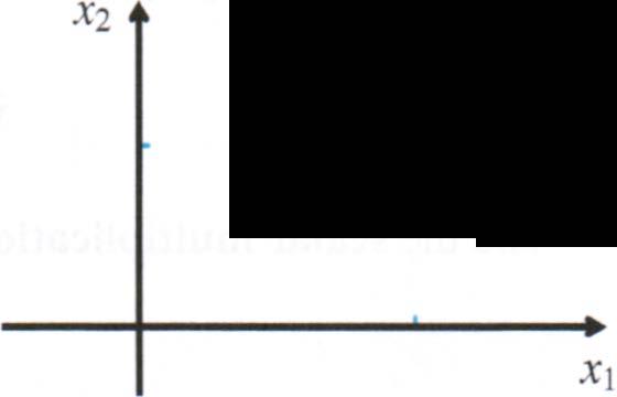
We begin by considering the two-dimensional plane in Cartesian coordinates. Choose an origin 0 and two mutually perpendicular axes, called the x1 -axis and the xraxis, as shown in Figure 1.1.1. Then a point Pin the plane is identified by the 2-tuple (p1, p2), calledcoordinates of P, where Pt is the distance from Pto the X2-axis, with p1 positive if Pisto the rightofthisaxis andnegative if Pisto the left. Similarly, p2 isthe distance from Pto the x1 -axis, with p2 positive if Pis above thisaxisandnegative if Pis below. You have already learned how to plot graphs of equations in this plane.
p2)
Figure 1.1.1 Coordinates in the plane .
For applications in many areas of mathematics, and in many subjects such as physics and economics, it is useful to view points more abstractly. In particular, we will view them as vectors and provide rules for adding them and multiplying them by constants.
Definition
Definition
Addition and Scalar Multiplication in :12
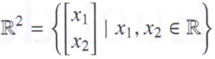
JR2 is the set of all vectors of the form [:� l where xi and x2 are real numbers called the components of the vector. Mathematically, we write
Remark
We shall use the notation 1 = [:� ] to denote vectors in JR2.
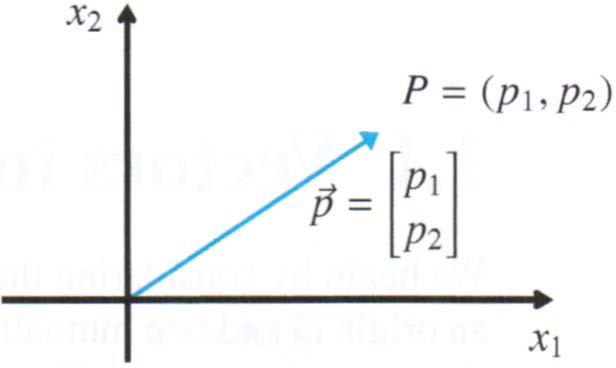
Although we are viewing the elements of JR2 as vectors, we can still interpret these geometrically as points. That is, the vector jJ = [��] can be interpreted as the point P(pi, p2). Graphically, this is often represented by drawing an arrow from (0, 0) to (pi, p2), as shown in Figure 1.1.2. Note, however, that the points between (0, 0) and (pi, p2) should not be thought of as points "on the vector." The representation of a vector as an arrow is particularly common in physics; force and acceleration are vector quantities that can conveniently be represented by an arrow of suitable magnitude and direction.
0 = (0, 0)
Figure 1.1.2 Graphical representation of a vector.
If 1 = [:� l y = [�� l and t E JR, then we define addition of vectors by X + y = [Xi]+ [y'] = [Xi + Yl] X2 Y2 X2 + Y2
and the scalar multiplication of a vector by a factor oft, called a scalar, is defined by tx = t [xi]= [txi] Xz tx2
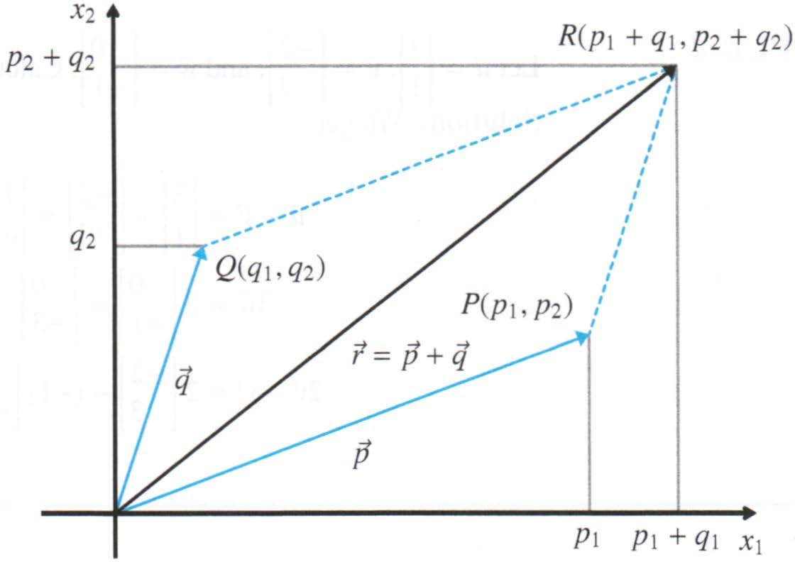
The addition of two vectors is illustrated in Figure 1.1.3: construct a parallelogram with vectors 1 and y as adjacent sides; then 1 + y is the vector corresponding to the vertex of the parallelogram opposite to the origin. Observe that the components really are added according to the definition. This is often called the "parallelogram rule for addition."
1.1.3 Addition of vectors jJ and if.
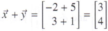
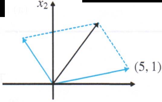
EXAMPLE I
Let x = [-�] and y = [n Then (-2, 3) 0 (3, 4) X1
Similarly, scalar multiplication is illustrated in Figure 1.1.4. Observe that multiplication by a negative scalar reverses the direction of the vector. It is important to note that x - y is to be interpreted as x + (-1)y.
1.1.4 Scalar multiplication of the vector J. X1
Figure
(1.S)J (-l)J
Figure
EXAMPLE2
Let a= [n v = [ -�].and w= [-�l
Calculate a+ v, 3w, and 2V- w.
Solution: We get
a+v= [ i ] + [- �]= [!]
3w=3 [ - �] = [ - �]
2v -w= 2 [-�] +<-1) [ _ �]= [-�] + [�] = [-�]
EXERCISE 1
Let a= [ _ � l v = [� ].and w= rn
Calculate each of the following and illustrate with a sketch.
(a) a+w (b) -v (c) (a+ w) -v
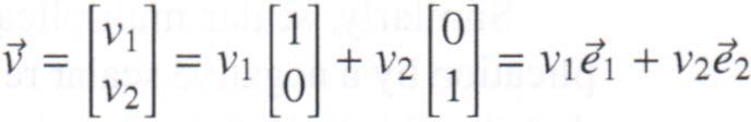
The vectors e1 = [�] and e2= [�] play a special role in our discussion of IR.2. We will call the set {e1, e2} the standard basis for IR.2. (We shall discuss the concept of a basis fmther inSection 1.2.) The basis vectors e1 and e2 are important because any vector v= [�� ] can be written as a sum of scalar multiples of e1 and e2 in exactly one way:
Remark
In physics and engineering, it is common to use the notation i instead. [�] and j = [�]
We will use the phrase linear combination to mean "sum of scalar multiples." So, we have shown above that any vector x E IR.2 can be written as a unique linear combination of the standard basis vectors.
One other vector in IR.2 deserves special mention: the zero vector, 0= [�].Some important properties of the zero vector, which are easy to verify, are that for any xEJR.2,
(1) 0+x = x
(2) x + c-1)x = o
(3) Ox=0
The Vector Equation of a Line in JR.2
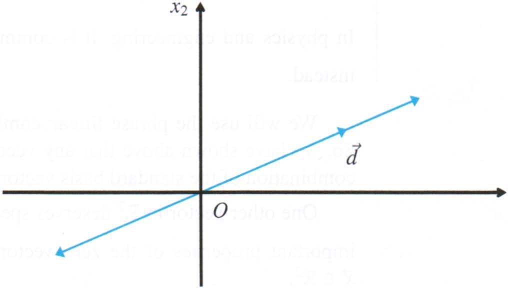
In Figure 1.1.4, it is apparent that the set of all multiples of a vector Jcreates a line through the origin. We make this our definition of a line in JR.2: a line through the origin in JR.2 is a set of the form {tJitEJR.}
Often we do not use formal set notation but simply write the vector equation of the line:
X = rJ, tEJR.
The vector Jis called the direction vector of the line. Similarly, we define the line through ff with direction vector Jto be the set
{ff+ tJi tEJR.}
which has the vector equation
X = ff+ rJ. tEJR.
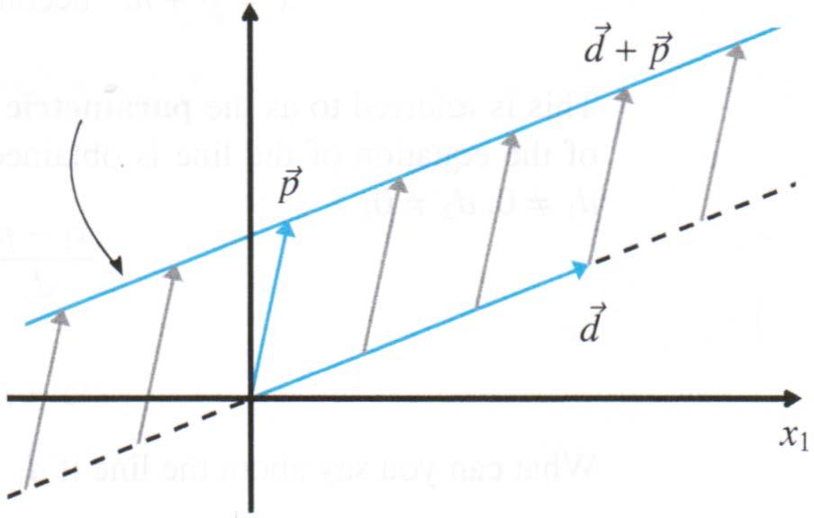
This line is parallel to the line with equation x = rJ. tEJR. because of the parallelogram rule for addition. As shown in Figure 1.1.5, each point on the line through ff can be obtained from a corresponding point on the line x = rJ by adding the vector ff. We say that the line has been translated by ff. More generally, two lines are parallel if the direction vector of one line is a non-zero multiple of the direction vector of the other line.
X2 line x = rJ+ ff
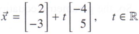
1.1.5 The line with vector equation x = td + p. A vector equation of the line through the point P(2, -3) with direction vector [ -� ] is
Figure
EXAMPLE4
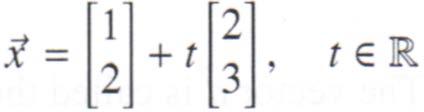
Write the vector equation of a line through P(l, 2) parallel to the line with vector equation
x= t [ � ] , tEIR
Solution: Since they are parallel, we can choose the same direction vector. Hence, the vector equation of the line is
EXERCISE 2
Write the vector equation of a line through P(O, 0) parallel to the line with vector equation
Sometimes the components of a vector equation are written separately:
J
{ X1 = Pl + td1 x = jJ + t becomes X2 = P2 + td2, t EIR
This is referred to as the parametric equation of the line. The familiar scalar form of the equation of the line is obtained by eliminating the parameter t. Provided that di* 0, d1* 0, or
X1-Pl X2-P2 ----r---di d1
d1
x2 = P2 + di(xi-Pi)
What can you say about the line if d1 = 0 or d2 = O?
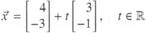
EXAMPLES
Write the vector, parametric, and scalar equations of the line passing through the point P(3, 4) with direction vector r-�].
Solution: The vector equation is x = [!] + t r-�l t ER
. . . { XI = 3 - St
So, the parametnc equat10n 1s X2 = 4 + t, tER
The scalar equation is x2 = 4 - !Cx1 - 3).
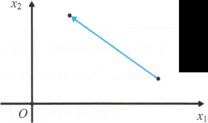
Directed Line Segments For dealing with certain geometrical problems, it is useful to introduce directed line segments. We denote the directed line segment from point P to point Q by PQ. We think of it as an "arrow" starting at P and pointing towards Q. We shall identify directed line segments from the origin 0 with the corresponding vectors; we write OP = fJ, OQ=if, and so on. A directed line segment that starts at the origin is called the position vector of the point.
For many problems, we are interested only in the direction and length of the directed line segment; we are not interested in the point where it is located. For example, in Figure 1.1.3, we may wish to treat the line segment QR as if it were the same as OP. Taking our cue from this example, for arbitrary points P, Q, R in JR.2, we define QR to be equivalent to OP if r -if=fJ. In this case, we have used one directed line segment OP starting from the origin in our definition.
More generally, for arbitrary points Q, R, S, and T in JR.2, we define QR to be equivalent to ST if they are both equivalent to the same OP for some P. That is, if r-if = fJ and t- s=fJ for the same fJ
We can abbreviate this by simply requiring that r-if=i'-s
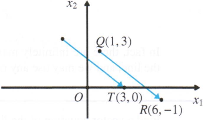
For points Q(l, 3), R(6,-l), S(-2,4), and T(3,0), we have that QR is equivalent to ST because -r - if= [ �] -[ �] = [ -�] = [�] -[ -!] = r- s
S(-2,4)
Figure 1.1.6 A directed line segment from P to Q.
EXAMPLE 7
EXERCISE 3
In some problems, where it is not necessary to distinguish between equivalent directed line segments, we "identify" them (that is, we treat them as the same object) and write PQ= RS. Indeed, we identify them with the corresponding line segment starting at the origin, so in Example 6 we write QR =ST = [-�l
Remark
Writing QR = ST is a bit sloppy-an abuse of notation-because QR is not really the same object as ST. However, introducing the precise language of "equivalence classes" and more careful notation with directed line segments is not helpful at this stage. By introducing directed line segments, we are encouraged to think about vectors that are located at arbitrary points in space. This is helpful in solving some geometrical problems, as we shall see below.
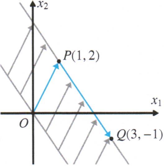
Find a vector equation of the line through P(l, 2) and Q(3, -1).
Solution: The direction of the line is
Hence, a vector equation of the line with direction PQ that passes through P( 1, 2) is x=p+tPQ=[;]+t[_i]•tE�
Observe in the example above that we would have the same line if we started at the second point and "moved" toward the first point--0r even if we took a direction vector in the opposite direction. Thus, the same line is described by the vector equations
x=[_iJ+r[-�J.rE�
x=[iJ+s[_iJ·sE� x=[;]+t[-�],tE�
In fact, there are infinitely many descriptions of a line: we may choose any point on the line, and we may use any non-zero multiple of the direction vector.
Find a vector equation of the line through P(l, 1) and Q(-2, 2).
Vectors and Lines in R3
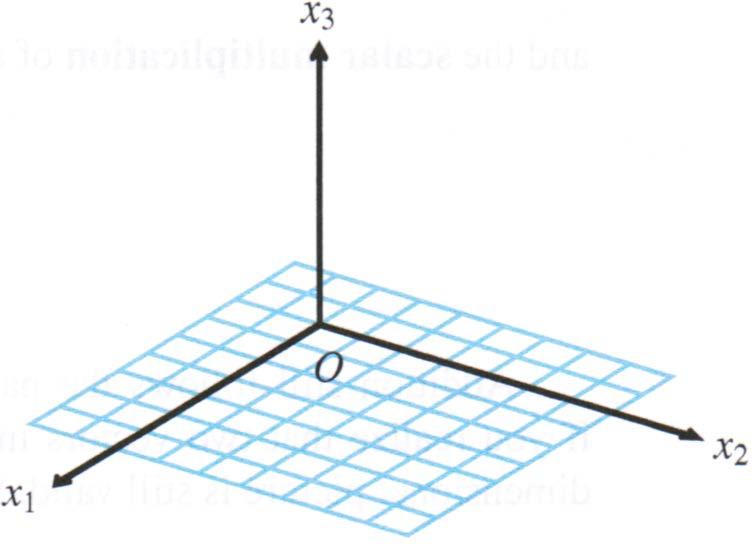
Everything we have done so far works perfectly well in three dimensions. We choose an origin 0 and three mutually perpendicular axes, as shown in Figure 1.1.7. The x1-axis is usually pictured coming out of the page (or blackboard), the x2-axis to the right, and thex3-axis towards the top of the picture.
1.1.7 The positive coordinate axes in IR.3.
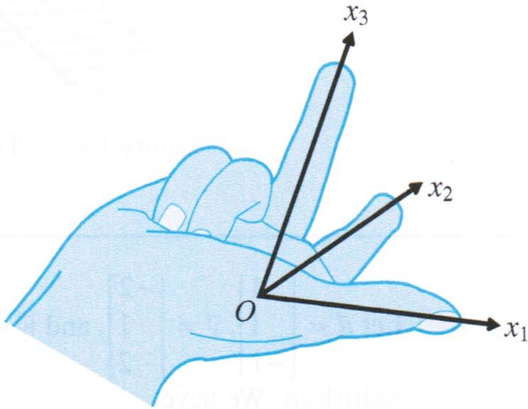
It should be noted that we are adopting the convention that the coordinate axes form a right-handed system. One way to visualize a right-handed system is to spread out the thumb, index finger, and middle finger of your right hand. The thumb is the x1-axis, the index finger is the x2-axis, and the middle finger is the x3-axis. See Figure 1.1.8.
1.1.8 Identifying a right-handed system.
We now define JR.3 to be the three-dimensional analog of JR.2.
R3 is the set of all vectors of the form
Mathematically, we write
· wherex1,x,, andx3 are ceal numbers.
Figure
Figure
Definition
Addition and Scalar Multiplication in J.3
EXAMPLES
If 1 = [:n jl = �n and t E II., then we define addition of vectors by [Xt l l [Xt + Yt l x + y = X2 + Y2 = X2 + Y2 X3 3 X3 + Y3 and the scalarmultiplication of a vector by a factor oft by [Xl l [tX1 l tx = t x2 = tx2 X3 tX3
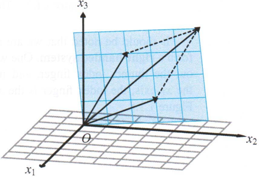
Addition still follows the parallelogram rule. It may help you to visualize this if you realize that two vectors in JR.3 must lie within a plane in JR.3 so that the twodimensional picture is still valid. See Figure 1.1.9.
Figure 1.1.9
Two-dimensional parallelogram rule in IR.3.
Let u = [_i]. jl = l-n and w = [H crucula� jl +U, -W, and -V + 2W - u.
Solution: We have V+U = nHJ = ni -w = -[�] {�] -V + 2W-" = - l-11+2 l�l-lJ = l=rl + m + l = :1 = r-�l
Section 1.1 Vectors in JR.2 and JR.3
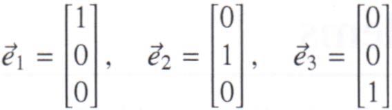
It is useful to introduce the standard basis for JR.3 just as we did for JR.2. Define
Then any vector V = [�:] can be written as the linear combination
Remark
In physics and engineering,it is common to use the notation i = e1, j = e1, and k = e3 instead.
The zero vector 0 = [�] in R3 has the same properties as the zero vector in l!.2.
Directed line segments are the same in three-dimensional space as in the twodimensionalcase.
A line through the point P in JR.3 (corresponding to a vector {J) with direction vector J f. 0 can be described by a vector equation:
X = p + tJ, t E JR
It is important to realize that a line in JR.3 cannot be described by a single scalar linear equation, as in JR.2. We shall see in Section 1.3 that such an equation describes a plane in JR.3.
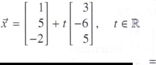
Find a vector equation of the line that passes through the points P(l, 5, -2) and Q(4,-1,3).
Solution: A direction vector is J = if - p = [-H Hence a vector equation of the line is
Note that the corresponding parametric equations are x1 X3 = -2 +St. 1 + 3t, x2 = 5 - 6t, and
Find a vector equation of the line that passes through the points P(l, 2,2) and Q(l,-2,3).
PROBLEMS 1.1
Practice Problems
Al Computeeachofthefollowinglinearcombinations andillustratewithasketch.
(a)[�]+[�]
(c)3 [- �]
A2 Compute each of the following linear combinations.
(a)[-�]+[-�]
(c)-2 [_;J
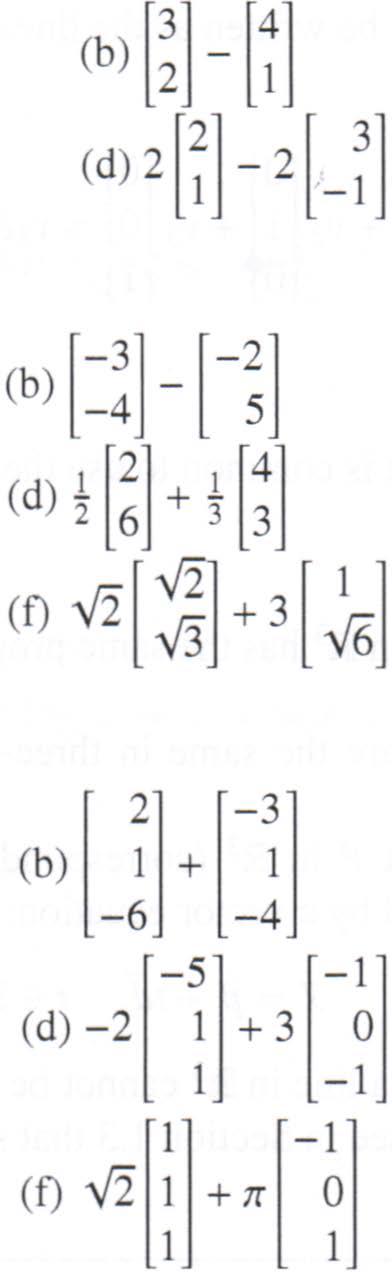
2 [3] [1/4) (e) 3 1 - 2 1/3
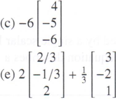
A3 Compute each of the following linear combinations.
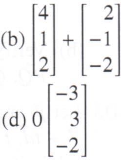
(a) [!]-[J
A4 Ut V = Ul and W= Hl Detenillne
(a) 2v- 3w
Cb) -3Cv +2w)+5v
(c) a suchthat w- 2a = 3v (d) a suchthat a- 3v = 2a
AS Ut V = m and W = r =n Detennine
(a) �v +!w
Cb) 2c v + w)- c2v- 3w)
(c) a suchthat w-a = 2V (d) a suchthat!a + �v= w
A6 Consider the points P(2,3,1), Q(3,1,-2), R(l,4,0), S(-5,1,5). Determine PQ, PR, PS,QR, and SR, andverifythat PQ+QR= PR= PS+ SR.
AJO (a) A setofpointsin IR.11 is collinear ifallthepoints lieonthesameline.Byconsideringdirected linesegments,giveageneralmethodfordeterminingwhetheragivensetofthreepointsis collinear.
(b) Determinewhetherthepoints P(l,2),QC4,1), and R(-5,4) are collinear. Show how you decide.
(c)Determine whether the points S(1,0,1), T(3,-2,3), and U(-3,4,-1) are collinear. Showhowyoudecide.
Homework Problems
B 1 Compute each of the following linear combinations and illustrate with a sketch.
(a) [-�] +r-�]
(c) -3 [-�]
(b) [-�]- [�]
(d) -3 [�]- [;]
B2 Compute each of the following linear combinations.
(a)[�]+ [=�]
(c) 2 [=�J
(b) [�]- [�]
(dH [1�]- ?a[�]
(e) �[ � + Y3 [- �12] - [ �]
B3 Compute each of the following linear combinations.
<{�]-[-�]
(c) 4 [=�l
(e) f;�l +l Hl
(f) (1 +�) 10 _ i [-�1 �-i J 2
B4 Ut V {�l and W {n Detecm;ne
(a) 2v- 3w
(b) -2(v- w) - 3w
(c) i1 such that w - 2i1 = 3v
(d) i1 such that 2i1 + 3w= v
BS Ut V = [ -�] and W= [-H Deterrlline
(a) 3v- 2w
(b) -iv+�w
(c) i1 such that v+i1= v
(d) i1 such that 2i1 -w= 2v
B6 (a) Consider the points P(l,4,1), Q(4,3,-1), R(-1,4,2), and S(8,6,-5). Determine PQ, PR,PS, QR,and SR,and verify that PQ+QR= PR= PS +SR.
(b) Consider the points P(3,-2,1), Q(2,7, -3), R(3,1,5), and S(-2,4,-1). Determine PQ, -t -+-+ PK, PS, QR, and SR,and verify that PQ+QR= PR= PS +SR.
B7 Write a vector equation of the line passing through the given points with the given direction vector.
(a) P(-3,4),J= [-�]
(b) P(O, 0). J= m
(c) P(2,3,-1), J= [-�]
(d) P(3,1,2),J=[-�]
BS Write a vector equation for the line that passes through the given points.
(a) P(3,1), Q(l,2)
(b) P(l,-2,1), Q(O,0,0)
(c) P(2,-6,3), Q(-1,5,2)
(d) P(l,-1,i), Q(i,t. 1)
B9 For each of the following lines in JR2, determine a vector equation and parametric equations.
(a) x2= -2x1 + 3
(b) Xi + 2X2= 3
BlO (You will need the solution from Problem AlO (a) to answer this.)
(a) Determine whether the points P(2,1,1), Q(l,2, 3), and R(4,-1,-3) are collinear. Show how you decide.
(b) Determine whether the points S(1,1,0), T(6,2,1),and U(-4, 0,-1) are collinear. Show how you decide.
Computer Problems
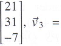
Cl Let V, = [=�u V2 � [-361 -�: , and v, = [=m
Use computer software to evaluate each of the following.
(a) 171!1 + sv2 - 3v3 + 42v4
(b) -1440i11 - 2341i12 - 919i13 + 6691/4
Conceptual Problems
Dl Let i1 = [ �] and w = [ _ �].
(a) Find real numbers t1 and t2 such that t1i1+t2w = [ _ � � l Illustrate with a sketch.
(b) Find real numbers t1 and t2 such that t1 v+t2w = [��] for any X1,X2 E R
(c) Use your result in part (b) to find real numbers t1 and t2 such that t1V1 + t2i12 = [ :2).
D2 Let P, Q, and R be points in JR.2 corresponding to vectors fl, q, and rrespectively.
(a) Explain in terms of directed line segments why PQ+QR+RP = o
(b) Verify the equation of part (a) by expressing PQ, QR, and RP in terms of jJ, q, and r.
D3 Let fl and J t= 0 be vectors in JR.2. Prove that x = fl + tJ, t E JR, is a line in JR.2 passing through the origin if and only if fl is a scalar multiple of J
D4 Let x and y be vectors in JR.3 and t E JR be a scalar. Prove that t(x +y) = tx+ t)!
1.2 Vectors in IRn
We now extend the ideas from the previous section to n-dimensional Euclidean space JR.11•
Students sometimes do not see the point in discussing n-dimensional space becauseit does not seemtocorrespondtoanyphysicalrealisticgeometry. But, in a number of instances, more than three dimensions are important. For example, to discuss themotion of aparticle, an engineer needs to specifyitsposition (3 variables) andits velocity (3 morevariables); theengineer thereforehas 6 variables. Ascientist working in string theory works with 11 dimensionalspace-time variables. An economist seeking to model the Canadian economy uses many variables: one standard model has more than 1500 variables. Of course, calculations in such huge models are carried out by computer. Even so, understanding the ideas ofgeometry andlinear algebra is necessary to decide which calculations are required andwhat the results mean.
Definition
Definition
Addition and Scalar Multiplication in :i"
Addition and Scalar Multiplication of Vectors in JRn
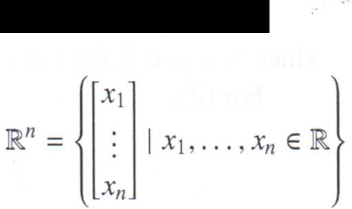
JR.11 is the set of all vectors of the form : , where x; E R Mathematically, Xn If 1 = Xi , y = 11 , and t E JR., then we define addition of vectors by Xn
Theorem 1
l [X1 +Yl x+.Y= : + : = : Xn n Xn +Yn and the scalarmultiplication of a vector by a factor oft by tx= t 1�1] = t�1] Xn tX11
J'.or all w, x, y E JR.11 ands, t E JR. we have
(1) x+y E JR.11 (closed under addition) (2) x+y= y+ 1 (addition is commutative) (3) c1+y)+ w = 1+CY+ w) (addition is associative) •
(4) There exists a vector 0 E JR.11 such that z+0 = z for all E JR.ll (zero vector) (5) For each 1 E JR.ll there exists a vector -1 E JR.11 such that 1 + (-1) = 0 (additive inverses)
(6) t1 E JR.11 (closed under scalar multiplication) (7) s(t1) = (st)1 (scalar multiplication is associative) (8) (s + t)x= s1+tx (a distributive law) (9) t(1 +y)= t1+tY (another distributive law) (10) lx = 1 (scalar multiplicative identity)
Proof: We will prove properties (1) and (2) from Theorem 1 and leave the other proofs to the reader.