Table of Contents
Preface
About the Author
Chapter 1. Introduction
1.1 Introduction
1.2 Instrumentation
1.3 Process Models and Dynamic Behavior
1.4 Redundancy and Operability
1.5 Industrial IoT and Smart Manufacturing
1.6 Control Textbooks
1.7 A Look Ahead
1.8 Summary References
Chapter 2. Fundamental Models
2.1 Background
2.2 Balance Equations
2.3 Material Balances
2.4 Constitutive Relationships
2.5 Material and Energy Balances
2.6 Form of Dynamic Models
2.7 Linear Models and Deviation Variables
2.8 Summary
Chapter 3. Dynamic Behavior
3.1 Background
3.2 Linear State-Space Models
3.3 Laplace Transforms
3.4 Transfer Functions
3.5 First-Order Behavior
3.6 Integrating Behavior Purely Integrating Systems
3.7 Second-Order Behavior
3.8 Summary References
Chapter 4. Dynamic Behavior: Complex Systems
4.1 Introduction
4.2 Poles and Zeros
4.3 Lead-Lag Behavior
4.4 Processes with Deadtime
4.5 Padé Approximation for Deadtime
4.6 Converting State-Space Models to Transfer Functions
4.7 Converting Transfer Functions to State-Space Models
4.8 Matlab and Simulink
4.9 Summary
Chapter 5. Empirical and Discrete-Time Models
5.1 Introduction
5.2 First-Order + Deadtime
5.3 Integrator + Deadtime
5.4 Other Continuous Models
5.5 Discrete-Time Autoregressive Models
5.6 Parameter Estimation
5.7 Discrete Step and Impulse Response Models
5.8 Converting Continuous Models to Discrete
5.9 Digital Filtering
5.10 Summary References
Chapter 6. Introduction to Feedback Control
Chapter 7. Model-Based Control
7.1 Introduction
7.2 Direct Synthesis
7.3 Internal Model Control
7.4 IMC-Based PID
7.5 IMC-Based PID Design for Processes with a Time Delay
7.6 IMC-Based PID Controller Design for Unstable Processes
7.7 Summary References
Chapter 8. PID Controller Tuning
8.1 Introduction
8.2 Closed-Loop Oscillation-Based Tuning
8.3 Tuning Rules for First-Order + Deadtime Processes
8.4 Digital Control
8.5 Stability of Digital Control Systems
8.6 Performance of Digital Control Systems
8.7 Summary References
Chapter 9. Frequency-Response Analysis
9.1 Motivation
9.2 Bode and Nyquist Plots
9.3 Effect of Process Parameters on Bode and Nyquist Plots
9.4 Closed-Loop Stability
9.5 Bode and Nyquist Stability
9.6 Robustness
9.7 Matlab Control Toolbox: Bode and Nyquist Functions
9.8 Summary
Chapter 10. Cascade and Feedforward Control
10.1 Background
10.2 Introduction to Cascade Control
10.3 Cascade-Control Analysis
10.4 Cascade-Control Design
10.5 Feedforward Control
10.6 Feedforward Controller Design
10.7 Summary of Feedforward Control
10.8 Combined Feedforward and Cascade
10.9 Summary
Chapter 11. PID Enhancements
Chapter 12. Ratio, Selective, and Split-Range Control
12.1 Motivation
12.2 Ratio Control
12.3 Selective and Override Control
12.4 Split-Range Control
12.5 Simulink Functions
12.6 Summary
Chapter 13. Control-Loop Interaction
13.1 Introduction
13.2 Motivation
13.3 The General Pairing Problem
13.4 The Relative Gain Array
13.5 Properties and Application of the RGA Sum of Rows and Columns
13.6 Return to the Motivating Example
13.7 RGA and Sensitivity
13.8 Using the RGA to Determine Variable Pairings
13.9 Matlab RGA Function File
13.10 Summary References
Appendix 13.1: Derivation of the Relative Gain for an nInput–n-Output System
Chapter 14. Multivariable Control
Chapter 15. Plantwide Control
Chapter 16. Model Predictive Control
Chapter 17. Summary
Module 1. Introduction to MATLAB
Module 2. Introduction to SIMULINK
Module 3. Ordinary Differential Equations
Module 4. MATLAB LTI Models
Module 5. Isothermal Chemical Reactor
Module 6. First-Order + Time-Delay Processes
Module 7. Biochemical Reactors
Module 8. CSTR
Module 9. Steam Drum Level
Module 10. Surge Vessel Level Control
Module 11. Batch Reactor
Module 12. Biomedical Systems
Module 13. Distillation Control
Module 14. Case Study Problems
Module 15. Plug Flow Reactor
Module 16. Digital Control
Preface
This content is currently in development.
Chapter 1. Introduction
The goal of this chapter is to provide a motivation for and an introduction to process control and instrumentation. After studying this chapter, the reader, given a process, should be able to
• Determine possible control objectives, input variables (manipulated and disturbance) and output variables (measured and unmeasured), and constraints (hard or soft), as well as classify the process as continuous, batch, or semicontinuous.
• Assess the importance of process control from safety, environmental, and economic points of view.
• Sketch a process instrumentation and control diagram.
• Draw a simplified control block diagram.
• Understand the basic ideas of feedback and feedforward control.
• Understand basic sensors (measurement devices) and actuators (manipulated inputs).
• Begin to develop intuition about characteristic timescales of dynamic behavior.
• Describe simple control loops associated with physiological systems. The major sections of this chapter are as follows:
1.1 Introduction
1.2 Instrumentation
1.3 Process Models and Dynamic Behavior
1.4 Redundancy and Operability
1.5 Industrial IoT and Smart Manufacturing
1.6 Control Textbooks and Journals
1.7 A Look Ahead
1.8 Summary
1.1 Introduction
Process engineers are often responsible for the operation of chemical processes. As these processes become larger in scale and/or more complex, the role of process automation becomes increasingly important. The primary objective of this textbook is to teach process engineers how to design and tune controllers for the automated operation of chemical processes.
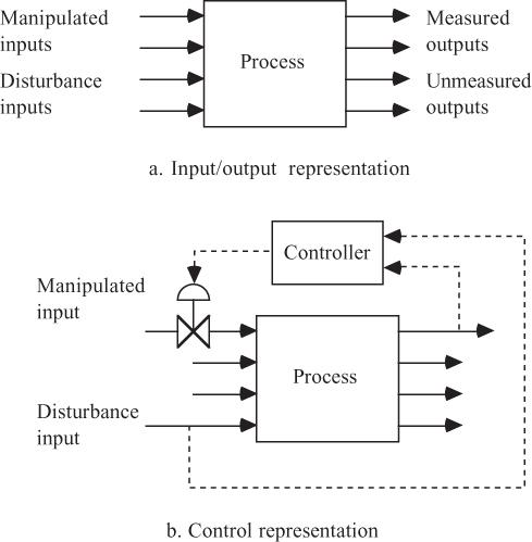
A conceptual process block diagram for a chemical process is shown in Figure 1–1. Notice that inputsare classified as either manipulated or disturbance, and the outputsare classified as measured or unmeasured in Figure 1–1a. To automate the operation of a process, it is important to use measurements of process outputs or disturbance inputs to make decisions about the proper values of manipulated inputs. This is the purpose of the controller shown in Figure 1–1b; the measurement and control signals are shown as dashed lines. These initial concepts probably seem very vague or abstract at this point. Do not worry, because we present a number of examples in this chapter to clarify these ideas.
The development of a control strategy consists of formulating or identifying the following:
1. Control objective(s)
2. Input variables
3. Output variables
4. Constraints
5. Operating characteristics
6. Safety, environmental, and economic considerations
7. Control structure
We discuss in more detail the steps in formulating a control problem:
1. The first step of developing a control strategy is to formulate the control objective(s). A chemical-process operating unit often consists of several unit operations. The control of an operating unit is generally reduced to considering the control of each unit operation separately. Even so, each unit operation may have multiple, sometimes conflicting objectives, so the development of control objectives is not a trivial problem.
Figure 1–1 Conceptual process input/output block diagram
2. Input variables can be classified as manipulatedor disturbance variables. A manipulated input is one that can be adjusted by the control system (or process operator). A disturbance input is a variable that affects the process outputs but that cannot be adjusted by the control system. Inputs may change continuouslyor at discreteintervals of time.
3. Output variables can be classified as measuredor unmeasured variables. Measurements may be made continuouslyor at discrete intervals of time.
4. All processes have certain operating constraints,which are classified as hard or soft. An example of a hard constraint is a minimum or maximum flow rate—a valve operates between the extremes of fully closed or fully open. An example of a soft constraint is a product composition—it may be desirable to specify a composition between certain values to sell a product, but it is possible to violate this specification without posing a safety or environmental hazard.
5. Operating characteristics are usually classified as continuous, batch,or semi-continuous(semibatch).Continuous processes operate for long periods of time under relatively constant operating conditions before being shut down for cleaning, catalyst regeneration, and so forth. For example, some processes in the oilrefining industry operate for 18 months between shutdowns. Batch processes are dynamic in nature—that is, they generally operate for a short period of time, and the operating conditions may vary quite a bit during that time. Example batch processes include beer or wine fermentation, as well as many specialty chemical processes. For a batch reactor, an initial charge is made to the reactor, and conditions (temperature, pressure) are varied to produce a desired product at the end of the batch time. A typical semibatch process may have an initial charge to the reactor, but feed components may be added to the reactor during the course of the batch run.
Another important consideration is the dominant timescale of a process. For continuous processes, this is very often related to the residence time of the vessel. For example, a vessel with a liquid volume of 100 liters and a flow rate of 10 liters/minute would have a residence time of 10 minutes; that is, on the average, an element of fluid is retained in the vessel for 10 minutes.
6. Safety, environmental, and economic considerations are all very important. In a sense, economics is the ultimate driving force—an
unsafe or environmentally hazardous process will ultimately cost more to operate because of fines paid, insurance costs, and so forth. In many industries (petroleum refining, for example), it is important to minimize energy costs while producing products that meet certain specifications. Better process automation and control allows processes to operate closer to optimum conditions and to produce products where variability specifications are satisfied.
The concept of failsafe is always important in the selection of instrumentation. For example, a control valve needs an energy source to move the valve stem and change the flow; most often, this is a pneumatic signal (usually 3–15 psig). If the signal is lost, then the valve stem will go to the 3-psig limit. If the valve is air-toopen,then the loss of instrument air will cause the valve to close; this is known as a fail-closedvalve. If, on the other hand, a valve is air-to-close,when instrument air is lost, the valve will go to its fully open state; this is known as a fail-openvalve. These concepts are illustrated in Figure 1–2.
7. The two standard control types are feedforwardand feedback. A feedforward controller measures the disturbance variable and sends this value to a controller, which adjusts the manipulated variable. A feedback control system measures the output variable, compares that value to the desired output value, and uses this information to adjust the manipulated variable. For the first part of this book, we emphasize feedback control of single-input (manipulated) and single-output (measured) systems. Determining the feedback control structure for these systems consists of deciding which manipulated variable will be adjusted to control which measured variable. The desired value of the measured process output is called the setpoint.
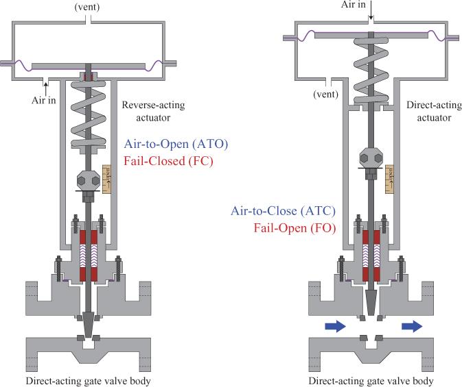
Figure 1–2 Fail-closed and fail-open valves. The fail-closed valve (left) has instrument air entering below the actuator, whereas the fail-open valve (right) has instrument air engineering above the actuator. In each case, the loss of instrument air will cause the valve to move in the direction forced by the spring attached to the actuator. Source:GlobalSpec, s.v. How can we change the action of a control valve? Response by tonykuphaldt, September 2011, http://cr4.globalspec.com/thread/75751/How-Can-We-Change-theAction-of-a-Control-Valve.
A particularly important concept used in control system design is process gain. The process gain is the sensitivity of a process output to a change in the process input. If an increase in a process input leads to
an increase in the process output, it is known as a positive gain. Conversely, if an increase in the process input leads to a decrease in the process output, it is known as a negative gain. The magnitude of the process gain is also important. For example, a change in power (input) of 0.5 kW to a laboratory-scale heater may lead to a fluid temperature (output) change of 10°C; this change is a process gain (change in output/change in input) of 20°C/kW. The same input power change of 0.5 kW to a larger-scale heater may yield an output change of only 0.5°C, corresponding to a process gain of 1°C/kW.
Once the control structure is determined, it is important to decide on the control algorithm. The control algorithm uses measured output variable values (along with desired output values) to change the manipulated input variable. A control algorithm has a number of control parameters,which must be tuned (adjusted) to have acceptable performance. Often, the tuning is done on a simulation model before implementing the control strategy on the actual process. Also, many advanced strategies use model-basedcontrol, that is, controllers with a built-in model of the process.
This approach is best illustrated by way of example. Because many important concepts, such as control instrumentation diagrams and control block diagrams, are introduced in the next examples, it is important that you study them thoroughly.
Example 1.1: Surge Tank
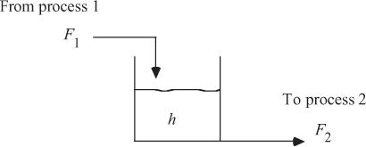
Surge tanks are often used as intermediate storage for fluid streams being transferred between process units. Consider the process flow diagram shown in Figure 1–3, where a fluid stream from process 1 is fed to the surge tank; the effluent from the surge tank is sent to process 2.
There are obvious constraints on the height in this tank. If the tank overflows, it may create safety and environmental hazards, which may also have economic significance. Let us analyze this system using a step-by-step procedure.
1. Controlobjective:The control objective is to maintain the height within certain bounds. If it is too high, it will overflow, and if it is too low, problems with the flow to process 2 may occur. Usually, a specific desired height will be selected. This desired height is known as the setpoint.
2. Inputvariables:The input variables are the flow from process 1 and the flow to process 2. Noticethatanoutletflowrateis consideredaninputtothissystem.The question is, which input is manipulated and which is a disturbance? That depends. We discuss this problem further in a moment.
3. Outputvariables:The most important output variable is the liquid level. We assume that it is measured.
1–3 Tank level problem
4. Constraints:A number of constraints exist in this problem. There is a maximum liquid level; if it is exceeded, the tank will overflow. There are minimum and maximum flow rates through the inlet and outlet valves.
5. Operatingcharacteristics:We assume that this is a continuous process, that is, that there is a continuous flow in and out of the tank. It would be a semicontinuous process if, for example, there was an inlet flow with no outlet flow (if the tank was simply being filled).
6. Safety,environmental,andeconomicconsiderations:These aspects depend somewhat on the fluid characteristics. If it is a hazardous chemical, then there is a tremendous incentive from safety and environmental considerations to not allow the tank to
Figure
overflow. Indeed, this is also an economic consideration, because injuries to employees or environmental cleanup costs money. Even if the substance is water, it has likely been treated by an upstream process unit, so losing water owing to overflow will incur an economic penalty.
Safety considerations play an important role in the specification of control valves (fail-open or fail-closed). For this particular problem, the control-valve specification will depend on which input is manipulated. This is discussed in detail shortly.
7. Controlstructure:There are numerous possibilities for control of this system. We discuss first the feedback strategies, then the feedforward strategies.
Feedback Control
The measured variable for a feedback control strategy is the tank height. Which input variable is manipulated depends on what is happening in process 1 and process 2. Let us consider two different scenarios. In scenario 1, process 2 regulates the flow rate F2, leaving F1 to be manipulated by a controller. In scenario 2, process 1 regulates the flow rate F1, leaving F2 to be manipulated by a controller. Here we further discuss scenario 2; scenario 1 is used as a student exercise (exercise 5).
Scenario2Process 1 regulates flow rate F1. This could happen, for example, if process 1 is producing a chemical compound that must be processed by process 2. Perhaps process 1 is set to produce F1 at a certain rate. F1 is then considered “wild” (a disturbance) by the tank process. In this case, we would adjust F2 to maintain the tank height. Notice that the control valve should be specified as fail-open or air-toclose so that the tank will not overflow on loss of instrument air or other valve failure.
The control and instrumentation diagram for a feedback control strategy for this scenario is shown in Figure 1–4a. Notice that the level transmitter (LT) sends the measured height of liquid in the tank (hm) to
the level controller (LC). The LC compares the measured level with the desired level (hsp, the height setpoint) and sends a pressure signal (Pv) to the valve. This valve op pressure moves the valve stem up and down, changing the flow rate through the valve (F2). If the controller is designed properly, the flow rate changes to bring the tank height close to the desired setpoint. In this process and instrumentation diagram, we use dashed lines to indicate signals between different pieces of instrumentation.
Figure 1–4 Instrumentation and control block diagrams for the tank level feedback control problem. The outlet flow rate (F2) is manipulated, the inlet flow rate (F1) is a disturbance, and the tank height (h) is measured and controlled.
A simplified block diagram representing this system is shown in Figure 1–4b. Each signal and device (or process) is shown on the block diagram. We use a slightly different form for block diagrams when we
use transfer function notation for control system analysis in Chapter 5, “Empirical and Discrete-Time Models.” Note that each block represents a dynamic element. We expect that the valve and LT dynamics will be much faster than the process dynamics. We also see clearly from the block diagram why this is known as a feedbackcontrol “loop.” The controller “decides” on the valve position, which affects the outlet flow rate (the manipulated input), which affects the level; the inlet flow rate (the disturbance input) also affects the level. The level is measured, and that value is fed back to the controller (which compares the measured level with the desired level [setpoint]).
Feedforward Control
The previous feedback control strategy was based on measuring the output (tank height) and manipulating an input (the outlet flow rate). In this case, the manipulated variable is changed after a disturbance affects the output. The advantage of a feedforwardcontrol strategy is that a disturbance variable is measured and a manipulated variable is changed before the output is affected. Consider the preceding case where the inlet flow rate can be changed by the upstream process unit and is therefore considered a disturbance variable. If we can measure the inlet flow rate, we can manipulate the outlet flow rate to maintain a constant tank height. This feedforward control strategy is shown in Figure 1–5a, where FM is the flow measurement device and FFC is the feedforward controller. The corresponding control block diagram is shown in Figure 1–5b. F1 is a disturbance input that directly affects the tank height; the value of F1 is measured by the FM device, and the information is used by an FFC to change the manipulated input, F2.
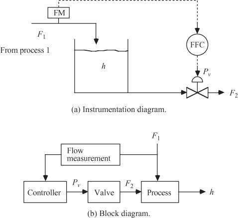
Figure 1–5 Instrumentation and control block diagrams for the tank level feedforward control problem. The inlet flow rate is measured and outlet flow rate is manipulated.
The main disadvantage to this approach is sensitivity to uncertainty. If the inlet flow rate is not perfectly measured or if the outlet flow rate cannot be manipulated perfectly, then the tank height will not be perfectly controlled. With any small disturbance or uncertainty, the tank will eventually overflow or run dry. In practice, FFC is combined with feedback control to account for uncertainty. A feedforward/feedback strategy is shown in Figure 1–6a, and the corresponding block diagram is shown in Figure 1–6b. Here, the feedforward portion allows immediate corrective action to be taken before the disturbance (inlet flow rate) actually affects the output measurement (tank height). The feedback controller adjusts the outlet flow rate to maintain the desired tank height, even with errors in the inlet flow-rate measurement.
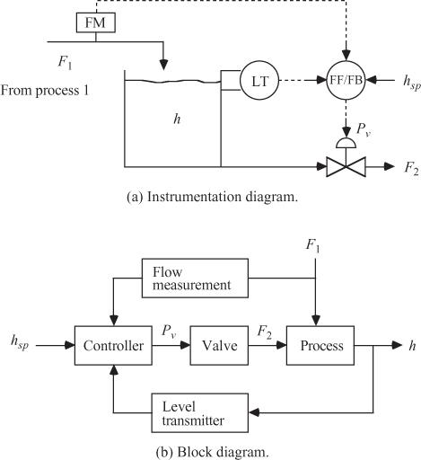
Figure 1–6 Feedforward/feedback control of tank level. The inlet flow rate is the measured disturbance, tank height is the measured output, and outlet flow rate is the manipulated input.
Discussion of Level Controller Tuning and the Dominant Timescale
Notice that we have not discussed the actual control algorithms; the details of control algorithms and tuning are delayed until Chapter 5. Conceptually, would you prefer to tune level controllers for fast or slow responses?
When tanks are used as surge vessels, it is usually desirable to tune the controllers for a slow return to the setpoint. This is particularly true for scenario 2, where the inlet flow rate is considered a disturbance
variable. The outlet flow rate is manipulated but affects another process. To avoid upsetting the downstream process, we would like to change the outlet flow rate slowly yet fast enough that the tank does not overflow or go dry.
Related to the controller tuning issue is the importance of the dominant timescale of the process. Consider the case where the maximum tank volume is 200 gallons and the steady-state operating volume is 100 gallons. If the steady-state flow rate is 100 gallons/minute, the residencetimewould be 1 minute. Assume the inlet flow rate is a disturbance and outlet flow rate is manipulated. If the feed flow rate increased to 150 gallons/minute and the outlet flow rate did not change, the tank would overflow in 2 minutes. On the other hand, if the same vessel had a steady-state flow rate of 10 gallons/minute and the inlet flow suddenly increased to 15 gallons/minute (with no change in the outlet flow), it would take 20 minutes for the tank to overflow. Clearly, controller tuning and concern about controller failure are different for these two cases.
The first example was fairly easy compared with most control-system synthesis problems in industry. Even for this simple example, we found that many issues must be considered and a number of decisions (specification of a fail-open or fail-closed valve, etc.) must be made. Often, there are many (and usually conflicting) objectives, many possible manipulated variables, and numerous possible measured variables.
It is helpful to think of common, everyday activities in the context of control to familiarize yourself with the types of control problems that can arise in practice. Examples include taking a shower (which is analyzed in the supplemental material) and driving a car. It is suggested that you work through such examples provided in problem 1 in the Student Exercises section of this chapter.
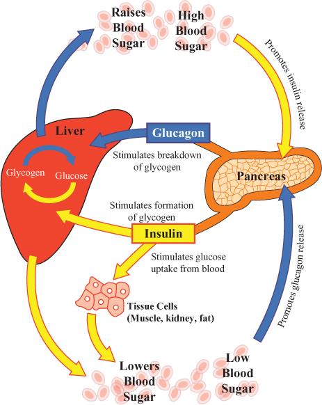
Examples of control loops abound in nature, and particularly in physiological systems. The human body regulates many variables through homeostasis; examples include temperature, blood pressure, and blood glucose—which is the topic of the next example.