Instant ebooks textbook An introduction to correspondence analysis 1st edition eric j. beh download
An Introduction to Correspondence Analysis 1st Edition Eric
J. Beh
Visit to download the full and correct content document: https://ebookmass.com/product/an-introduction-to-correspondence-analysis-1st-editio n-eric-j-beh/
More products digital (pdf, epub, mobi) instant download maybe you interests ...
An Introduction to Genetic Analysis 11th Edition, (Ebook PDF)
Table 1.1 Cross-classification ofCountry of origin of the participants and th...
Table 1.2 Temperature by Month in La Guardia airport, .
Table 1.3 Men’s shoplifting data:Item stolen versus midpoint of the perpetra...
Table 1.4 Cross-classification of 219 alligators by theirSize, primary Food o...
Table 1.5 Notation used for a contingency table.
Table 1.6 Expected cell counts, under independence, for the traditional Europ...
Table 1.7 R packages and some variants of correspondence analysis for two var...
Table 1.8 R packages and some variants of correspondence analysis for multipl...
Chapter 2
Table 2.1 The Pearson standardised residuals, , for Table 1.1.
Table 2.2 The Pearson residuals, , for the traditional European food data of ...
Table 2.3 The values from the GSVD of for Table 1.1.
Table 2.4 The values from the GSVD of for Table 1.1.
Table 2.5 The principal coordinates, , of Table 1.1.
Table 2.6 The principal coordinates, , of Table 1.1.
Table 2.7 The values of Table 1.1.
Table 2.8 Contribution and percentage contribution, of each Country catego...
Table 2.9 Contribution and percentage contribution of each Free-word categ...
Table 2.10 Features of the confidence ellipses for the Free-word categories ...
Table 2.11 Features of the confidence ellipses for the Country categories li...
Chapter 3
Table 3.1 The weighted centred column profiles, , of Table 1.1.
Table 3.2 The values from the GSVD of for Table 1.1.
Table 3.3 The values from the GSVD of for Table 1.1.
Table 3.4 The values of Table 1.1.
Table 3.5 Contribution and percentage contribution, of each Free-word cate...
Table 3.6 Contribution and percentage contribution, of each Country catego...
Table 3.7 Features of the confidence ellipses for the categories of the Free...
Table 3.8 Features of the confidence ellipses for the categories of the Coun...
Chapter 4
Table 4.1 The centred row profiles of Table 1.2.
Table 4.2 The centred column profiles of Table 1.2.
Table 4.3 The values from the BMD of for Table 1.2.
Table 4.4 The values from the BMD of for Table 1.2.
Table 4.5 The generalised correlations, , from the BMD of for Table 1.2.
Table 4.6 The values and their p-value for Table 1.2.
Chapter 5
Table 5.1 The weighted centred column profiles, , of Table 1.3.
Table 5.2 The values of Table 1.3.
Table 5.3 The values of Table 1.3.
Table 5.4 The generalised asymmetric correlations, , of Table 1.3.
Chapter 6
Table 6.1 Indicator table from the crisp coding of Table 1.4.
Table 6.2 Inertia values from the correspondence analysis of the indicator ma...
Table 6.3 Burt table of Table 1.4.
Table 6.4 Inertia values from the correspondence analysis of the Burt matrix ...
Table 6.5 Stacking ofLake and Size for the Alligator data of Table 1.4.
Table 6.6 Inertia values from the correspondence analysis of the stacked tabl...
Table 6.7 Stacking ofSize and primary Food source for the alligator data of T...
Chapter 7
Table 7.1 Partition of for Table 1.4
Table 7.2 Summary of inertia values for five combinations of , and from t...
Table 7.3 The values from the T3D of for Table 1.4
Table 7.4 The values from the T3D of for Table 1.4
Table 7.5 The values from the T3D of for Table 1.4
Table 7.6 The core array elements, from the T3D of of Table 1.4
Table 7.7 The first two sets of optimal from the T3D of of Table 1.4
Table 7.8 Column–tube principal coordinates of the column–tube interactive bi...
Table 7.9 Inner products from the symmetric multi-way correspondence analysis...
Table 7.10 Percentage of the total inertia explained by each dimension of the...
Table 7.11 Row principal coordinates of the row interactive biplot from the T...
Table 7.12 Column–tube standard coordinates of the row interactive biplot fro...
Table 7.13 Partition of , and for Table 1.4
Table 7.14 Inertia and percentage of explained total inertia for four combina...
Table 7.15 The weighted core array elements, from the T3D of of Table 1.4...
Table 7.16 Standard coordinates of the row categories from three-way non-symm...
Table 7.17 Principal coordinates of the column–tube categories from the three...
Table 7.18 Inner products from the non-symmetrical multiway correspondence a...
List of Illustrations
Chapter 2
Figure 2.1 Reduction of the row and column clouds-ofpoints to a low-dimensi...
Figure 2.2 The profiles of the first 10 rows of Table 1.1.
Figure 2.3 Profiles of the six European countries of Table 1.1.
Figure 2.4 Weighted centred row profiles, , of the first 10 rows of Table 1...
Figure 2.5 Weighted centred column profiles, , of Table 1.1.
Figure 2.6 Two-dimensional correspondence plot of Table 1.1.
Figure 2.7 Three-dimensional correspondence plot of Table 1.1.
Figure 2.8 Row isometric biplot of of Table 1.1.
Figure 2.9 Column isometric biplot of Table 1.1.
Figure 2.10 Correspondence plot of Table 1.1 with confidence ellipses.
Figure 2.11 Correspondence plot of Table 1.1 with confidence ellipses.
Chapter 3
Figure 3.1 The weighted centred column profiles, , for each Country categor...
Figure 3.2 Two-dimensional non-symmetrical correspondence plot of Table 1.1....
Figure 3.3 Two-dimensional non-symmetrical correspondence plot of Table 1.1 ...
Figure 3.4 Three-dimensional non-symmetrical correspondence plot of Table 1....
Figure 3.5 Column isometric biplot from the nonsymmetrical correspondence a...
Figure 3.6 Three-dimensional column isometric biplot from the non-symmetrica...
Figure 3.7 Non-symmetrical correspondence plot of Table 1.1 with (row) con...
Figure 3.8 Non-symmetrical correspondence plot of Table 1.1 with (column) ...
Chapter 4
Figure 4.1 Two-dimensional correspondence plot of Table 1.2.
Figure 4.2 Centred row profiles, , of Table 1.2.
Figure 4.3 Centred column profiles, , of Table 1.2.
Figure 4.4 Two-dimensional ordered row isometric biplot from the DOCA of the...
Figure 4.5 Two-dimensional ordered column isometric biplot from the DOCA of ...
Chapter 5
Figure 5.1 The weighted centred column profiles, , for each Age category of...
Figure 5.2 Two-dimensional column biplot from a singly ordered (and nominal)...
Figure 5.3 Two-dimensional row isometric biplot from a singly-ordered non-sy...
Chapter 6
Figure 6.1 Two-dimensional correspondence plot from the multiple corresponde...
Figure 6.2 Three-dimensional correspondence plot from the multiple correspon...
Figure 6.3 Two-dimensional correspondence plot from the multiple corresponde...
Figure 6.4 Three-dimensional correspondence plot from the multiple correspon...
Figure 6.5 Two-dimensional correspondence plot from stacking Size and Lake f...
Figure 6.6 Two-dimensional correspondence plot from the multiple corresponde...
Chapter 7
Figure 7.1 Column–tube interactive biplot from the symmetric multi-way corre...
Figure 7.2 Row interactive biplot from the symmetric multi-way correspondenc...
Figure 7.3 Column–tube interactive biplot of three-way non-symmetrical multi...
Wiley Series in Probability and Statistics
Established by Walter A. Shewhart and Samuel S. Wilks
Editors: David J. Balding, Noel A. C. Cressie, Garrett M. Fitzmaurice, Geof H. Givens, Harvey Goldstein, Geert Molenberghs, David W. Scott, Adrian F. M. Smith, Ruey S. Tsay
Editors Emeriti: J. Stuart Hunter, Iain M. Johnstone, Joseph B. Kadane, Jozef L. Teugels
The Wiley Series in Probability and Statistics is well established and authoritative. It covers many topics of current research interest in both pure and applied statistics and probability theory. Written by leading statisticians and institutions, the titles span both state-of-the-art developments in the field and classical methods.
Reflecting the wide range of current research in statistics, the series encompasses applied, methodological and theoretical statistics, ranging from applications and new techniques made possible by advances in computerized practice to rigorous treatment of theoretical approaches.
This series provides essential and invaluable reading for all statisticians, whether in academia, industry, government, or research.
A complete list of titles in this series can be found at http://www.wiley.com/go/wsps
An Introduction to Correspondence Analysis
Eric J. Beh
School of Mathematical & Physical Sciences,
University of Newcastle, Australia
Rosaria Lombardo
Department of Economics, University of Campania “Luigi Vanvitelli,” Italy
All rights reserved. No part of this publication may be reproduced, stored in a retrieval system, or transmitted, in any form or by any means, electronic, mechanical, photocopying, recording or otherwise, except as permitted by law. Advice on how to obtain permission to reuse material from this title is available at http://www.wiley.com/go/permissions.
The right of Eric J Beh and Rosaria Lombardo to be identified as the authors of this work has been asserted in accordance with law
Registered Offices
John Wiley & Sons, Inc., 111 River Street, Hoboken, NJ 07030, USA
John Wiley & Sons Ltd, The Atrium, Southern Gate, Chichester, West Sussex, PO19 8SQ, UK
Editorial Office
9600 Garsington Road, Oxford, OX4 2DQ, UK
For details of our global editorial offices, customer services, and more information about Wiley products visit us at www.wiley.com.
Wiley also publishes its books in a variety of electronic formats and by print-on-demand. Some content that appears in standard print versions of this book may not be available in other formats.
Limit of Liability/Disclaimer of Warranty
The contents of this work are intended to further general scientific research, understanding, and discussion only and are not intended and should not be relied upon as recommending or promoting scientific method, diagnosis, or treatment by physicians for any particular patient. In view of ongoing research, equipment modifications, changes in governmental regulations, and the constant flow of information relating to the use of medicines, equipment, and devices, the reader is urged to review and evaluate the information provided in the package insert or instructions for each medicine, equipment, or device for, among other things, any changes in the instructions or indication of usage and for added warnings and precautions While the publisher and authors have used their best efforts in preparing this work, they make no representations or warranties with respect to the accuracy or completeness of the contents of this work and specifically disclaim all warranties, including without limitation any implied warranties of merchantability or fitness for a particular purpose. No warranty may be created or extended by sales representatives, written sales materials or promotional statements for this work. The fact that an organization, website, or product is referred to in this work as a citation and/or potential source of further information does not mean that the publisher and authors endorse the information or services the organization, website, or product may provide or recommendations it may make. This work is sold with the understanding that the publisher is not engaged in rendering professional services. The advice and strategies contained herein may not be suitable for your situation. You should consult with a specialist where appropriate. Further, readers should be aware that websites listed in this work may have changed or disappeared between when this work was written and when it is read. Neither the publisher nor authors shall be liable for any loss of profit or any other commercial damages, including but not limited to special, incidental, consequential, or other damages.
Library of Congress Cataloging-in-Publication Data
Names: Beh, Eric J., author. | Lombardo, Rosaria, author.
Title: An introduction to correspondence analysis / Eric J. Beh, Rosaria Lombardo.
Description: Hoboken, NJ : Wiley, 2021. | Includes bibliographical references and index.
Identifiers: LCCN 2020034475 (print) | LCCN 2020034476 (ebook) | ISBN 9781119041948 (cloth) | ISBN 9781119041962 (adobe pdf) | ISBN 9781119041979 (epub)
… for your patience, support and always being there
… Eric J. Beh & Rosaria Lombardo
In memory of two pioneers
Jean-Paul Benzecri (1932–2019) and
John Clifford Gower (1930–2019)
May your legacy live on
Preface
In the late 2000’s we embarked on a rather ambitious project to write a book that covered an extensive array of topics on correspondence analysis. This work resulted in the publication in 2014 of Correspondence Analysis: Theory, Practice and New Strategies. The attempt in that book was to provide a comprehensive technical, computational, theoretical and practical description of a variety of correspondence analysis techniques. These focused largely on the analysis of nominal and ordinal categorical variables with a symmetric and asymmetric association structure. We not only described these techniques for two variables but also discussed how they can be used and adapted for analysing multiple categorical variable.
Irrespective of the benefits and faults of that book, we attempted to give an extensive number of different perspectives. While our general flavour may be more in line with the French approach to correspondence analysis we also tried to approach our discussion by incorporating the British/American conventions of categorical data analysis commonly seen throughout the world. A priority we had was to not just provide a synthesis of a broad amount of the correspondence analysis literature from all around the world but to also discuss the role that the origin of categorical data analysis had on the development of correspondence analysis.
From writing the 2014 book we quickly realised that it may contain too much information for someone who was not well versed in some of the more subtle or obscure aspects of correspondence analysis. We also became aware that some didn’t feel the need to wade through an extensive literature review and technical discussion, but instead wished to focus on the key features of the analysis. So, after taking some time to take a deep breath and stretch our collective muscles, we dived back into writing again to focus on a book with more of an introductory, or tutorial, flavour
than the first book allowed. This book is the result of those deep breaths and muscle stretches.
There are many contributions in the statistics, and allied, literature that provide an introduction to correspondence analysis. However many of these focus primarily on the classical approaches that have been around for decades and deal, for the most part, with the visual depiction of the association between nominal variables. Many of these contributions are also discipline specific so that the terminology used, and the application made, are in terms of a particular data or area of research. Michael Greenacre’s book Correspondence Analysis in Practice, which is now in its third edition (as of 2017) provides an excellent introductory description of correspondence analysis. Despite the excellent discussion of a wide range of topics, his book focuses on nominal categorical variables and so deals with the more traditional approaches to performing correspondence analysis.
What makes this book distinctive is that we don’t just introduce how to perform correspondence analysis for two or more nominal categorical variables using the traditional techniques. This book also provides some introductory remarks on the theory and application of non-symmetrical correspondence analysis; a variant that accommodates for a predictor variable and a response variable. We also provide an introduction to how ordered categorical variables can be incorporated into the analysis. For the analysis of multiple nominal categorical variables we do give an introduction to the classical approaches to multiple correspondence analysis (which involve transforming a multi-way contingency table into a two-way form) but we also provide some introductory remarks and an application of multi-way correspondence analysis; a technique which preserves the hyper-cube format of a multi-way contingency table. For the sake of simplicity though, we restrict our attention to the analysis of three variables, but we do examine how to analyse their association when two of them are treated as a predictor variable and the third variable is treated as a response variable.
The one omission from this book is that we do not discuss multiway correspondence analysis when some of the variables are ordered and some of them are nominal. We could certainly have included some introductory notes on how to perform such an analysis but we felt it was slightly beyond the scope of what we wanted to achieve with this introductory book.
Another point that we would like to make concerns the use of two terms we have used; association and interaction. We use association to refer to the general relationship that exists between two (or more) categorical variables while interaction describes the relationship between two (or more) specific categories from two (or more) variables.
Therefore, this book aims to help researchers improve their familiarity with the concepts, terminology and application of several variants of correspondence analysis. We do describe the theory underlying the statistical and more visual aspects of the analysis. We have also tried to make sure that this book reaches out to students and educators who wish to learn (and teach) the fundamentals of correspondence analysis. In particular, the introductory nature of this book should enable students enrolled in an honours degree (for those in countries such as, but not confined to, Australia, New Zealand, United Kingdom, Canada, Hong Kong and India), a masters program or a PhD in all fields of research to gain appreciation of this form of analysis. The only requirement we ask of the reader is to have some knowledge of introductory statistics. To help the reader, all of the techniques we described can be performed using three R packages that are available on the CRAN; these packages are CAvariants , MCAvariants and CA3variants . However, to avoid an overly long book, we have not provided any guidance on how these packages may be used (reckonizing that they will be constantly updated), although one may refer to their help files for guidance and insight into their use.
So, sit back, relax, and we hope you enjoy your journey into the world of correspondence analysis.
April 2020
J. Beh
Newcastle, Australia
Eric
Rosaria Lombardo Capua, Italy
1 Introduction
1.1 Data Visualisation
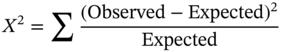
Every statistical technique has a long and interesting history. Studying how to numerically and graphically analyse the association between categorical variables is no exception. The contributions of some of the most influential statisticians, including Karl Pearson, R.A. Fisher and G.U. Yule, have left an indelible imprint on how categorical data analysis is performed. Excellent descriptions on the historical development of categorical data analysis, in particular the analysis of contingency tables, can be found by referring to, for example, Goodman and Kruskal (1954) and Agresti (2002, Chapter 16). The influence of the early pioneers has led to almost countless statistical techniques that measure, model, visualise and further scrutinise how categorical variables are related to each other. Much of the key focus has been on the numerical assessment of the strength of the association between the variables – whether the analysis is concerned with two, three or more variables. Yule and Kendall (1950), Bishop et al. (1975) and Liebetrau (1983) also provided excellent discussions of a large number of measures of association for contingency tables. The most influential and widely adopted statistical technique for analysing the association between categorical variables is Pearson’s chi-squared statistic (Pearson 1904). The importance and wide applicability of this statistic has been discussed vigourously throughout the literature – see, for example, Lancaster (1969) and Greenwood and Nikulin (1996). The statistic, simply put, is defined as where “Observed” refers to the observed count made in each cell of a table and “Expected” is its expected value under some model (even if that model reflects independence between the variables). While this statistic can detect if there is a statistically significant association between the variables it does not say anything more about the structure of the association. Various techniques may be considered for examining exactly how the association is structured. These include simple measures such as the product moment correlation (Pearson 1895) which will not only determine the strength of the association but also its direction. Model based approaches such as log-linear models and logistic models are commonly taught as a means of numerically assessing the nature of the association.
Despite the importance of modelling in statistics and her allied fields, there are two issues that need to be considered. Firstly, elementary statistics courses worldwide
teach students about the importance of visualising the structure of the data as a means of “seeing” what it looks like before resorting to inferential techniques; this might be through constructing a bar chart, histogram or boxplot of the data. However, in practice many statistical categorical analysis techniques (of course, not all) ignore this visual component altogether and go straight to modelling the structure. Secondly, modelling techniques rely on methodological assumptions of the data, or the perceived behaviour of the data by the analyst. Such thoughts are elegantly, and simply, captured in George Box’s (1979) famous quote
All models are wrong but some are useful
Earlier, Box (1976) had said
Since all models are wrong, the scientist cannot obtain a “correct” one by excessive elaboration.
Of course, such general phrases have caused a stir amongst the statistical community since a model can never fully capture the “truth” of a phenomenon. We certainly see many advantages in the wide range, and flexibility, of models that are now available but we urge caution when adopting some of them.
An alternative philosophy that can be adopted for assessing the association between the variables of a contingency table is to explore how they are associated to each other by visualising the association. There is now a plethora of strategies available for visualising numerical and categorical data. Some of the more popular approaches include the mosaic plot (Friendly 2000, 2002; Theus 2012), the fourfold display (Fienberg 1975) and the cobweb diagram (Upton 2000). The interested reader may also refer to Gabriel (2002) and Wegman and Solka (2002) for the visualisation of multivariate data. The key features of any graphical summary are that what is produced is simple, easy to interpret, and provides a quick and accurate visual representation of data. Cook and Weisberg (1999, p. 29) say of any graphical summary
In statistical graphics, information is contained in observable shapes and patterns. The task of the creator of a graph is to construct an informative view of the data that is appropriately grounded in a statistical context. The task of the viewer is to find the patterns, and then to interpret their meaning in the same context. Just as an interpretation of a painting or drawing requires understanding of the artist’s context, interpreting a graph requires an understanding of the statistical context that surrounds the graph. As in art, conclusions about a graph without understanding the context are likely to be wrong, or off the point at best.
A very good example of the interplay between data visualisation and statistical context can be found by considering Anscombe’s quartet (Anscombe 1973). While discussing his point in terms of simple linear regression, Anscombe (1973) provided a compelling argument for the need to visualise data by highlighting four very
different scatterplots with equal correlations and equal parameter estimates from a simple linear regression model. His argument shows that the context of the statistical technique needs to be made in terms of the data being analysed, and a visualisation of this context can help the analyst to better understand the statistical and practical contexts of the data being analysed.
1.2 Correspondence Analysis in a “Nutshell”
So where does correspondence analysis fit into this discussion? It is first important to recognise that often the first task in assessing the association structure between categorical variables is to either model, or measure this association, with the structure reflected in the sign and magnitude of a numerical measure. However, as we shall explore in this book, correspondence analysis (in a nutshell) provides a way to visualise the association between two or more categorical variables that form a contingency table. In doing so we gain an understanding of how particular categories from the same variable, or from different variables, “correspond” to each other. From such visual summaries, one can better understand how the variables (and categories) under inspection are associated. In doing so, the analyst can then refine their research question and postulate other structures that may exist in the data. This is all undertaken without the need to make any assumption about the structure of the data, nor does one need to impose untestable, unnecessary, or unnecessarily complicated assumptions on the data (or on the technique). The analyst, whether they are of a technical or practical persuasion, need not rely on a suite of numbers to interpret the association between the variables (unless they want to of course). Therefore, correspondence analysis is a technique that allows the data to inform the analyst of what it is trying to say rather than the model defining how the structure may be defined. The philosophy of letting the “data speak for itself” in correspondence analysis harks back to Jean-Paul Benzécri and his team at the University of Paris, France. Thus, Benzécri is considered to be the father of correspondence analysis although, in truth, many of the technical (and not visual) features stem back to earlier times. Since the early work of Benzécri and his team, the development of correspondence analysis and its many variants has been dominant in many parts of the European statistical, and allied, communities. This is especially so in France, Italy, The Netherlands and Spain. Outside of Europe, it has developed due to the contribution of researchers in Great Britain, Japan and, to a lesser extent, the USA. Unfortunately, in the Australasian region, correspondence analysis has not received the same level of attention as other parts of the world.
Before we continue with our discussion of correspondence analysis, it is worth highlighting that there are many excellent texts on its historical, computational, practical and theoretical development. The first major work that helped to expose correspondence analysis to the English speaking/reading statistical world was that of Hill (1974). Interestingly, he titled his paper “Correspondence analysis: A neglected multivariate method” which was published in the Journal of the Royal
Statistical Society, Series C (Applied Statistics). Since then, the growth of correspondence analysis has been quite slow but further insight was made 10 years later with the publication of a book by Michael Greenacre. This book, titled Theory and Applications of Correspondence Analysis was published by Academic Press and remains the most cited book of all on the topic and brought correspondence analysis out of the (mainly) French statistical literature and exposed it to the vast English reading/speaking research community; it is thus considered a landmark publication in correspondence analysis. Another excellent book is that of Lebart et al. (1984). Other books that describe the various technical and practical issues of correspondence analysis include, but are definitely not limited to, Greenacre and Blasius (2006), Greenacre (2017), Weller and Romney (1990), Gifi (1990), Benzécri (1992), Clausen (1998), Le Roux and Rouanet (2004), Murtagh (2005), Nishisato (2007) and Kroonenberg (2008) . A more recent, technical and historical overview of the variety of correspondence analysis techniques can be found in Beh and Lombardo (2014).
1.3 Data Sets
To describe correspondence analysis, and its key features, we shall be studying its application to a number of contingency tables from a variety of disciplines. In fact, much of the popularity of correspondence analysis rests with its application, not with its technical development. To attest to this, a generic title/abstract/keyword search for “correspondence analysis” on Scopus yields (as of 29 September 2020) 12385 articles concerned with correspondence analysis from the year 2000 onwards. Most recently, 900 publications can be found for the year 2019, in 2018 this number was 832, while 2017 saw 836 publications including this phrase. The most cited article was that of Ter Braak (1986) with 4281 citations followed by Hill and Gauch Jr (1980) with 2805 citations. Both these articles are written with biological/ecological researchers in mind and each propose a variant of the classical approaches to correspondence analysis technique; although we shall not be discussing these variants here.
1.3.1 Traditional European Food Data
Consider the study undertaken by Guerrero et al. (2010) and examined by Beh et al. (2011). The data stems from a study undertaken to see how the word “traditional” (from a food perspective) was perceived across six regions in six European countries; Flanders in Belgium, Burgundy (Dijon) in France, Lazio in Italy, Akershus and Ostfold in Norway, Mazovia (Warsaw) in Poland and Catalonia in Spain. There were two variables of interest in their study. The first was the Country where a participant originated from. The second variable, defined here as Freeword, consists of a list of 28 words that the recipients were asked to freely associate (that is, no prompting was given) with how they perceived traditional European food; this list was created from more complete list consisting of 1743 valid words.
Note that we shall dispense with the quotation marks (“ ”) around “traditional” for the remainder of this book.
The data is summarised in Table 1.1 and is based on the six histograms in Figure 1 of Guerrero et al. (2010). They also give an excellent and comprehensive description of the methods used to collect the data and the correspondence analysis that was originally performed using the data from their histograms.
Table 1.1 Cross-classification of Country of origin of the participants and the 28 most common Free-words that they associate with traditional European food.
Source: Based on Guerrero, L., Claret, A., Verbeke, W., Enderli, G., Zakowska-Biemans, S., and Vanhonacker, F. (2010). Perception of traditional food products in six European countries using free word association. Food Quality and Preference, 21:225–233.
Table 1.2 Temperature by Month in La Guardia airport, .
1.3.2 Temperature Data
Chambers et al. (1983) consider a range of data sets including meteorological data that were collected from the New York State Department of Conservation and the National Wildlife Service. Readings were recorded of ozone, solar radiation, wind and temperature over 152 consecutive days; the collection period was 1 May 1973 to 30 September 1973 (inclusive). Here we shall focus on the association between Temperature (measured in Fahrenheit at La Guadia airport, New York) and Month (May, June, July, August and September).
The data summarised in Table 1.2 were obtained from the data file airquality that is one of the many default data sets in R. The only variation to the data that we have made when cross-classifying the two variables is to replace the numerical labels that were originally given to each month of the study with the name of the month. Refer to Chapter 4 for more details on the analysis of this data.
1.3.3 Shoplifting Data
Consider the shoplifting data summarised in Table 1.3 which contains, in part, the results of a survey undertaken by the Dutch Central Bureau of Statistics (Israëls 1987). They were obtained from a sample of 20819 males who were suspected of shoplifting in Dutch stores between 1977 and 1978. Table 1.3 is a cross-classification of the Item stolen (the row variable) and the Age groups of the perpetrators (the column variable).
One may treat the association between Age and Item to be asymmetric such that Age is treated as the predictor variable, consisting of 13 categories, and Item is the response variable consisting of nine categories. The items categories are clothing, accessories, tobacco and/or provisions, stationary, books, records, household goods, candy, toys, jewelry, perfume, hobby and/or tools and other items; note that
the items listed here have been given labels in Table 1.3 that are in condensed form. The predictor (column) variable consists of the following nine age groups (in years) of the male perpetrators; less than 12 years ( ), 12 to 14 years (13), 15 to 17 years (16), 18 to 20 years (19), 21 to 29 years (25), 30 to 39 years (35), 40 to 49 years (45), 50 to 64 years (57) and at least 65 years ( ).
We shall be investigating how the Age of the perpetrators impacts upon their preference for shoplifting each Item; such an association structure is deemed to be asymmetric. Section 1.4 provides an interpretation of categorical variables having an asymmetric association. We shall also be examining further the nature of this association using a variant of correspondence analysis in Chapter 5 called singly ordered non-symmetric correspondence analysis.
Table 1.3 Men’s shoplifting data: Item stolen versus mid-point of the perpetrator’s Age interval.
1.3.4 Alligator Data
For an exploration of some of the issues concerned with the application of correspondence analysis for multivariate categorical data, we shall confine our attention (for the sake of simplicity) to studying the association among three categorical variables. The data we shall examine is summarised in the contingency table of Table 1.4 and comes from Agresti (2002, p. 270). It crossclassifies the Size of 219 alligators, their primary Food of choice (found in the
alligator’s stomach) and the Floridian Lake in which they reside. The four lakes are Lakes Hancock, Oklawaha, Trafford and George. This data originally came from a study undertaken by the Florida Game and Fresh Water Fish Commission and Agresti (1997, p. 270) notes that this data came from an unpublished manuscript. The interested reader may also refer to Delany and Abercrombie (1986) for earlier data related to a similar study undertaken between 1981 and 1983 from three different lakes that are within 28 km of Gainsville, Florida. The size of the alligators studied in Table 1.4 has been labelled large (for those exceeding 2.3 metres in length) and small (for those that are no more than 2.3 metres in length). Agresti (1997, p. 268) notes that the five food choices include the following. For alligators whose primary choice of food was defined as being invertebrate, they include those whose stomach contained apple snails, aquatic insects and crayfish. For those whose preferred food choice was reptile, their stomachs primarily contained turtles while the stomach of one alligator contained tags of 23 baby alligators that were released the previous year. A category bird was defined for those alligators whose stomachs contained the remains of bird wildlife while the category other refers to the alligators whose primary choice of food consisted of amphibians, mammals, plant material, stones or other debris or no food at all.
Table 1.4 Cross-classification of 219 alligators by their Size, primary Food of choice and Lake of residence. Source: Modified from Agresti, A. (2002). Categorical Data Analysis (2nd ed). Wiley, New York.
Primary Food of Choice
1.4 Symmetrical Versus Asymmetrical Association
Throughout this book we shall be examining two different types of association structure for our visualisation of the association between categorical variables. The distinction we make is on whether the categorical variables are symmetrically or asymmetrically associated. When using these two terms, we shall treat their association structure to be defined as follows:
Symmetrical association exists when all variables of the contingency table are treated as a predictor variable so that none of them are considered to be a response variable. This definition applies to the analysis of the association for contingency tables formed by cross-classifying two or more categorical variables and is the most commonly adopted type of association structure considered in the analysis of contingency tables.
Asymmetrical association exists when one variable is treated as a response to a second (or multiple) variable(s) that is (are) treated as a predictor variable. While most statistical, and practical, treatments of categorical data treat two such variables as having a symmetrical association there may be practical, or intuitive, reasons for treating the variables as exhibiting an asymmetrical association.
We will adopt these definitions of symmetrical and asymmetrical association by keeping in mind the contingency tables discussed above. For example, a symmetrical association of Country and Free-word in Table 1.1 considers that neither is treated as a response variable of the other. However if one were to assume that it is known in which Country an individual resides, then this information can be used to assess how Country impacts upon their perception of traditional European food. Therefore, we may treat the association between the two variables of Table 1.1 as being asymmetrical. In such a case, Country is treated as a predictor variable while Free-word is treated as the response variable. When quantifying the association between variables that are treated as being symmetrically associated, Pearson’s chi-squared statistic is commonly used and is the most appropriate measure to consider. However, when studying the asymmetrical association between two variables alternative measures of association must be used. Obviously, with two different association structures that we are considering in the following chapters, this will impact not only how the association between the variables is to be quantified but it also defines the type of correspondence analysis that will be performed.
For the three-way contingency table of Table 1.4 there are a variety of ways in which an analyst can study the association among the three variables. For example, we may consider the following scenarios:
1. Suppose we know from which Lake an alligator comes, and measuring its length determines its Size. Given this information we can determine the most likely primary Food of choice of the alligator without cutting open its stomach.