Oceanography and Marine Ecology, Field Director – François Lallier
Oceans
Evolving Concepts
Guy Jacques Paul Tréguer Herlé Mercier
First published 2020 in Great Britain and the United States by ISTE Ltd and John Wiley & Sons, Inc.
Apart from any fair dealing for the purposes of research or private study, or criticism or review, as permitted under the Copyright, Designs and Patents Act 1988, this publication may only be reproduced, stored or transmitted, in any form or by any means, with the prior permission in writing of the publishers, or in the case of reprographic reproduction in accordance with the terms and licenses issued by the CLA. Enquiries concerning reproduction outside these terms should be sent to the publishers at the undermentioned address:
ISTE Ltd
John Wiley & Sons, Inc.
27-37 St George’s Road 111 River Street London SW19 4EU Hoboken, NJ 07030
The rights of Guy Jacques, Paul Tréguer and Herlé Mercier to be identified as the authors of this work have been asserted by them in accordance with the Copyright, Designs and Patents Act 1988.
Library of Congress Control Number: 2020933345
British Library Cataloguing-in-Publication Data
A CIP record for this book is available from the British Library
3.2. From the chemical composition of seawater to that of plankton
3.3. Chemical tracers and water mass identification
3.4. Advancement of concepts on the pelagic ecosystem
3.5. Vertical nutrient inputs and coastal upwellings
3.6. Nutrient upwelling and Southern Ocean
3.7. Rise of marine biogeochemistry
3.8. From local nutrient inputs to large-scale ocean–atmosphere
3.9.
Chapter 4. From Marine Biology to Biological Oceanography
4.1. The key role of marine stations
4.2. The beginnings of marine ecology
4.3. A case study: a comparative approach to phyto- and zooplankton
4.3.1. Progress in phytoplankton analysis
4.3.2.
4.3.3. Progress in zooplankton
4.4. The rise of marine genomics
4.4.1. The starting point: the search for picoplankton
4.5.
4.4.2. Marine genomics, biodiversity and biotechnology
5.1.
5.1.1.
5.2. Eutrophication and anoxia of
5.2.1.
5.2.2.
5.3. Hydrothermal ecosystems
5.3.1.
5.3.2.
5.3.3. The epic of underwater
5.3.4. In the deepest depths, autonomous vehicles
5.3.5. In deep water, continuous
5.3.6.
5.3.7. Toward
5.4.
Chapter 6. A Warmer, More Acidified and Less Oxygenated Ocean
6.1. Ocean “acidification”: process, evolution and impacts ..........
6.1.1. From acidity to pH of seawater and carbonate chemistry .....
6.1.2. Variations in ocean pH over geological eras
6.1.3. Decrease in ocean pH during the industrial era
6.1.4. Decrease in pH and disturbances to the carbonate system .....
6.1.5. Impact of acidification on acoustics
6.1.6. Impact of acidification on organisms and ecosystems
6.1.7. Impact of acidification on corals ....................
6.2. A less productive ocean? ...........................
6.2.1. What are the impacts of climate change on primary production? ............................
6.2.2. What are the impacts on carbon export to the deep ocean? ...
6.2.3. A biological carbon pump activated by climate change?
6.2.4. A deep deoxygenated ocean?
6.2.5. What are the impacts on plankton?
6.3. Impacts of climate change on the ocean ...................
6.3.1.
6.4.
6.3.2.
7.1. Reminder: the ocean on a
7.2.
7.2.1.
7.2.3.
7.2.4.
7.3.
7.3.1. Elements of ocean physics at the meso- and submesoscale
7.3.2. Frontogenesis and dynamics at the submesoscale
7.3.3. High-resolution
7.3.4. Impact of mesoscale structures on upper trophic
7.3.5. Impact of the submesoscale on ecosystem structure
7.3.6. Integrating submesoscale dynamics into general circulation models ...........................
7.3.7. Incorporating diversity into physical–biogeochemical–ecosystem models
7.4.
8.2. Combining the exploitation of biological resources and sustainable development?
8.3. Combining the exploitation of deep sea mineral resources with biodiversity conservation?
8.4. Mitigating the anthropogenic greenhouse effect by manipulating the ocean?
8.4.1.
8.4.2.
8.4.3.
Acknowledgments
The authors would like to thank all those who, through review, advice, the donation of photographs, etc., have helped to produce this book, which we hope is also a tribute to a whole generation of researchers, engineers and technicians who, for half a century, have contributed to the emergence of the science of oceanography. We also would like to thank Delphine Binos, Claude Courties, Philippe Cury, Marta Estrada, Serge Garcia, Jean-Pierre Gattuso, Patrice Klein, Aline Fiala, Frank Lartaud, Odile Levrat, Marian Melin, Marc Picheral, Philippe Pondaven, Suzanne Razouls, Pascal Rivière, Bernard Salvat, Pierre-Marie Sarradin, Myriam Sibuet and Olivier Thébaud.
Published in the new Sciences encyclopedia launched in 2020 by ISTE Ltd, this book aims to introduce readers to key themes in oceanography and marine ecology by focusing on how concepts are evolving. First, we briefly recall (see Chapter 1) some elements of the history of oceanography, the birth of which is conventionally dated by the expedition of the British ship Challenger (1872–1876). The main concern of ocean physicists at that time was to understand ocean circulation and characterize ocean water masses at the basin scale and then, through major international programs, at the scale of the global ocean. With the creation of new tools, physical oceanography has gradually evolved toward describing and modeling ocean variability at different scales and studying its interactions with the atmosphere within a context of climate change (see Chapter 2). Chemical oceanography, also born with the voyage of the Challenger, after a phase dominated by analytical chemistry for the determination of seawater elements and their stoichiometry, has evolved toward biogeochemistry through the development of concepts at the interface between physics, chemistry, biology and geology to understand the relationships between nutrients and major ocean cycles in relation to the atmosphere (see Chapter 3). Biological oceanography, which originated in the 19th Century in marine stations in the coastal environment, has spread to the wider ocean, developing concepts in marine ecology, in particular to explain how pelagic biomes work. The impact of the genomic approach is overturning traditional concepts in marine biology, particularly with regard to biodiversity and functions often expressed at the cellular level (see Chapter 4). About 2.4 billion years ago, the composition of the two fluid envelopes of planet Earth underwent a drastic change, with the “great oxidation event”, leading to significant changes in ocean chemistry that had previously been displaced toward lower oxidation/reduction “redox” potentials, typical of anoxic environments. The Challenger expedition had dealt a final blow to the idea of an abiotic ocean beyond the first 500 m. In the 20th Century, one of the major discoveries was that of hydrothermal oases in ocean
ridges, showing that anoxia could go hand in hand with the production of organic matter by chemosynthesis (see Chapter 5).
While the Challenger expedition marked the birth of oceanography, this discipline has experienced, since the 1960s, a real “golden age” on a global scale with the massive recruitment of researchers, the launch of dedicated vessels and underwater vehicles, the emergence of international programs, technical revolutions (bathythermograph, automatic nutrient salt analyzers, instrumented buoys, chromatography for pigment analysis, etc.), the satellite revolution concerning a growing number of parameters and an increasingly interdisciplinary approach. The time is therefore right to combine these advances.
The last three chapters of this book go beyond the traditional routes of oceanography works. First, they attempt, through an interdisciplinary approach, to anticipate the future of a warmer, more acidified and less oxygenated ocean in the context of climate change. This is due to anthropogenic emissions of greenhouse gases, in particular carbon dioxide, more than a quarter of which is captured in the ocean, but at the cost of changing the chemical balance of carbonates (see Chapter 6). They then show how our ability to observe the ocean, not only on a large scale but also on a small scale, changes our understanding of the processes that control its functioning, physically, chemically and biologically (see Chapter 7). Finally, we present (see Chapter 8) three challenges the oceans face in the 21st Century:
– Can we exploit biological resources within the framework of sustainable development?
– Is the exploitation of its deep mining resources compatible with respect for the biodiversity of the seabed?
– Should the ocean be manipulated to better regulate climate change?
1 The Challenger Expedition: The Birth of Oceanography
1.1. The Challenger cruise (1872–1876)
It is to Great Britain’s credit that the first major oceanographic expeditions were organized, thus confirming its undeniable supremacy over the oceans (Rule, Britannia!).
One name came to be highly recognized at the end of the 19th Century, the English naturalist Charles Wyville Thomson (see Box 1.1). For many (Deacon 2001), the circumnavigation of the HMS Challenger he commanded between 1872 and 1876 marked “Year 1” of offshore oceanography. This multidisciplinary expedition sponsored by the Royal Society of London is the most expensive ever undertaken, at a cost of about 10 million pounds today.
It is true that Great Britain was at the height of its maritime domination and could not bear the idea of the United States, Germany or Sweden taking the lead. Let us examine the contributions of this circumnavigation of 68,916 miles across all oceans to the far reaches of the Southern Ocean using sails for transit and the steam engine at stations, especially for dredging.
This expedition with precise objectives (Corfield 2003) was out of the ordinary due to the meticulous preparation of the ship. Eighteen months were needed to select the old, 70-m, three-masted warship, set up laboratories and housing, winches and oceanographic equipment to study the distribution of pelagic fauna, collect organisms living at depth, multiply bathymetric measurements and take water samples at all depths.
The English naturalist Charles Wyville Thomson (1830–1882, Linlithgow), fascinated by crinoids, true living fossils, confirmed that life is abundant and diversified up to a depth of at least 4,500 m and that there is a deep ocean circulation. He published his results in The Depths of the Sea (1873), the first book dealing with the great depths, which made him the true founder of modern oceanography. He was entrusted by the British navy with the direction of the Challenger cruise and was knighted upon his return in 1876.
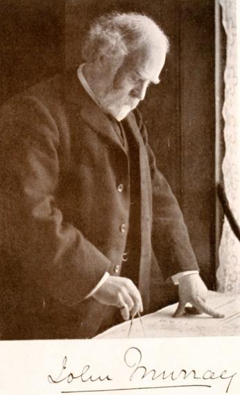
John Murray (1841, Cobourg–1914, Kirkliston) (see Figure 1.1), a man capable of all during this cruise, was responsible for the publication, at the British government’s expense, of the 50 volumes published between 1880 and 1895. With quite a bit of humor, Murray wrote in the introduction: “Our knowledge of the ocean was, in the strict sense, superficial.” In 1912, he published with the Norwegian Johan Hjort The Depths of the Ocean (1912), whose first chapter summarizes the history of oceanography from its origins. He was also knighted in 1898.
Box 1.1. Charles Wyville Thomson and John Murray
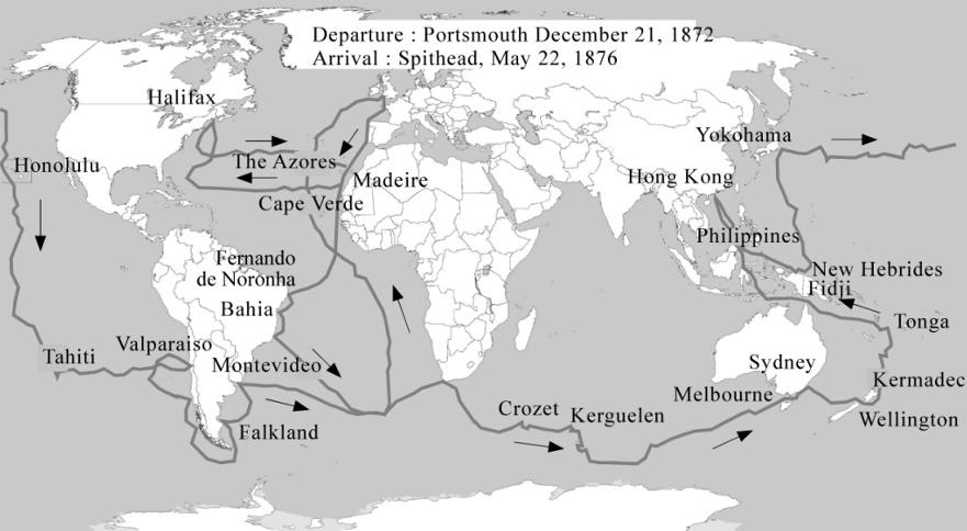
This mission was considered exceptional due to its significant number of staff. When the Challenger left Portsmouth on December 21, 1872, it had 243 officers, crew and scientists on board.
The head of the mission, Scotsman Wyville Thomson, was not in good health and returned exhausted from this journey. John Murray, another Scot, in charge of studying deep sediments, was a skillful and vigorous man. The Scot John Buchanan, a chemist, irascible and pretentious, was the genius of DIY and invention. Henry Moseley, a true naturalist, also an astronomer, was assisted by the German Rudolph von Willemoes-Suhm, who died during one of the first stops. John Wild was the expedition’s secretary and artist.
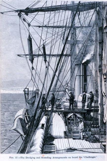
The monotony of the soundings and dredgings (see Figure 1.2) during the Challenger’s journey (see Figure 1.3) led to a number of defections by the crew: about 60 abandoned the voyage and about 10 died.
Figure 1.3. “Around the world” trip of the Challenger between December 21, 1872 and May 24, 1876
Still out of the ordinary, the 713 days at sea allowed 362 “stations”: determination of depth, meteorological conditions, direction and speed of the surface current, sampling of the surface layer of the sediment, sampling of bottom water and measurement of its temperature. In addition to most stations, plankton sampling by hauls of net and bottom dredging and trawling with beam trawls were carried out.
This expedition marked the beginning of oceanography because of its major contributions to ocean knowledge:
1) It definitively put an end to the theory of the British naturalist Edward Forbes (1843) who had stated that there could be no life beyond 400 m. Certainly, as early as 1861, the rise of a telegraph cable immersed 1,800 m at the bottom of the Mediterranean on which solitary corals had settled had already eroded this hypothesis (not to mention the forgotten work of the pharmacist and naturalist from Nice Antoine Risso in Histoire naturelle des crustacés des environs de Nice, published in 1816);
2) Of the 7,000 species harvested, about 1,500 were new; showing the richness and diversity of the deep environment, which Thomson (1873) translated into these terms: It is inhabited by a fauna more rich and varied on account of the enormous extent of the area, and with organisms in many cases apparently even more elaborately and delicately formed and more
exquisitely beautiful, in their soft shades of coloring and the rainbow tints of their wonderful phosphorescence, than the fauna of the wellknown belt of shallow water.
3) It specified the topography of the seabed showing a depth of more than 8,183 m in the Mariana trench (the Challenger did not have a longer cable!) and highlighted the mid-Atlantic ridge, thus preparing the way for Alfred Wegener’s (1912) continental drift theory;
4) It showed that sediments were formed from pelagic organisms: globigerin, diatomaceous earth, pteropod and red mud from the deep sea;
5) It brilliantly confirmed the constancy of the relative proportions of the various salts contained in seawater, having been previously observed in 1819 by the Swiss Alexandre Marcet and, in 1855, by the American Matthew Fontaine Maury. We will elaborate on this at the beginning of Chapter 3.
Carpenter’s hope to discover the mechanisms of ocean circulation was not materializing, despite valuable information gathered on vertical profiles of temperature, salinity and density, including confirmation that cold waters (2°C) found near the bottom in the vicinity of Fernando de Noronha formed on the surface and in winter in the North Atlantic. This partial success was due to the absence of a real physicist, the poor quality of the thermometers (maximum-minimum temperature produced by Mille-Casella, then Negretti and Zambra, and Richter and Wiese reversing thermometers), the inadequacy of British meteorology and the lack of knowledge of fluid mechanics at that time.
The return to Great Britain did not mark the end of the adventure. Thomson set up a study in Edinburgh to collate the data, distribute the specimens and supervise the publication of the results, which lasted 23 years for 50 volumes and 30,000 pages written by many scholars under the supervision of John Murray (Thomson and Murray 1885–1895). This period was marked by quarrels between the British Museum, which wanted to coordinate this synthesis, English researchers, who wanted exclusivity, and the Treasury, who was reluctant to pay an ever-increasing bill.
1.2. From the Challenger to the “golden age” of oceanography
As our book shows the development of concepts essentially between 1960 and today, we would not want to abandon the Challenger by suggesting that there was nothing between this expedition and the “golden age” of oceanography. On the contrary, many cruises enabled the development of concepts and methods. Georg
Wüst (1964) listed about 20 oceanographic cruises between 1873 and 1960 and, with less strict criteria, François Carré (2001) counted between 110 and 115 between 1900 and 1956 with increasing frequency after the Second World War when Germany disappeared into the background and the United States and the USSR moved to the foreground. These cruises remained national for political or economic reasons (northern shipping route, fishing, whaling). Twelve countries participated in this expansion, with only eight being present throughout the period: Argentina, Belgium, Canada, Denmark, France (including Monaco), the Netherlands, Sweden and the United Kingdom. The practice of oceanography by enlightened and wealthy individuals on board their yachts (Alexandre Agassiz, John Buchanan, Albert I of Monaco [see Figure 1.4], King Don Carlos of Portugal, the Duke of Orléans and Jean Charcot) disappeared due to financial requirements and the institutionalization of research.
The first cruises, centered on hydrography, were carried out on national marine vessels (Challenger, Gazelle, the first Vitiaz) before oceanographers had their own units. The American ship Albatross, a steel steamship made available to the United States Fisheries Commission in 1883, was the first specifically built for research. With the era of generalist cruises over, it is interesting to examine the dominant themes of this period. From 1900 to 1939, the focus was on three areas: bathymetry, water mass structure and movements, and species inventory and distribution. From
1945 to 1956, the cruise focused on depths: geology, geophysics and biology. The world tour of the Swedish Albatross in 1947–1948, as close as possible to the equator, allowed, because of the Kullenberg corer, sediment samples about 20 m thick to be taken, that is as far back as the cenozoic era. The cruises of the Danish Galathea and the American Vema, a 70-m yacht transformed into a research vessel, under the direction of Maurice Ewing, completed this study of large trenches.
High latitudes were beginning to fascinate because of strategic and geopolitical issues, particularly the southern hemisphere with the Belgian cruise of Belgica and Scotland with Scotia, England with Discovery and France with the Français and the Pourquoi Pas? of Commander Charcot. The importance of the Southern Ocean in the global ocean system was beginning to become apparent, hence an effort by the British (William Scoresby and Discovery II) and Norwegians (Norvegia and Torshavn), and later, at the end of the Second World War, the United States and the USSR came on board. The Arctic was also not forgotten, especially following the second International Polar Year of 1933, mainly by Russians interested in the Northern Sea Route.
2 From Physical Oceanography to Ocean–Atmosphere Interactions
Observing the oceans allows us to describe their state and the variability of their physical, biogeochemical and biological components. From this knowledge, questions emerge about the major balances underlying each of these compartments that require theories and models to be answered.
Since the Challenger’s expedition, the need to better understand these compartments has been the driving force behind instrumental developments that have gradually revealed the complexity of the ocean and now provide observation systems, both in situ and from space, that allow the oceans to be monitored. The task is immense: to characterize the spatial variability of the ocean from a local to a global scale and to track the temporal variability of the ocean on time scales ranging from a few minutes (associated with turbulence and mixing) to seasons of water mass formation to decades and centuries of natural or anthropogenic climate variability. The weakness of climate signals in the abyssal ocean, particularly those related to anthropogenic forcing, adds to the complexity and requires high-precision measurements.
In this chapter dedicated to physical oceanography, we will focus on the hydrological properties of water masses (temperature and salinity distribution as a function of position) and on ocean currents. Biogeochemical tracers, such as dioxygen, nutrients or chlorofluorocarbons, can also be used to track water bodies and determine their history, but will be discussed only briefly here. Oceans: Evolving Concepts, First Edition. Guy Jacques, Paul Tréguer and Herlé Mercier.
Technological advances revealing the complexity of the ocean
2.1.1.
Hydrological measurements
The Challenger expedition measured the temperature of water masses using reversing thermometers; this technology was used until the early 1970s. The accuracy was already very good (0.005°C), but the composition of seawater remained to be determined. This expedition allowed Dittmar (1884) to analyze 77 seawater samples to determine their salt composition. He noted that while the proportion of salts in seawater was relatively constant, the total amount of salt varied greatly from one sample to another. He thus anticipated one of the major topics of oceanography: determining the latitude, longitude and depth distribution of salinity. A definition was needed to make the measures comparable. In 1902, a commission of the ICES (International Council for the Exploration of the Sea), chaired by the German biologist Walter Herwig, proposed a definition of ocean salinity based on chlorinity.
During the Challenger’s expedition, seawater samples were taken using bottles mounted along a cable, several kilometers long, to sample the layers from the surface to the bottom. A messenger sliding along the cable caused the bottles to close and the thermometers to turn upside down. The water collected in this way was brought to the surface, transferred to bottles and then analyzed. As the number of vertical sampling bottles was limited (usually about 10), profile repetitions were necessary to sample the deepest ocean regions.
These measurements made it possible to identify the different water masses in the ocean. Wüst (1935), using data collected during expeditions on board the Meteor, traced the movement of water masses by noting that their core was defined by the extremes of properties (salinity maximum for water from the Mediterranean, for example) that can be monitored over long distances. In addition to temperature and salinity measurements, Wüst relied on dissolved dioxygen content in water measurements, measured using the Winkler method (1888).
Today, temperature and salinity measurements are carried out with CTDO2 (conductivity, temperature, depth, dissolved oxygen) probes that determine the temperature and salinity of the ocean as a function of pressure with a sampling frequency of 24 Hz and high accuracy: 1 decibar for pressure, 0.001°C for temperature, 0.002 for salinity and 1 μmol·kg 1 for dissolved dioxygen. These accuracies, for salinity and dioxygen, can only be obtained after calibration of these parameters from concentration measurements in samples taken at different points on the vertical.
In practice, it is the conductivity of the ocean that is measured and adjusted with respect to observations and then transformed into salinity. CTDO2 probes are mounted on frames (see Figure 2.1) equipped with sampling bottles and acoustic Doppler current meters to measure the current profile at the same time as the hydrological property profiles.
These advances have revealed dynamic structures such as deep western currents that had not been identified by the Challenger’s expedition but had been identified in those conducted by the World Ocean Circulation Experiment (WOCE) (see Figure 2.2). The vertical resolution made it possible to highlight structures such as density inversions, representative of double diffusion.
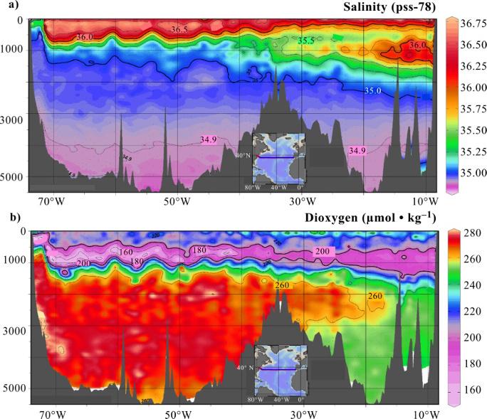
Figure 2.2. WOCE Section A03 in the North Atlantic. For a color version of this figure, see www.iste.co.uk/jacques/oceans.zip
COMMENT ON FIGURE 2.2.– Salinity (pss-78, or practical salinity scale 1978) and dioxygen along 36°N in September–October 1993. Measurements were taken along the route shown in the insert; the American coast is on the left and Europe on the right. The horizontal axis corresponds to the longitude in degrees west and the vertical axis to the depth. The scale to the right of the plots shows the correspondence between the colors and the physical units. The maximum salinity, centered at 1,000 m on the eastern shore, indicates the presence of Mediterranean water. The maximum dioxygen concentrations (red and orange) indicate water masses recently in contact with the atmosphere that originated in the Labrador Sea and northern seas (eWOCE1; Schlitzer 2000).
2.1.2. Current measurements
Surface drifting objects, such as wrecks, have long been used to estimate surface ocean circulation. It was in December 1883 that the U.S. Navy Hydrographic Bureau began publishing monthly pilot charts.
1 http://www.ewoce.org/.
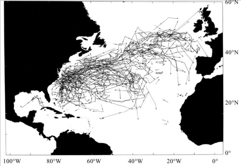
These maps reported, among other things, the surface drift of abandoned ships and other identifiable debris. The trajectories of these wrecks were compiled by Richardson (1985) (see Figure 2.3) and reveal the surface ocean circulation.
Figure 2.3. The surface drift of wrecks listed in the pilot charts between 1883 and 1902 highlights the Gulf Stream and its extension into the North Atlantic (Richardson 1985)
Surface drifting buoys have become an important element in ocean observation. It was the advent of satellite positioning and data collection, in particular the Argos system, created in 1978 as part of a Franco-American cooperation, that made it possible to deploy surface drifting buoys on a global scale (Lumpkin et al. 2017). After numerous tests, the Surface Velocity Program (now the Global Drifter Program), launched in 1979, includes a surface drifting buoy to which a floating anchor several meters long is connected, positioned at a depth of 15 m. The satellite location tracking and geographical localization system is mounted on the surface float. Surface temperature and atmospheric pressure are measured by the surface drifting buoy that currently uses GPS positioning.
Deep circulation and velocity of deep currents have long remained unknown. Oceanographers assumed, by interpreting the circulation, that the velocity at the interface between two water masses was negligible. With the idea that a drifting object could reveal circulation, but this time at depth, John Swallow (1953)
developed a float whose buoyancy was adjusted so that it drifted at a predetermined depth. The float is positioned by acoustic means.
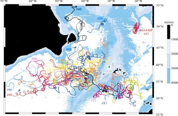
An initial experiment confirmed the existence of the Deep Western Boundary Current under the Gulf Stream, as predicted by the theoretical studies of Stommel and Arons (1959a, 1959b). The floats showed an intensified current at the bottom, with speeds of up to 17.4 cm/sec per 2,800 m of water. A second experiment (Swallow 1971) was conducted in 1960 off Bermuda over a period of 14 months. The objective was to verify whether Stommel’s prediction of a deep interior circulation of low intensity and northward direction was valid. The floats were deployed between 2,000 and 4,000 m deep and revealed an energetic circulation with currents of about 10 cm/sec. They were highly variable and associated with mesoscale vortex structures. Following this first demonstration, many experiments based on this drifting float technology were carried out, increasingly revealing the complexity of ocean circulation (see Figure 2.4).
The discovery of these medium-scale structures, the equivalent of depressions or anticyclones in the atmosphere, but with spatial scales 10 times smaller, came to occupy oceanographers during the following decade when experiments such as Mode and Polymode in 1973–1978 (The Mode group 1978) or Tourbillon (Le Groupe Tourbillon 1983) were trying to describe them.
Figure 2.4. Trajectories of 26 Sofar floats (Langrangian SOund Fixing And Ranging) that have drifted for more than 2 years in the North Atlantic between 600 and 800 m deep. The trajectories reveal the almost systematic presence of medium-scale structures with trajectories forming loops (Ollitrault and Colin de Verdière 2002a, 2002b). For a color version of this figure, see www.iste.co.uk/jacques/oceans.zip
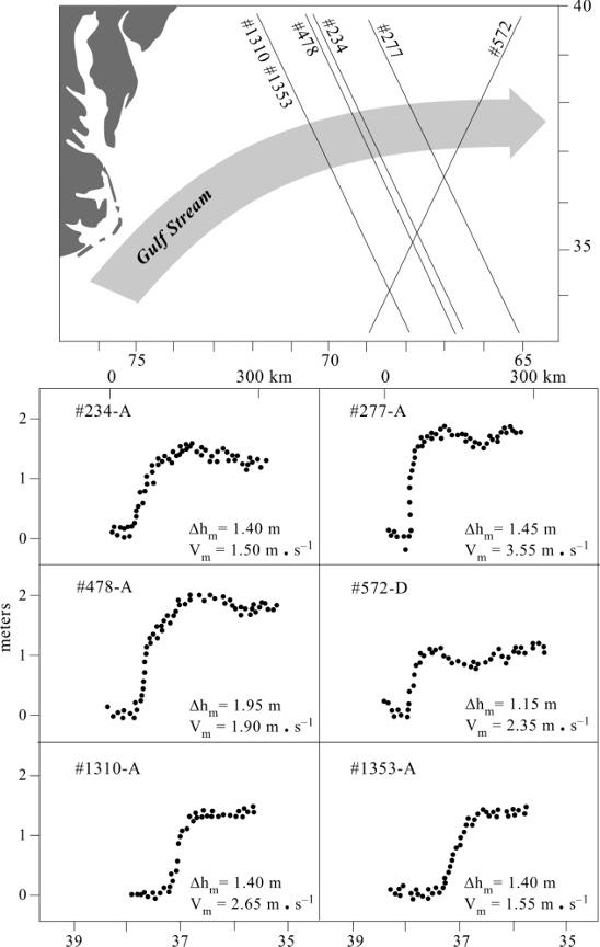
In 1978, the Seasat satellite was launched with an altimeter on board to measure the sea surface height from space. Despite a short lifetime (100 days), the satellite showed the feasibility of the measurement, showing a difference in sea surface height of about 1 m across the Gulf Stream (see Figure 2.5). This demonstration paved the way for the measurement, from space, of the dynamic topography of the ocean, and therefore of surface geostrophic currents. The variability shown by the six passes through the Gulf Stream demonstrated the transient nature of ocean eddies. At the same time, satellite measurements of sea surface temperature became available.
Figure 2.5. The Gulf Stream as seen by Seasat. (a) Ground traces of the satellite's measurements of sea surface elevation change. The position of the Gulf Stream is indicated by the arrow. (b) Sea surface variations across the Gulf Stream for the six tracks listed above. The difference in elevation, Δhm, across the Gulf Stream varies from 1.15 to 1.95 m and the associated geostrophic velocity varies between 1.50 and 3.55 m ⋅sec -1 (Kao and Cheney 1982)
Fluid mechanics applied to oceanography
2.6. Henry Stommel in 1965 on board the Atlantis II (Wunsch 1997)
Henry “Hank” Melson Stommel (see Figure 2.6) turned to oceanography at WHOI (Woods Hole Oceanographic Institution) from 1944 until 1959, with the Office of Naval Research supporting his projects. He proposed theories on global ocean circulation and Gulf Stream behavior and, in 1959, became a professor at Harvard and worked at MIT (Massachusetts Institute of Technology) before returning to WHOI in 1963 until his retirement.
Stommel became famous with the publication in 1948 of “The westward intensification of wind-driven ocean currents”, one of the most widely cited articles in physical oceanography. Based on fluid mechanics, he suggests that the rotation of the Earth (Coriolis force) explains the strengthening of Western Boundary Currents such as the Gulf Stream (in 1958 he published The Gulf Stream: Physical and Dynamic Description) or the Kuroshio (“black current” in Japanese, which underlines its oligotrophy). He also showed that this northward flow is counterbalanced by a southward cold water current flowing under the first one. With Arnold Arons, he extended his research to deep circulation, proposing a scheme where surface water dives into the polar regions to feed deep currents in the western part of the basins, while the interior flow moves toward the poles. He also developed the first thermohaline circulation models.
He was the first to carry out monthly outings for several years thanks to the wooden oceanographic vessel Palinurus from the Bermuda Biological Station. The slope of the plateau allowed him to quickly reach great depths and thus obtain profiles for temperature, salinity and other chemical data. In addition to this research on general circulation, Stommel was also interested in the classification of estuaries, turbulent diffusion and the impacts of volcanoes on climate.
Box 2.1. Henry Stommel (1920–1992)
Figure
2.2. The international TOGA and WOCE programs
Building on these instrumental developments and emerging technologies, oceanographers conducted two major programs in the 1990s: TOGA (Tropical Ocean Global Atmosphere) and WOCE, which set the basis for today’s observation systems. These two programs, which were part of the World Climate Research Program, enabled rapid progress in the acquisition of new data to better understand and then predict, using numerical models, the “climate” of the oceans.
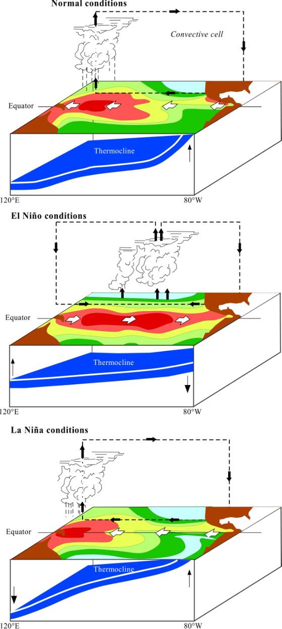
The TOGA program was motivated by the arrival, in 1982–1983, of an El NiñoSouthern Oscillation (ENSO) event of exceptional intensity (see Figure 2.7). Peru, Ecuador and the western United States experienced torrential rains causing exceptional flooding, while Indonesia and Australia experienced record droughts. However, scientists were late in understanding what was happening, when the El Niño phenomenon reached its maximum intensity in December 1982 (Cane 1983).
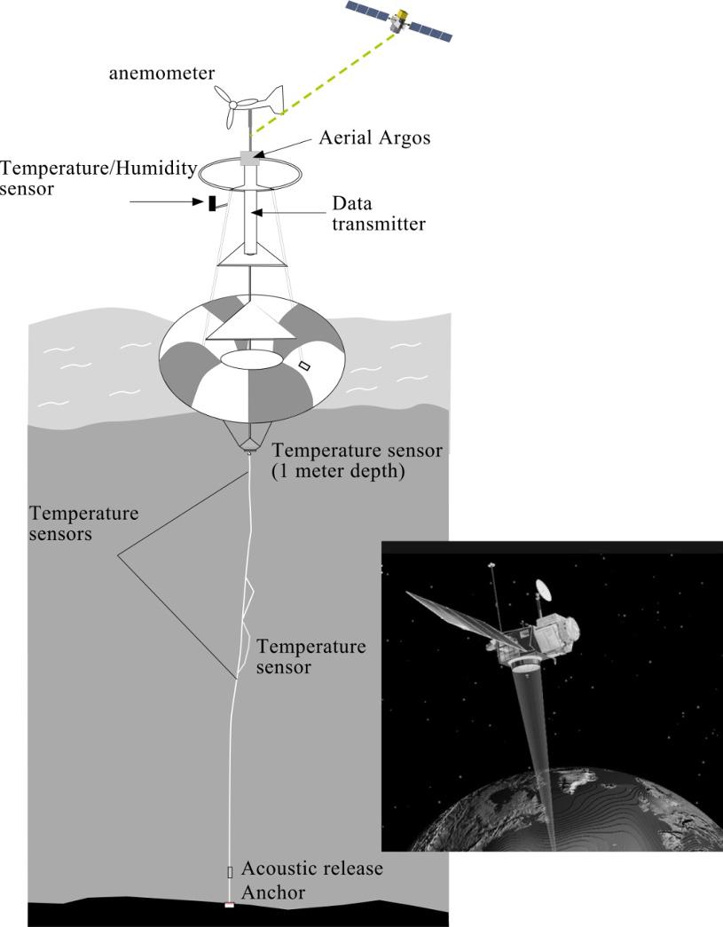
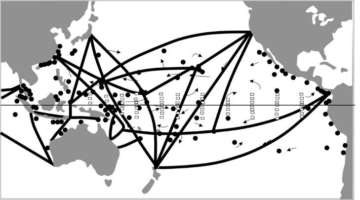
The global impacts of ENSO have motivated many efforts to understand its origin and forecast it; they are included in the TOGA program. With ENSO being an interaction phenomenon between the ocean and the atmosphere, TOGA is built to acquire a database covering both the tropical Pacific Ocean and its atmosphere. TOGA aims to develop coupled models that understand the ocean–atmosphere interaction mechanisms underlying ENSO and determine the predictability of the ocean–atmosphere system in the Pacific both seasonally and interannually (McPhaden et al. 2011). One of the key elements for observing the tropical Pacific Ocean is the Atlas buoy network, which provides meteorological, surface and subsurface oceanographic measurements (see Figure 2.8). The first deployments of these buoys were made in 1984 and the complete network of 70 buoys covering the entire Pacific was established in 1994 (see Figure 2.9). The network is complemented by other in situ observations such as XBT lines (eXpendable BathyThermograph). The program benefits from the development of ocean observation from space with the measurement of ocean surface temperature by NOAA (National Oceanographic Atmospheric Administration) satellites, altimeters providing access to sea surface elevation and ocean heat content, from Topex/Poseidon, launched by CNES (French National Centre for Space Studies) and NASA and ERS-1, launched by ESA (European Space Agency), whose scatterometer also measures ocean surface winds. TOGA data are available in real time (or near real time, with a delay of a few days), which allows the setup of forecast models. Meteorological centers, such as the NCEP (National Centers for Environmental Prediction) or the ECMWF (European Centre for Medium-range Weather Forecasts), now routinely offer an ENSO forecast.
Figure 2.7. El Niño. For a color version of this figure, see www.iste.co.uk/jacques/oceans.zip
COMMENT ON FIGURE 2.7.– The three states of ocean–atmosphere interactions in the equatorial Pacific. The surface temperature ranges from red (maximum) to blue (minimum). Under “normal” conditions, winds and surface currents are directed westward at the equator, causing cold, nutrient-rich water to upwell at the eastern boundary of the Pacific, promoting organic production. Under El Niño conditions, easterly winds weaken, the thermocline deepens and warm surface water invades the eastern Pacific. In La Niña conditions, upwelling on the eastern Pacific coast intensifies.
COMMENT ON FIGURE 2.8.– Diagram of an Atlas buoy mooring with the FrenchAmerican satellite (NASA and CNES) Topex/Poseidon launched in 1992 as part of the WOCE program, which came to benefit TOGA. Topex/Poseidon’s altimeter radar measures changes in the ocean surface height with centimeter accuracy. The observation system improved considerably during the 10 years of the program, with Atlas moorings covering the entire tropical Pacific (see Figure 2.9).
Figure 2.9. TOGA observation system in 1994: it included opportunity vessels for XBT measurement of ocean temperature between 0 and 700 m, Atlas moorings, tide gauges and surface drifting buoys (McPhaden et al. 1998)
The WOCE program (1992–1998) is probably the most ambitious ocean observation program launched to date. From the early stages of thinking about what WOCE should be, the idea was to combine satellite and in situ measurements for ocean observation on the global scale from the surface to the bottom. The challenge was immense; it was necessary to measure the dynamic topography of the ocean from space with centimeter accuracy to detect the surface signal of mesoscale eddies, the wind at the ocean surface, the physical and biogeochemical properties of the global ocean as well as the deep circulation. This challenge was intended to meet the two main objectives of the WOCE:
1) Develop models for climate change prediction and acquire the database to validate them;
2) Determine the representativeness of the WOCE dataset for long-term ocean behavior in order to find methods for determining these changes.
Taking advantage of strong international collaboration, the WOCE managed to acquire most of the planned data. An unprecedented effort was made to standardize