Introduction
Time series data is an important source of information used for future decision making, strategy, and planning operations in different industries: from marketing and finance to education, healthcare, and robotics. In the past few decades, machine learning model-based forecasting has also become a very popular tool in the private and public sectors.
Currently, most of the resources and tutorials for machine learning model-based time series forecasting generally fall into two categories: code demonstration repo for certain specific forecasting scenarios, without conceptual details, and academic-style explanations of the theory behind forecasting and mathematical formula. Both of these approaches are very helpful for learning purposes, and I highly recommend using those resources if you are interested in understanding the math behind theoretical hypotheses.
This book fills that gap: in order to solve real business problems, it is essential to have a systematic and well-structured forecasting framework that data scientists can use as a guideline and apply to real-world data science scenarios. The purpose of this hands-on book is to walk you through the core steps of a practical model development framework for building, training, evaluating, and deploying your time series forecasting models.
The first part of the book (Chapters 1 and 2) is dedicated to the conceptual introduction of time series, where you can learn the essential aspects of time series representations, modeling, and forecasting.
In the second part (Chapters 3 through 6), we dive into autoregressive and automated methods for forecasting time series data, such as moving average, autoregressive integrated moving average, and automated machine learning for time series data. I then introduce neural networks for time series forecasting, focusing on concepts such as recurrent neural networks (RNNs) and
the comparison of different RNN units. Finally, I guide you through the most important steps of model deployment and operationalization on Azure.
Along the way, I show at practice how these models can be applied to real-world data science scenarios by providing examples and using a variety of open-source Python packages and Azure. With these guidelines in mind, you should be ready to deal with time series data in your everyday work and select the right tools to analyze it.
What Does This Book Cover?
This book offers a comprehensive introduction to the core concepts, terminology, approaches, and applications of machine learning and deep learning for time series forecasting: understanding these principles leads to more flexible and successful time series applications.
In particular, the following chapters are included:
Chapter 1: Overview of Time Series Forecasting This first chapter of the book is dedicated to the conceptual introduction of time series, where you can learn the essential aspects of time series representations, modeling, and forecasting, such as time series analysis and supervised learning for time series forecasting.
We will also look at different Python libraries for time series data and how libraries such as pandas, statsmodels, and scikit-learn can help you with data handling, time series modeling, and machine learning, respectively. Finally, I will provide you with general advice for setting up your Python environment for time series forecasting.
Chapter 2: How to Design an End-to-End Time Series Forecasting Solution on the Cloud The purpose of this second chapter is to provide an end-to-end systematic guide for time series forecasting from a practical and business perspective by introducing a time series forecasting template and a real-world data science scenario that we use throughout this book to showcase some of the time series concepts, steps, and techniques discussed.
Chapter 3: Time Series Data Preparation In this chapter, I walk you through the most important steps to prepare your time series data for forecasting models. Good time series data preparation produces clean and well-curated data, which leads to more practical, accurate predictions. Python is a very powerful programming language to handle data, offering an assorted suite of libraries for time series data and excellent support for time series analysis, such as SciPy, NumPy, Matplotlib, pandas, statsmodels, and scikit-learn.
You will also learn how to perform feature engineering on time series data, with two goals in mind: preparing the proper input data set that is compatible with the machine learning algorithm requirements and improving the performance of machine learning models.
Chapter 4: Introduction to Autoregressive and Automated Methods for Time Series Forecasting In this chapter, you discover a suite of autoregressive methods for time series forecasting that you can test on your forecasting problems. The different sections in this chapter are structured to give you just enough information on each method to get started with a working code example and to show you where to look to get more information on the method.
We also look at automated machine learning for time series forecasting and how this method can help you with model selection and hyperparameter tuning tasks.
Chapter 5: Introduction to Neural Networks for Time Series Forecasting In this chapter, I discuss some of the practical reasons data scientists may still want to think about deep learning when they build time series forecasting solutions. I then introduce recurrent neural networks and show how you can implement a few types of recurrent neural networks on your time series forecasting problems.
Chapter 6: Model Deployment for Time Series Forecasting In this final chapter, I introduce Azure Machine Learning SDK for Python to build and run machine learning workflows. You will get an overview of some of the most important classes in the SDK and how you can use them to build, train, and deploy a machine learning model on Azure. Through machine learning model deployment, companies can begin to take full advantage of the predictive and intelligent models they build and, therefore, transform themselves into actual AI-driven businesses. Finally, I show how to build an end-to-end data pipeline architecture on Azure and provide deployment code that can be generalized for different time series forecasting solutions.
Reader Support for This Book
This book also features extensive sample code and tutorials using Python, along with its technical libraries, that readers can leverage to learn how to solve real-world time series problems. Readers can access the sample code and notebooks at the following link: aka.ms/ML4TSFwithPython
Overview of Time Series Forecasting
Time series is a type of data that measures how things change over time. In a time series data set, the time column does not represent a variable per se: it is actually a primary structure that you can use to order your data set. This primary temporal structure makes time series problems more challenging as data scientists need to apply specific data preprocessing and feature engineering techniques to handle time series data.
However, it also represents a source of additional knowledge that data scientists can use to their advantage: you will learn how to leverage this temporal information to extrapolate insights from your time series data, like trends and seasonality information, to make your time series easier to model and to use it for future strategy and planning operations in several industries. From finance to manufacturing and health care, time series forecasting has always played a major role in unlocking business insights with respect to time.
Following are some examples of problems that time series forecasting can help you solve:
■ What are the expected sales volumes of thousands of food groups in different grocery stores next quarter?
■ What are the resale values of vehicles after leasing them out for three years?
■ What are passenger numbers for each major international airline route and for each class of passenger?
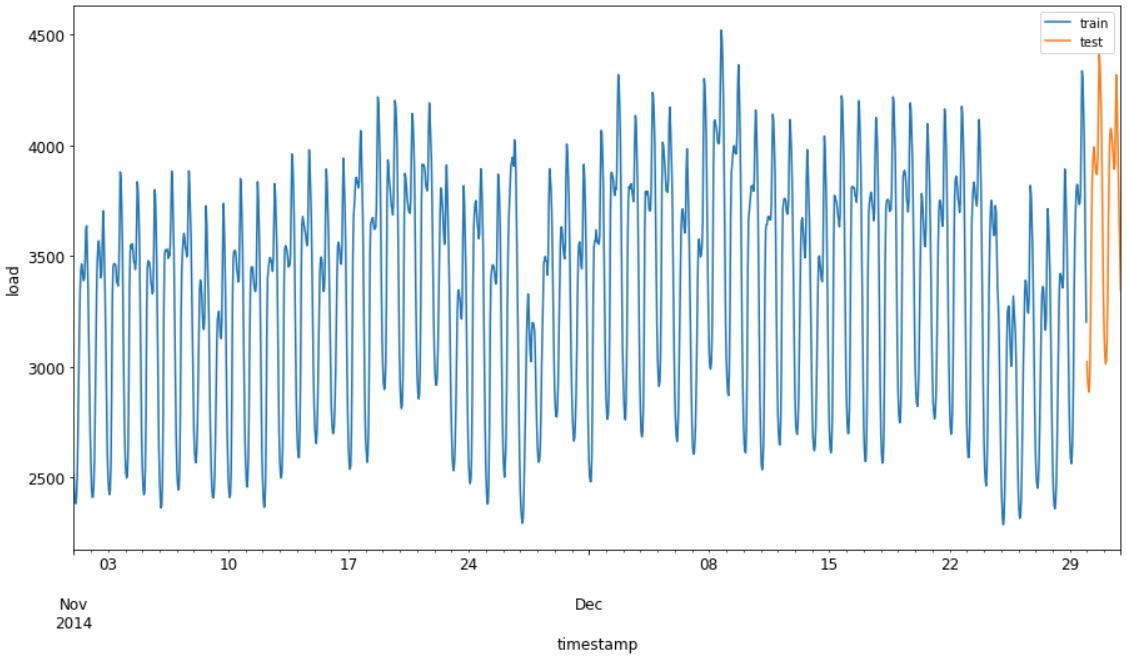
■ What is the future electricity load in an energy supply chain infrastructure, so that suppliers can ensure efficiency and prevent energy waste and theft?
The plot in Figure 1.1 illustrates an example of time series forecasting applied to the energy load use case.
This first chapter of the book is dedicated to the conceptual introduction— with some practical examples—of time series, where you can learn the essential aspects of time series representations, modeling, and forecasting. Specifically, we will discuss the following:
■ Flavors of Machine Learning for Time Series Forecasting – In this section, you will learn a few standard definitions of important concepts, such as time series, time series analysis, and time series forecasting, and discover why time series forecasting is a fundamental cross-industry research area.
■ Supervised Learning for Time Series Forecasting – Why would you want to reframe a time series forecasting problem as a supervised learning problem? In this section you will learn how to reshape your forecasting scenario as a supervised learning problem and, as a consequence, get access to a large portfolio of linear and nonlinear machine learning algorithms.
Figure 1.1: Example of time series forecasting applied to the energy load use case
■ Python for Time Series Forecasting – In this section we will look at different Python libraries for time series data and how libraries such as pandas, statsmodels, and scikit-learn can help you with data handling, time series modeling, and machine learning, respectively.
■ Experimental Setup for Time Series Forecasting – This section will provide you general advice for setting up your Python environment for time series forecasting.
Let’s get started and learn some important elements that we must consider when describing and modeling a time series.
Flavors of Machine Learning for Time Series Forecasting
In this first section of Chapter 1, we will discover together why time series forecasting is a fundamental cross-industry research area. Moreover, you will learn a few important concepts to deal with time series data, perform time series analysis, and build your time series forecasting solutions.
One example of the use of time series forecasting solutions would be the simple extrapolation of a past trend in predicting next week hourly temperatures. Another example would be the development of a complex linear stochastic model for predicting the movement of short-term interest rates. Time-series models have been also used to forecast the demand for airline capacity, seasonal energy demand, and future online sales.
In time series forecasting, data scientists’ assumption is that there is no causality that affects the variable we are trying to forecast. Instead, they analyze the historical values of a time series data set in order to understand and predict their future values. The method used to produce a time series forecasting model may involve the use of a simple deterministic model, such as a linear extrapolation, or the use of more complex deep learning approaches.
Due to their applicability to many real-life problems, such as fraud detection, spam email filtering, finance, and medical diagnosis, and their ability to produce actionable results, machine learning and deep learning algorithms have gained a lot of attention in recent years. Generally, deep learning methods have been developed and applied to univariate time series forecasting scenarios, where the time series consists of single observations recorded sequentially over equal time increments (Lazzeri 2019a).
For this reason, they have often performed worse than naïve and classical forecasting methods, such as exponential smoothing and autoregressive integrated moving average (ARIMA). This has led to a general misconception that deep learning models are inefficient in time series forecasting scenarios, and many data
scientists wonder whether it’s really necessary to add another class of methods, such as convolutional neural networks (CNNs) or recurrent neural networks (RNNs), to their time series toolkit (we will discuss this in more detail in Chapter 5, “Introduction to Neural Networks for Time Series Forecasting”) (Lazzeri 2019a).
In time series, the chronological arrangement of data is captured in a specific column that is often denoted as time stamp, date, or simply time. As illustrated in Figure 1.2, a machine learning data set is usually a list of data points containing important information that are treated equally from a time perspective and are used as input to generate an output, which represents our predictions. On the contrary, a time structure is added to your time series data set, and all data points assume a specific value that is articulated by that temporal dimension.
Now that you have a better understanding of time series data, it is also important to understand the difference between time series analysis and time series forecasting. These two domains are tightly related, but they serve different purposes: time series analysis is about identifying the intrinsic structure and extrapolating the hidden traits of your time series data in order to get helpful information from it (like trend or seasonal variation—these are all concepts that we will discuss later on in the chapter).
Data scientists usually leverage time series analysis for the following reasons:
■ Acquire clear insights of the underlying structures of historical time series data.
■ Increase the quality of the interpretation of time series features to better inform the problem domain.
■ Preprocess and perform high-quality feature engineering to get a richer and deeper historical data set.
Figure 1.2: Machine learning data set versus time series data set
Time series analysis is used for many applications such as process and quality control, utility studies, and census analysis. It is usually considered the first step to analyze and prepare your time series data for the modeling step, which is properly called time series forecasting.
Time series forecasting involves taking machine learning models, training them on historical time series data, and consuming them to forecast future predictions. As illustrated in Figure 1.3, in time series forecasting that future output is unknown, and it is based on how the machine learning model is trained on the historical input data.
Time series analysis on historical and/or current time stamps and values
01/02/2020
01/03/2020
01/04/2020
01/05/2020
01/06/2020
01/07/2020
01/08/2020
01/09/2020
01/10/2020
Time series forecasting on future time stamps to generate future values
Figure 1.3: Difference between time series analysis historical input data and time series forecasting output data
Different historical and current phenomena may affect the values of your data in a time series, and these events are diagnosed as components of a time series. It is very important to recognize these different influences or components and decompose them in order to separate them from the data levels.
As illustrated in Figure 1.4, there are four main categories of components in time series analysis: long-term movement or trend, seasonal short-term movements, cyclic short-term movements, and random or irregular fluctuations. Sensor
Figure 1.4: Components of time series
Let’s have a closer look at these four components:
■ Long-term movement or trend refers to the overall movement of time series values to increase or decrease during a prolonged time interval. It is common to observe trends changing direction throughout the course of your time series data set: they may increase, decrease, or remain stable at different moments. However, overall you will see one primary trend. Population counts, agricultural production, and items manufactured are just some examples of when trends may come into play.
■ There are two different types of short-term movements:
■ Seasonal variations are periodic temporal fluctuations that show the same variation and usually recur over a period of less than a year. Seasonality is always of a fixed and known period. Most of the time, this variation will be present in a time series if the data is recorded hourly, daily, weekly, quarterly, or monthly. Different social conventions (such as holidays and festivities), weather seasons, and climatic conditions play an important role in seasonal variations, like for example the sale of umbrellas and raincoats in the rainy season and the sale of air conditioners in summer seasons.
■ Cyclic variations, on the other side, are recurrent patterns that exist when data exhibits rises and falls that are not of a fixed period. One complete period is a cycle, but a cycle will not have a specific predetermined length of time, even if the duration of these temporal fluctuations is usually longer than a year. A classic example of cyclic variation is a business cycle, which is the downward and upward movement of gross domestic product around its long-term growth trend: it usually can last several years, but the duration of the current business cycle is unknown in advance.
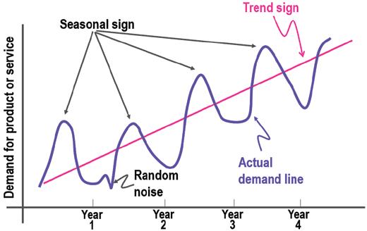
As illustrated in Figure 1.5, cyclic variations and seasonal variations are part of the same short-term movements in time series forecasting, but they present differences that data scientists need to identify and leverage in order to build accurate forecasting models:
Figure 1.5: Differences between cyclic variations versus seasonal variations
■ Random or irregular fluctuations are the last element to cause variations in our time series data. These fluctuations are uncontrollable, unpredictable, and erratic, such as earthquakes, wars, flood, and any other natural disasters.
Data scientists often refer to the first three components (long-term movements, seasonal short-term movements, and cyclic short-term movements) as signals in time series data because they actually are deterministic indicators that can be derived from the data itself. On the other hand, the last component (random or irregular fluctuations) is an arbitrary variation of the values in your data that you cannot really predict, because each data point of these random fluctuations is independent of the other signals above, such as long-term and short-term movements. For this reason, data scientists often refer to it as noise, because it is triggered by latent variables difficult to observe, as illustrated in Figure 1.6.
Data scientists need to carefully identify to what extent each component is present in the time series data to be able to build an accurate machine learning forecasting solution. In order to recognize and measure these four components, it is recommended to first perform a decomposition process to remove the component effects from the data. After these components are identified and measured, and eventually utilized to build additional features to improve the forecast accuracy, data scientists can leverage different methods to recompose and add back the components on forecasted results.
Understanding these four time series components and how to identify and remove them represents a strategic first step for building any time series forecasting solution because they can help with another important concept in time series that may help increase the predictive power of your machine learning algorithms: stationarity. Stationarity means that statistical parameters of a time
Figure 1.6: Actual representation of time series components
series do not change over time. In other words, basic properties of the time series data distribution, like the mean and variance, remain constant over time. Therefore, stationary time series processes are easier to analyze and model because the basic assumption is that their properties are not dependent on time and will be the same in the future as they have been in the previous historical period of time. Classically, you should make your time series stationary.
There are two important forms of stationarity: strong stationarity and weak stationarity. A time series is defined as having a strong stationarity when all its statistical parameters do not change over time. A time series is defined as having a weak stationarity when its mean and auto-covariance functions do not change over time.
Alternatively, time series that exhibit changes in the values of their data, such as a trend or seasonality, are clearly not stationary, and as a consequence, they are more difficult to predict and model. For accurate and consistent forecasted results to be received, the nonstationary data needs to be transformed into stationary data. Another important reason for trying to render a time series stationary is to be able to obtain meaningful sample statistics such as means, variances, and correlations with other variables that can be used to get more insights and better understand your data and can be included as additional features in your time series data set.
However, there are cases where unknown nonlinear relationships cannot be determined by classical methods, such as autoregression, moving average, and autoregressive integrated moving average methods. This information can be very helpful when building machine learning models, and it can be used in feature engineering and feature selection processes. In reality, many economic time series are far from stationary when visualized in their original units of measurement, and even after seasonal adjustment they will typically still exhibit trends, cycles, and other nonstationary characteristics.
Time series forecasting involves developing and using a predictive model on data where there is an ordered relationship between observations. Before data scientists get started with building their forecasting solution, it is highly recommended to define the following forecasting aspects:
■ The inputs and outputs of your forecasting model – For data scientists who are about to build a forecasting solution, it is critical to think about the data they have available to make the forecast and what they want to forecast about the future. Inputs are historical time series data provided to feed the model in order to make a forecast about future values. Outputs are the prediction results for a future time step. For example, the last seven days of energy consumption data collected by sensors in an electrical grid is considered input data, while the predicted values of energy consumption to forecast for the next day are defined as output data.
■ Granularity level of your forecasting model – Granularity in time series forecasting represents the lowest detailed level of values captured for each time stamp. Granularity is related to the frequency at which time series values are collected: usually, in Internet of Things (IoT) scenarios, data scientists need to handle time series data that has been collected by sensors every few seconds. IoT is typically defined as a group of devices that are connected to the Internet, all collecting, sharing, and storing data. Examples of IoT devices are temperature sensors in an air-conditioning unit and pressure sensors installed on a remote oil pump. Sometimes aggregating your time series data can represent an important step in building and optimizing your time series model: time aggregation is the combination of all data points for a single resource over a specified period (for example, daily, weekly, or monthly). With aggregation, the data points collected during each granularity period are aggregated into a single statistical value, such as the average or the sum of all the collected data points.
■ Horizon of your forecasting model – The horizon of your forecasting model is the length of time into the future for which forecasts are to be prepared. These generally vary from short-term forecasting horizons (less than three months) to long-term horizons (more than two years). Short-term forecasting is usually used in short-term objectives such as material requirement planning, scheduling, and budgeting; on the other hand, long-term forecasting is usually used to predict the long-term objectives covering more than five years, such as product diversification, sales, and advertising.
■ The endogenous and exogenous features of your forecasting model – Endogenous and exogenous are economic terms to describe internal and external factors, respectively, affecting business production, efficiency, growth, and profitability. Endogenous features are input variables that have values that are determined by other variables in the system, and the output variable depends on them. For example, if data scientists need to build a forecasting model to predict weekly gas prices, they can consider including major travel holidays as endogenous variables, as prices may go up because the cyclical demand is up.
On the other hand, exogenous features are input variables that are not influenced by other variables in the system and on which the output variable depends. Exogenous variables present some common characteristics (Glen 2014), such as these:
■ They are fixed when they enter the model.
■ They are taken as a given in the model.
■ They influence endogenous variables in the model.
■ They are not determined by the model.
■ They are not explained by the model.
In the example above of predicting weekly gas prices, while the holiday travel schedule increases demand based on cyclical trends, the overall cost of gasoline could be affected by oil reserve prices, sociopolitical conflicts, or disasters such as oil tanker accidents.
■ The structured or unstructured features of your forecasting model – Structured data comprises clearly defined data types whose pattern makes them easily searchable, while unstructured data comprises data that is usually not as easily searchable, including formats like audio, video, and social media postings. Structured data usually resides in relational databases, whose fields store length delineated data such as phone numbers, Social Security numbers, or ZIP codes. Even text strings of variable length like names are contained in records, making it a simple matter to search (Taylor 2018).
Unstructured data has internal structure but is not structured via predefined data models or schema. It may be textual or non-textual, and human or machine generated. Typical human-generated unstructured data includes spreadsheets, presentations, email, and logs. Typical machinegenerated unstructured data includes satellite imagery, weather data, landforms, and military movements.
In a time series context, unstructured data doesn’t present systematic time-dependent patterns, while structured data shows systematic time dependent patterns, such as trend and seasonality.
■ The univariate or multivariate nature of your forecasting model – A univariate data is characterized by a single variable. It does not deal with causes or relationships. Its descriptive properties can be identified in some estimates such as central tendency (mean, mode, median), dispersion (range, variance, maximum, minimum, quartile, and standard deviation), and the frequency distributions. The univariate data analysis is known for its limitation in the determination of relationship between two or more variables, correlations, comparisons, causes, explanations, and contingency between variables. Generally, it does not supply further information on the dependent and independent variables and, as such, is insufficient in any analysis involving more than one variable.
To obtain results from such multiple indicator problems, data scientists usually use multivariate data analysis. This multivariate approach will not only help consider several characteristics in a model but will also bring to light the effect of the external variables.