Bearing Dynamic Coefficients in Rotordynamics
Computation Methods and Practical Applications
Łukasz Breńkacz
Institute of Fluid Flow Machinery
Polish Academy of Sciences Gdańsk, Poland
This Work is a co-publication between John Wiley & Sons Ltd and ASME Press.
© 2021 John Wiley & Sons Ltd
This Work is a co-publication between John Wiley & Sons Ltd and ASME Press
All rights reserved. No part of this publication may be reproduced, stored in a retrieval system, or transmitted, in any form or by any means, electronic, mechanical, photocopying, recording or otherwise, except as permitted by law. Advice on how to obtain permission to reuse material from this title is available at http://www.wiley.com/go/permissions.
The right of Łukasz Breńkacz to be identified as the author of this work has been asserted in accordance with law.
Registered Office
John Wiley & Sons, Inc., 111 River Street, Hoboken, NJ 07030, USA
Editorial Office
111 River Street, Hoboken, NJ 07030, USA
For details of our global editorial offices, customer services, and more information about Wiley products visit us at www.wiley.com.
Wiley also publishes its books in a variety of electronic formats and by print-on-demand. Some content that appears in standard print versions of this book may not be available in other formats.
Limit of Liability/Disclaimer of Warranty
While the publisher and authors have used their best efforts in preparing this work, they make no representations or warranties with respect to the accuracy or completeness of the contents of this work and specifically disclaim all warranties, including without limitation any implied warranties of merchantability or fitness for a particular purpose. No warranty may be created or extended by sales representatives, written sales materials or promotional statements for this work. The fact that an organization, website, or product is referred to in this work as a citation and/or potential source of further information does not mean that the publisher and authors endorse the information or services the organization, website, or product may provide or recommendations it may make. This work is sold with the understanding that the publisher is not engaged in rendering professional services. The advice and strategies contained herein may not be suitable for your situation. You should consult with a specialist where appropriate. Further, readers should be aware that websites listed in this work may have changed or disappeared between when this work was written and when it is read. Neither the publisher nor authors shall be liable for any loss of profit or any other commercial damages, including but not limited to special, incidental, consequential, or other damages.
Library of Congress Cataloging-in-Publication Data
Names: Breńkacz, Łukasz, author.
Title: Bearing dynamic coefficients in rotordynamics : computation methods and practical applications / Łukasz Breńkacz.
Description: First edition. | Hoboken, NJ : Wiley, 2021. | Includes bibliographical references and index.
Identifiers: LCCN 2020053700 (print) | LCCN 2020053701 (ebook) | ISBN 9781119759263 (hardback) | ISBN 9781119759249 (adobe pdf) | ISBN 9781119759171 (epub) | ISBN 9781119759287 (obook)
Subjects: LCSH: Rotors–Dynamics. | Bearings (Machinery)
Classification: LCC TJ1058 .B74 2022 (print) | LCC TJ1058 (ebook) | DDC 621.8/2–dc23
LC record available at https://lccn.loc.gov/2020053700
LC ebook record available at https://lccn.loc.gov/2020053701
Cover Design: Wiley
Cover Image: © photosoup/iStock/Getty Images
Set in 9.5/12.5pt STIXTwoText by SPi Global, Pondicherry, India
to my wife Dagmara, my daughter Agata, and my son Wojciech
Contents
List of Figures x
List of Tables xvi
Preface xvii
Symbols and Abbreviations xix
About the Companion Website xxi
1 Introduction 1
1.1 Current State of Knowledge 1
1.2 Review of the Literature on Numerical Determination of Dynamic Coefficients of Bearings 6
1.3 Review of the Literature on Experimental Determination of Dynamic Coefficients of Bearings 7
1.4 Purpose and Scope of the Work 10
2 Practical Applications of Bearing Dynamic Coefficients 14
2.1 Single Degree of Freedom System Oscillations 16
2.1.1 Constant excitation Force 18
2.1.2 Excitation by Unbalance 20
2.1.3 Impact of Damping and Stiffness 24
2.2 Oscillation of Mass with Two Degrees of Freedom 26
2.3 Cross-Coupled Stiffness and Damping Coefficients 28
2.4 Summary 33
3 Characteristics of the Research Subject 34
3.1 Basic Technical Data of the Laboratory Test Rig 34
3.2 Analysis of Rotor Dynamics 36
3.3 Analysis of the Supporting Structure 42
3.4 Summary 44
4 Research Tools 46
4.1 Test Equipment 46
4.2 Test.Lab Software 49
4.3 Samcef Rotors Software 51
4.4 Matlab Software 51
4.5 MESWIR Series Software (KINWIR, LDW, NLDW) 52
4.6 Abaqus Software 53
5 Algorithms for the Experimental Determination of Dynamic Coefficients of Bearings 55
5.1 Development of the Calculation Algorithm 55
5.2 Verification of the Calculation Algorithm on the Basis of a Numerical Model 58
5.3 Results of Calculations of Dynamic Coefficients of Bearings 62
5.4 Summary 64
6 Inclusion of the Impact of an Unbalanced Rotor 65
6.1 Calculation Scheme 65
6.2 Definition of the Scope of Identification 67
6.3 Results of the Calculation of Dynamic Coefficients of Bearings Including Rotor Unbalance 68
6.4 Summary 69
7 Sensitivity Analysis of the Experimental Method of Determining Dynamic Coefficients of Bearings 70
7.1 Method of Carrying Out a Sensitivity Analysis 70
7.2 Description of the Reference Model 71
7.3 Influence of the Stiffness of the Rotor Material 71
7.4 Influence of Uneven Force Distribution on Two Bearings 72
7.5 Changing the Direction of the Excitation Force and its Effect on the Results Obtained 75
7.6 Eddy Current Sensor Displacement Impact Assessment 76
7.7 Calculation Results for an Asymmetrical Rotor 77
7.8 Summary 79
8 Experimental Studies 81
8.1 Software Used for Processing of Signals from Experimental Research 82
8.2 Software Used for Calculations of Dynamic Coefficients of Bearings 83
8.3 Preparation of Experimental Tests 85
8.4 Implementation of Experimental Research 87
8.5 Processing of the Signal Measured During Experimental Tests 91
8.6 Results of Calculations of Dynamic Coefficients of Hydrodynamic Bearings on the Basis of Experimental Research 93
8.7 Verification of Results Obtained 98
8.8 Summary 100
9 Numerical Calculations of Bearing Dynamic Coefficients 102
9.1 Method of Calculating Dynamic Coefficients of Bearings 102
9.2 Calculation of Dynamic Coefficients of Bearings Using a Method with Linear Calculation Algorithm 107
9.3 Calculation of Dynamic Coefficients of Bearings Using a Method with Non-linear Calculation Algorithm 113
9.4 Verification of Results Obtained 119
9.5 Summary 123
10 Comparison of Bearing Dynamic Coefficients Calculated with Different Methods 125
11 Summary and Conclusions 129
Appendix A 134
Appendix B 145
Appendix C 152
Research Funding 155
References 156
Index 163
List of Figures
Figure 1.1 Lubrication film model for small journal displacement. 3
Figure 1.2 Methods of analysis for (a) small and (b) large displacement of the journal. 6
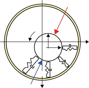
Figure 2.1 Bearing as part of a rotating system. Question marks indicate the places where dynamic coefficients of bearings occur. 15
Figure 2.2 Different bearing models: (a) oscillating mass with one degree of freedom; (b) bi-directional oscillating mass (two degrees of freedom); and (c) bi-directional oscillating mass with the inclusion of crosscoupled stiffness and damping coefficients. 16
Figure 2.3 Displacement of the mass attached to a fixed support by means of stiffness and damping coefficients as a result of a constant force. 18
Figure 2.4 The effect of a change in the damping coefficients on the displacement of the mass point which is being acted on by a constant force. The arrows represent the direction of displacement change due to the increase of damping coefficient values. 19
Figure 2.5 The effect of a change in the stiffness coefficients on the displacement of the mass point which is being acted on by a constant force. The arrows represent the direction of displacement change due to the decrease of stiffness coefficient values. 19
Figure 2.6 A single degree of freedom system with harmonic excitation. 20
Figure 2.7 The effect of a change in the damping coefficients on the displacement of the mass point which is being acted on by a constant harmonic with a frequency of 300 Hz. 21
Figure 2.8 The effect of a change in the stiffness coefficients on the displacement of the mass point which is being acted on by a constant harmonic with a frequency of 300 Hz. 22
Figure 2.9 Excitation force of constant value and of variable value changing along with frequency. 23
Figure 2.10 The relationship between the excitation force frequency and the amplitude of the system response for a constant force F. 23
Figure 2.11 The relationship between the excitation force frequency and the amplitude of the system response for the force F variable along with frequency. 24
Figure 2.12 Impact of damping coefficients. 25
Figure 2.13 Impact of stiffness coefficients. 25
Figure 2.14 Impact of mass coefficients. 26
Figure 2.15 Areas of influence of different types of coefficients for variable amplitude values of excitation force. 26
Figure 2.16 Areas of influence of different types of coefficients for the constant amplitude of excitation force. 27
Figure 2.17 Combination of oscillation in two directions taking into account the main stiffness and damping coefficients of the bearing 27
Figure 2.18 Two-directional displacement and trajectories: (a) cxx = cyy = 6400 N·s/m; (b) cxx·2; and (c) cyy·2. 29
Figure 2.19 Combination of oscillation in two directions taking into account the main and cross-coupled stiffness and damping coefficients of the bearing. 30
Figure 2.20 Trajectory changes: (a) cxy and cyx = 0 N·s/m; (b) cxy = 0 N·s/m and cyx = 6400 N·s/m; and (c) cxy = 0 N·s/m and cyx = 6400 N·s/m. 31
Figure 2.21 Trajectory changes: (a) kxy and kyx = 0 N/m; (b) kxy = 6 630 000 N/m and kyx = 0 N/m; and (c) kxy = 0 N/m and kyx = 6 630 000 N/m. 32
Figure 3.1 Photograph of the laboratory test rig. 35
Figure 3.2 Diagram of the laboratory test rig. 35
Figure 3.3 (a) Hydrodynamic bearing and (b) bearing diagram. 36
Figure 3.4 Run-up of the laboratory test rig; during 66.4 seconds the speed was increased linearly from 1000 to 8400 rpm. 37
Figure 3.5 Maximum displacement of the rotor journals. 37
Figure 3.6 Stable operation of bearings no. 1 (a and b) and no. 2 (c and d) at 3250 rpm; the diagrams show the signal recorded in X (a and c) and Y (b and d) directions; the short time interval (0.3 seconds) shows approximately 8 revolutions. 38
Figure 3.7 Stable operation of bearings no. 1 (a and b) and no. 2 (c and d) at 3250 rpm; the diagrams show the signal recorded in X (a and c) and Y (b and d) directions during 10 seconds. 39
Figure 3.8 FFT analysis of the stable operation signal from eddy current sensors bearings no 1 (a and b) and no 2 (c and d) at 3250 rpm; the diagrams show the signal measured in X (a and c) and Y (b and d) directions. 40
Figure 3.9 Trajectory of bearing journal movement no 2 during stable operation at a speed of 3250 rpm: (a) signal measured by sensors and (b) signal after filtering operation. 41
Figure 3.10 Combination of the vibration trajectories of a second bearing operating on a laboratory test rig for (a) below resonance speed (3250 rpm), (b) close to resonance speed (4500 rpm), and (c) above resonance speed (5750 rpm). 41
Figure 3.11 Cascade diagram based on the accelerometer signal placed on support no. 2 in the X direction (horizontal); on the drawing is highlighted the result of the FFT analysis at a rotational speed of 3000 rpm (dark gray horizontal line). 42
List of Figures
Figure 3.12 The first form of natural vibrations of the laboratory test rig. 44
Figure 4.1 SCADAS mobile analyzer. 47
Figure 4.2 (a) Eddy current sensors placed at a 90° angle to each other and perpendicular to the rotor axis and (b) module used for processing signals from eddy current sensors – demodulator. 47
Figure 4.3 (a) Accelerometer used to measure accelerations of vibrations of the bearing supports and (b) portable accelerometer calibrator. 48
Figure 4.4 Impact hammer 48
Figure 4.5 (a) Speed measurement using a laser sensor and (b) fiber optic switch. 48
Figure 4.6 The Vision Research Phantom v2512 camera (right), the LED lamps used for illumination (center), and the laboratory test rig (left). 49
Figure 4.7 (a) MBJ Diamond 401 measuring device used for balancing the rotor and (b) the OPTALIGN Smart RS device for shaft alignment. 50
Figure 4.8 Interface of the Test.Lab 11B software. 50
Figure 4.9 Interface of the Samcef Rotors software. 51
Figure 4.10 Interface of the Matlab software. 52
Figure 4.11 Interface of GRAFMESWIR – a graphical processor of the NLDW software. 53
Figure 4.12 Interface of the Abaqus/CAE software 6.14-2. 54
Figure 5.1 (a) Rotor model in the Samcef Rotors software and (b) bearing model. 56
Figure 5.2 Diagram for the calculation of dynamic bearing coefficients. 59
Figure 5.3 (a) Force in direction X as a function of time and (b) displacement of bearing no. 2 as a function of time. 61
Figure 5.4 (a) Frequency distribution of force and (b) amplitude of node no. 2 as a function of frequency. 61
Figure 5.5 Bearing no. 1: (a) flexibility amplitude and (b) flexibility phase. 61
Figure 5.6 The first form of natural vibrations of the rotor at 46 Hz. 62
Figure 6.1 Calculation scheme of dynamic coefficients of bearings including unbalance. 66
Figure 6.2 (a) Stable operation of the rotor – reference signal in the bearing and (b) amplitude of vibrations after inducing the rotor by means of a impact hammer – signal in the bearing 66
Figure 6.3 (a) Amplitude of vibrations after subtracting the reference signal from the excitation signal and (b) fast Fourier transform of this signal. 67
Figure 6.4 The fast Fourier transform displacement signal in bearings for rotational speed (a) 2800 rpm and (b) 10 000 rpm. 68
Figure 6.5 Dynamic flexibility of bearings: (a) amplitude course and (b) phase angle course. 68
Figure 7.1 Diagram showing the sensitivity analysis scheme. 71
Figure 7.2 (a) Rotor model on which the method of force displacement is marked. (b) Bearing response signal for the first bearing in the X direction after inducing the system in the X direction; comparison after excitation in the middle and force displaced by the value s = 30 mm. 73
Figure 7.3 (a) Model showing how the force is applied at an angle and (b) the response signal of the first bearing in the X and Y directions after excitation at an angle of α = 0° and α = 15°. 75
Figure 7.4 Model on which the place of bearing displacement measurement was marked (systems with p indexes) and places taken into account during calculation of dynamic coefficients of bearings (means of bearing housings). 77
Figure 7.5 Diagram of an asymmetrical rotor. 78
Figure 7.6 Response of an asymmetrical rotor system. 78
Figure 8.1 Program window for signal preparation; the diagrams presented the data read for a signal corresponding to a speed of 4500 rpm and excitation in the Y direction. 83
Figure 8.2 Window of the software used for calculations of dynamic coefficients of bearings. 84
Figure 8.3 Photograph showing the test stand during the shaft alignment. 86
Figure 8.4 Photograph showing the tested rotor. 86
Figure 8.5 Phantom Camera Control, a program window for operating a highspeed camera; a fragment of the recording of inducing the rotor with a impact hammer can be seen in the background. 87
Figure 8.6 Calculation scheme of dynamic coefficients of bearings. 88
Figure 8.7 Signal measured near bearing no. 2 in the Y direction at 4500 rpm and excitation with a impact hammer in the Y direction. 89
Figure 8.8 Excitation force curve in the Y direction over 20 seconds; signal stored at 4500 rpm. 89
Figure 8.9 Excitation force in the X and Y directions over 0.4 ms; excitation at 4500 rpm. (a) Values not reset outside the main peak and (b) signal with resetting. 90
Figure 8.10 Stable bearing operation no. 2 (a and b) at 4500 rpm and signal after excitation (c and d); the graphs show the displacements in the X direction (a and c) and Y direction (b and d); the time of the signal shown in the graphs is 0.1 seconds. 91
Figure 8.11 Amplitude of rotor vibrations after excitation in the X and Y directions for the first (a) and second (b) bearings; the reference signal has been subtracted from the signal after the excitation. 92
Figure 8.12 Changes in the stiffness coefficients of bearing no 2 for the entire speed range. 97
Figure 8.13 Changes in the damping coefficients of bearing no 2 for the entire speed range. 97
Figure 8.14 Changes in the mass coefficients of bearing no. 2 for the entire speed range. 97
Figure 8.15 Increasing vibration amplitude recorded in bearing no. 2 during operation at 4000 rpm after excitation with an impact hammer in the Y direction. 98
Figure 8.16 Schematic model of mass, damping, and stiffness. 99
List of Figures
Figure 8.17 Comparison of the dynamic response of the real rotor and the numerical model (the model takes into account the experimentally determined stiffness and damping coefficients). 99
Figure 9.1 Coordinate system at a selected point in the lubrication gap. 103
Figure 9.2 Algorithm of calculation of a radial hydrodynamic bearing 108
Figure 9.3 Numerical rotor model in the KINWIR program. 109
Figure 9.4 Numerical model of hydrodynamic bearing 110
Figure 9.5 Presentation of the pressure distribution calculated for the static equilibrium point at a speed of 3250 rpm in the Kinwir program. 110
Figure 9.6 Bearing no 2 stiffness coefficients calculated using a linear algorithm in the KINWIR program. 112
Figure 9.7 Bearing no 2 damping coefficients calculated using a linear algorithm in the KINWIR program. 112
Figure 9.8 Numerical model of the rotor, bearing and disk in the NLDW program. 113
Figure 9.9 Pressure distribution calculated using the NLDW program for (a–d) 4 journal positions (in 90° increments) at 3250 rpm. 114
Figure 9.10 Stiffness coefficients calculated in the NLDW program for 3 rotor revolutions at a rotational speed of 3250 rpm. 116
Figure 9.11 Damping coefficients calculated in the NLDW program for 3 rotor revolutions at a speed of 3250 rpm. 116
Figure 9.12 Stiffness coefficients calculated in the NLDW program for 3 rotor revolutions at a rotational speed of 3750 rpm. 117
Figure 9.13 Damping coefficients calculated in the NLDW program for 3 rotor revolutions at a speed of 3750 rpm. 117
Figure 9.14 Stiffness coefficients calculated in the NLDW program for 3 rotor revolutions at a rotational speed of 5500 rpm. 118
Figure 9.15 Damping coefficients calculated in the NLDW program for 3 rotor revolutions at a speed of 5500 rpm. 118
Figure 9.16 Bearing journal displacements calculated using the method with a linear calculation algorithm. 119
Figure 9.17 Bearing journal displacements calculated using the NLDW program. 120
Figure 9.18 Vibration trajectories of the journal of bearing no 2: (a) measured during experimental tests: (b) calculated using a linear algorithm: and (c) calculated using the NLDW program. 121
Figure 9.19 The FFT analysis of the signal for a speed of 5750 rpm based on experimental tests in the direction of (a) X and (b) Y; analogous results calculated numerically for the linear algorithm in the direction of (c) X and (d) Y; calculations by means of a non-linear algorithm in the NLDW program in the direction of (e) X and (f ) Y. 122
Figure 10.1 (a) Change in journal vibration trajectory due to e.g. increased rotor unbalance or changes in bearing parameters (trajectory 1, 2, or 3). (b)
Trajectory after inducing a bearing operating at a static equilibrium point (Oc). A model showing the assumptions of linear operation of the
List of Figures xv system. (c) Trajectory after excitation during operation with a larger ellipse of vibrations. The dotted line shows a sample trajectory after excitation in point Ow. After a short time, the rotor journal returns to the previous constant ellipse on which it was moving earlier (shown by a continuous line). 127
Figure 11.1 A diagram of the work carried out. The division into experimental tests and numerical analyses and the relationships between the various chapters and sections of the monograph are indicated. 130
Figure A.1 Fast Fourier transform (FFT) diagrams of the first and second bearings in the X and Y directions for rotational speeds of 2250–3000 rpm. 135
Figure A.2 FFT diagrams of the first and second bearings in the X and Y directions for rotational speeds of 3250–4000 rpm. 136
Figure A.3 FFT diagrams of the first and second bearings in the X and Y directions for rotational speeds of 4250–5000 rpm. 137
Figure A.4 FFT diagrams of the first and second bearings in the X and Y directions for rotational speeds of 5250–6000 rpm. 138
Figure A.5 Vibration trajectory of the first bearing for 16 rotational speeds, from 2250 to 6000 rpm. 139
Figure A.6 Vibration trajectory of the second bearing for 16 rotational speeds, from 2250 to 6000 rpm. 140
Figure A.7 Cascade diagram of an accelerometer placed on support no. 1 in the X direction (horizontal). 141
Figure A.8 Cascade diagram of an accelerometer placed on support no. 1 in the Y direction. 141
Figure A.9 Cascade diagram of an accelerometer placed on support no. 2 in the X direction. 142
Figure A.10 Cascade diagram of an accelerometer placed on support no. 2 in the Y direction. 142
Figure A.11 Shaft alignment report – part one. 143
Figure A.12 Shaft alignment report – part two. 144
Figure C.1 Vibration trajectories calculated for the second bearing using a linear algorithm based on the KINWIR and LDW programs. 153
Figure C.2 Vibration trajectories calculated for the second bearing using a nonlinear algorithm in the NLDW program. 154
List of Tables
Table 3.1 Successive eigenfrequencies and the corresponding damping values calculated for the laboratory test rig 43
Table 5.1 Parameters of the numerical model. 59
Table 5.2 Stiffness coefficients. 60
Table 5.3 Damping coefficients. 60
Table 5.4 Mass coefficients. 63
Table 7.1 Summary of the real and calculated stiffness, damping and mass coefficients for the two bearings for the reference case; representation of the relative calculations error. 72
Table 7.2 Summary of the real and calculated stiffness, damping, and mass coefficients for the two bearings for a case with displaced force; results “with correction” take into account the uneven distribution of excitation force in the calculation procedure. 74
Table 7.3 Summary of the real and calculated stiffness, damping and mass coefficients for the two bearings for a case with an excitation at an angle of α = 15°. 76
Table 7.4 Summary of the real and calculated stiffness, damping and mass coefficients of two bearings for an asymmetrical rotor. 78
Table 8.1 Stiffness, damping and mass coefficients of the rotor–bearing system for the entire speed range. 95
Table 8.2 Standard deviation of stiffness, damping and mass coefficients of the rotor – bearing system for the entire speed range. 96
Table 9.1 Parameters of the numerical model in the KINWIR program. 109
Table 9.2 Stiffness and damping coefficients obtained from linear calculations in the KINWIR. 111
Table 9.3 Minimum and maximum values of stiffness coefficients (N/m) calculated in the NLDW program. 115
Table 9.4 Minimum and maximum values of damping coefficients (N·s/m) calculated in the NLDW program. 115
Table 10.1 Comparison of the calculated stiffness and damping coefficients for the three methods used for a speed of 3000 rpm. 126
Preface
This monograph concerns the experimental and numerical methods of determination of dynamic coefficients of hydrodynamic radial bearings. Bearings are one of the basic elements influencing the dynamics of rotor machinery. The main parameters with which the operation of bearings can be described (and thus the operation of the entire rotating system) are their stiffness and damping coefficients.
This book includes a chapter about practical applications of bearing dynamic coefficients. It is shown how changes of bearing dynamic coefficients affect the dynamic performance of rotating machinery. Some examples are included with all the necessary data to allow rotordynamics analysis to be conducted and the dynamic coefficients of journal bearings to be calculated so that the readers can replicate the results presented in this book and compare them with their own results. This book presents in detail an experimental method of determining dynamic coefficients of bearings. An additional objective is to describe numerical methods of determining dynamic coefficients of hydrodynamic bearings (linear and non-linear). The range of applicability of various calculation methods was determined based on measurements made for a rotating machine equipped with hydrodynamic bearings with clearly non-linear operating characteristics.
Experimental research was carried out with the use of the impulse method, on the basis of which dynamic parameters of hydrodynamic bearings were determined. The applied method with a linear calculation algorithm allows the determination of stiffness and damping coefficients and the determination of mass coefficients in one algorithm. The stiffness and damping coefficients cannot be determined directly, thus indirect calculation methods are used. The mass of the rotor is a directly measurable parameter. Indirectly calculated mass coefficients can be compared with the known mass of the rotor. On this basis, it is possible to make preliminary estimations of the correctness of the results obtained.
As part of the study, the sensitivity analysis of the aforementioned experimental method was carried out with the use of a model created in Samcef Rotors software. The influence of unbalance, displacement of measuring sensors, and various variants of driving force were analyzed. Based on experimental research, dynamic coefficients of hydrodynamic bearings in a wide range of rotational speeds, taking into account resonance speeds and higher speeds, were determined. They were verified using Abaqus software.
Numerical calculations of stiffness and damping coefficients of hydrodynamic bearings with the use of linear and non-linear calculation models developed by IMP PAN in Gdańsk were also carried out. The obtained results were verified. The stiffness and damping
Preface xviii
parameters of hydrodynamic bearings determined using numerical models (linear and non-linear) were compared with the results of experimental research. From this comparison it was possible to evaluate the differences in the values of dynamic coefficients of bearings calculated on the basis of linear and non-linear numerical methods and the experimental method.
I would like to thank all employees of the Turbine Dynamics and Diagnostics Department of the Polish Academy of Sciences for their kindness, for the atmosphere of friendship that they surrounded me with throughout the entire period of work, and for the fact that I could always count on their support and research experience. In particular, I would like to express my gratitude to Professor Grzegorz Żywica and Professor Jan Kiciński.
Gdańsk, November 2020 Łukasz Breńkacz
Symbols and Abbreviations
Symbols
βi,k dimensionless damping coefficients of lubricating film, i,k = x,y
γi,k dimensionless stiffness coefficients of lubricating film, i,k = x,y
μ dynamic viscosity of oil, N·s/m2 = Pa·s
μo oil viscosity at temperature T0, N·s/m2 = Pa·s
Π dimensionless hydrodynamic pressure, Π = p(ΔR/R)2/μ0Ω
Π* pressure at static equilibrium point
σ standard deviation
τ dimensionless time τ = ωt
ψ angular coordinate x R , rad, angles defining position of outlet and inlet edges of lubricating pockets
ω frequency, rad/s, rotational speed, rpm
Ω journal angular velocity, rad/s
Abbreviations
A integral values according to Eq. (9.2)
B integral values according to Eq. (9.2)
c damping
csij damping coefficients of bearing no. s, N·s/m, s = 1,2; i,j = x,y
d shaft and bearing journal diameter, m
D disk diameter, m
Dz bearing housing diameter, m
Dsij displacement of bearing no. s in the frequency domain, m, s = 1,2; i,j = x,y
FNi force in the N direction, N = x,y
Fsi,j flexibility vector of bearing no. s, m/N, s = 1,2; i,j = x,y
F1, F2 functions describing dynamic coefficients of bearings
Hsi,j stiffness vector of bearing no. s, N/m, s = 1,2; i,j = x,y
h lubrication gap thickness, m
Symbols and Abbreviations xx
H dimensionless thickness of lubrication gap, H = h/ΔR
k stiffness
ksij stiffness coefficients of bearing no. s, N/m, s = 1,2; i,j = x,y
L bearing housing width, m
m mass
msij mass coefficients of bearing no s, kg, s = 1,2; i,j = x,y
Oc center of bearing journal
Op center of the coordinate system associated with the bearing housing P0 force acting on the bearing
p hydrodynamic pressure in the lubricating film, Pa
R journal radius, m
ΔR radial bearing backlash, m
S0 Sommerfeld number (dimensionless load-bearing capacity of bearings),
S0 = Pst(ΔR/R)2/LDμ0Ω
t time, s
u, v, w speed components of the liquid element in the coordinate system x, y, z, m/s
U1, V1, W1 components of lower sliding surface speed, m/s
U2, V2, W2 components of upper sliding surface speed, m/s
Wx, Wy dynamic components of the reaction of lubricating film, N
ΔWx, ΔWy changes in the dynamic components of the reactions of lubricating film, N
W0 static components (at equilibrium point) of the reactions of lubricating film, N
x̅ mean value
x,y,z coordinates
Xc,Yc,Zc rectangular coordinate system related to the position of the journal center (Oc)st at the static equilibrium point, m
Xp,Yp,Zp rectangular coordinate system related to the bearing housing center Op, m
Xc,Yc,Zc dimensionless rectangular coordinate system related to the position of the journal center (Oc)st at the static equilibrium point (Xc = xc/ΔR)
X c , Yc disturbing parameters
Z matrix of dynamic coefficients of bearings
The book is accompanied by a companion website: www.wiley.com/go/brenkacz/bearingdynamiccoefficients
The website includes:
● Computational codes
● Recordings
Introduction
The analysis of dynamic properties of rotating machinery has for many years been the subject of numerous research studies carried out in many scientific centers. For modern day rotating machinery it is required to work with increasingly difficult operating parameters while maintaining a light and compact design. Increased efficiency, reliability, and precision are also required. Rotating machinery with hydrodynamic bearings is used in many sectors of the economy, e.g. energy, transport, aviation, and military. Very often they are a key element of large technical objects.
In steam turbines used for energy conversion, one of the key components are hydrodynamic plain bearings. These machines are referred to as “critical machinery,” i.e. they are required to be extremely reliable. Unplanned downtime due to poor technical condition leads to significant financial losses. They are therefore monitored and thoroughly analyzed.
The starting point for the analysis of hydrodynamic radial bearings are the equations of motion. From the mathematical perspective, we are dealing with non-linear differential equations (motion equations of the entire rotor) related to the system of partial differential equations describing the properties of plain bearings and the supporting structure. This association occurs through the stiffness and damping coefficients of hydrodynamic bearings. These coefficients determine the dynamic properties of the bearings. Linear and nonlinear numerical calculation models are available, but the limit from which the much more complex and time-consuming non-linear models must be used is not clearly defined. An experimental (using a linear algorithm) and numerical (using linear and non-linear algorithms) calculation of dynamic coefficients of bearings for a wide range of rotational speeds was carried out in order to elaborate on the issue formulated in the title of this monograph.
1.1 Current State of Knowledge
The values of stiffness and damping coefficients have a decisive impact on the analysis of rotary machine vibrations. During the dynamic analysis of the rotating shaft, it is necessary to build a discrete model, define the boundary conditions, and calculate the values of these coefficients. The stiffness and damping coefficients change with rotational speed. For the majority of bearings in operation, the coefficients are non-linear in nature,
Bearing Dynamic Coefficients in Rotordynamics: Computation Methods and Practical Applications, First Edition. Łukasz Breńkacz.
© 2021 John Wiley & Sons Ltd. This Work is a co-publication between John Wiley & Sons Ltd and ASME Press. Companion website: www.wiley.com/go/brenkacz/bearingdynamiccoefficients
which means that they change in time and are dependent on the driving force (Kiciński 2006). For most jobs, a linearized form of coefficients is used, which means that they have constant values for a given speed and do not change for different values of driving forces. It should be remembered that dynamic coefficients also change with changes in operating temperature, bearing supply pressure, and bearing load (Hamrock et al. 2004).
For many years at the Institute of Fluid Flow Machinery in Gdańsk under the management of Professor Jan Kiciński, programs from the MESWIR series for numerical calculation of dynamic coefficients of hydrodynamic bearings and rotor dynamics together with imperfections have been developed. A key element in the calculation is the appropriate determination of the stiffness and damping coefficients of hydrodynamic bearings. In the NLDW software (one of the programs of the MESWIR series) it is possible to determine the non-linear form of these coefficients. This is the basis for further dynamic analysis of the entire system, which can be conducted on many planes. Unfortunately, only an indirect comparison of the results of numerical calculations with a real model is possible, i.e. by comparing the amplitudes of vibrations measured on the basis of experimental tests and the amplitudes of vibrations calculated on the basis of numerical analyses. This work presents a method which enables dynamic coefficients of bearings to be determined on the basis of experimental research. They can be directly compared with the results of numerical tests.
Numerical determination of stiffness and damping coefficients of bearings is most often performed by solving the Reynolds differential equation. For linear systems with known parameters such calculations are performed with very high accuracy (Duff and Curreri 1960; Giergiel 1990). For systems for which it is necessary to describe using methods with non-linear calculation algorithms (Hayashi 1964), or methods with complex structure with unknown parameters, calculations become more complicated and are often plagued with significant errors (Fertis 2010). During the calculation it is necessary to take into account the relationships between different parts of the system such as rotor, bearings, and supporting structure (Kiciński and Żywica 2014a; Mikielewicz et al. 2005).
The principles of hydrodynamic lubrication of bearings and the principles of formation of a wedge of lubricant are described in many books on the theory and practice of plain bearings (Neyman and Sikora 1999; Wierzcholski 1994). Numerical linear and non-linear algorithms for calculating stiffness and damping coefficients of hydrodynamic radial bearings are presented in an accessible way in the book Teoria i badania hydrodynamicznych poprzecznych łożysk ślizgowych (Theory and Research on Hydrodynamic Radial Plain Bearings) (Kiciński 1994). The hydrodynamic bearing can be treated as a mechanical system consisting of elements of varied stiffness. The properties of the bearing are determined by the lubricating film that forms between the journal and the bearing housing (Sikora 2009). Bearing properties are defined as the properties of a lubricating film.
A schematic view of a hydrodynamic radial bearing is shown in Figure 1.1. In the center of the bearing housing there is a rectangular system of coordinates Xp, Yp with the center marked as Op. Under conditions of static equilibrium a relationship occurs (1.1), where W0 is the reaction of the lubricating film to the force P0, while Xp, Yp, Yp determine the position of the center of the journal Oc.
It is important to note that the f(xp, yp) function, which determines the relationship between the reaction of the film and the displacement of the journal, is non-linear, and this non-linearity increases strongly with the increase of displacements of xp, yp. The reaction W0 can be written as the sum of the reactions Wx and Wy in two perpendicular directions. Definition of the stiffness coefficients of the lubricating film are determined by Eqs. (1.2) and (1.3):
where ΔWx, ΔWy are the changes in the reaction of the film due to a small increase in force ΔP at the point of static equilibrium, and Δx, Δy are the changes in journal displacements due to an increase in force ΔP calculated at the point of static equilibrium. A characteristic feature of radial plain bearings is their inequality of “cross-coupled” reaction and displacement ratios, i.e. inequality of coefficients kxy kyx. This is not a property of linear-elastic mechanical systems. It turns out that it is the cause of hydrodynamic instability.
The stiffness of the lubricating film, as an analogy of mechanical systems, often assumes that xp, yp displacements are slow. However, in hydrodynamic bearings, when the journal performs small, fast oscillations around the static equilibrium point, significant additional components of the Wx and Wy reaction may arise due to the resistance to motion in the viscous lubricant. In addition to the elastic properties, it is also necessary to determine the damping properties of the lubricating film. They can be formulated using Eqs. (1.4) and (1.5) in the same way as for the stiffness coefficients:
Figure 1.1 Lubrication film model for small journal displacement.
where xc , yc mean the derivative of the displacement in time.
In numerical calculations, the following relationship is used, i.e. in case of damping there is no anisotropy of “cross-coupled” coefficients, i.e. cxy = cyx (Kiciński 1994). Assuming small displacements xc, yc, elastic and damping properties of the lubricating film can be described by four stiffness coefficients and four damping coefficients. In numerical analyses three damping coefficients can be obtained. The components of the reaction of the lubricating film – Wx, Wy – can be represented by linear relationships (1.6) and (1.7):
The dynamic components Wx,Wy depend on the momentary position of the center of the journal xc, yc. Assuming that kxx, kxy, kyx, kyy = ki,k and cxx, cxy, cyx, cyy = ci,k these coefficients can be described by Eq. (1.8), where the functions F1 and F2 are non-linear. Wx and Wy relationships form the basis for a linear description of dynamic properties of the lubricating film and rotor–bearing systems (Dąbrowski 2013). They can be used to quickly and easily determine a number of very important characteristics of hydrodynamic bearings. Due to the non-linear nature of bearings, a linear description can only reflect the actual bearing properties and the system associated with them to a limited extent. In this monograph the results of calculations using linear algorithms are shown on a specific example of a laboratory test rig operating with parameters which should be described using methods with non-linear algorithms.
The non-linear description is much more complicated than the linear one (Batko et al. 2008; Minorsky 1967; Skup 2010), but it allows (by determining the trajectory of the journal) to analyze e.g. self-excited vibrations of the system or to determine the influence of various types of external forces and damage. It provides much greater opportunities for theoretical analysis of the bearing’s operation and the system associated with it. However, its use may be limited by the time of numerical calculations and computing capabilities of computers. As the computing power of computers increases, these limitations become less and less significant.
The methods most frequently used in non-linear analysis consist of the use of non-linear equations of motion and the principle of superposition to solve the Reynolds equation, where at each time point the part of the equation referring to the so-called combined effect of the rotational speed of the journal (the “kinetostatic” part) and to the so-called extrusion effect (the “dynamic” part) is solved separately. The above principle is the basis for the vast
1.1 Cuurent nttntr of e owredr 5
majority of numerical methods of determining the trajectory of a journal in the case of large displacement, e.g. methods developed by Booker, Block, and other authors (Blok 1975; Booker 1965). They have one common flaw, i.e. when the solutions are compiled different boundary conditions are used in the “kinetostatic” part and in the “dynamic” part of the Reynolds equation (Kiciński 1994).
It is possible to formulate a non-linear description without the above-mentioned flaw (Kiciński 1994). This description can be based on four predefined stiffness coefficients and four damping coefficients and is used in the MESWIR environment. If the whole interval of variation of the journal trajectory is divided into a sufficiently large number of successive subintervals at small intervals of Δt, it may be assumed that there are areas of the circle of backlash corresponding to those subintervals in which the stiffness and damping coefficients are approximately constant. Each such area will have constant coefficients which need to be determined. The characteristic feature of this method of determining the stiffness and damping coefficients is the fact that for each such area the full Reynolds equation is solved with only one boundary conditions (and thus without the use of superposition solutions). The dynamic components Wx,Wy depend not only on the momentary position of the center of the journal xc, yc, but also on the speed of change of this position xc , yc , according to Eq. (1.9) (Buchacz et al. 2013).
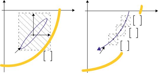
The functions F1 and F2 are non-linear, as in the case of small vibrations around the static equilibrium point. Based on the above at each time point of the trajectory tk−1, tk, tk+1, etc., and based on the determined stiffness and damping coefficients, it is possible to determine the increments of displacement Δx and Δy in a stepwise procedure. The accuracy of the calculation will increase as the time step decreases, i.e. as the areas in which the stiffness and damping coefficients can be assumed to be constant decrease. This relationship will be true until a certain point, and with too small time steps the accuracy of the calculations will be limited. Figure 1.2 illustrates the difference between linear and non-linear analysis based on stiffness and damping coefficients. The hatched fields show the areas where the coefficients are approximately constant.
The numerical analysis of vibrations with regard to large displacements of the journal carried out with the methods discussed above, regardless of whether it uses the principle of superposition or not, which is described as non-linear, is in fact a linear analysis of “pseudostatic” states (Kiciński 1994). In this context, bearing dynamics is a sum of separate “pseudostatic” states, in which time is treated as a parameter. In practice, the state of the bearing at any time tk is influenced by phenomena occurring at moments preceding the moment under consideration, i.e. tk−1, tk−2, etc. This means that it is necessary to “memorize” the entire history of previous states and a continuous mathematical description in which time is no longer a parameter but is the third (next to geometric coordinates) independent variable.
In the case of a description with “prehistory”, the time relationships used ensure that the Reynolds equation will not be integrated in an “empty” lubrication gap. In the MESWIR environment, where numerical analyses were performed, a continuous description with “prehistory” is used.
(a)
Linear analysis
(b)Non-linear analysis
Trajectory of the journal center
Bearing housing
Trajectory of the journal center
Bearing housing
Figure 1.2 Methods of analysis for (a) small and (b) large displacement of the journal.
1.2 Review of the Literature on Numerical Determination of Dynamic Coefficients of Bearings
Attempts at a theoretical description of the operation of rotating machinery have been undertaken since objects with rotating elements began to be used in practice (Chmielniak 1997; Miller 1985; Zieliński 1969). The intensive development of these machines, and with it a more detailed description of them, took place at the turn of the eighteenth and nineteenth century. Significant progress in the theoretical description of rotating machinery began with pioneering works on turbines used for energy conversion (Bannik and Słuczajew 1956; Chodkiewicz 1998; Kiciński and Żywica 2014b; Łączkowski 1974; Nikiel 1956; Smolaga 1959; Wiśniewski 1974). The basis for the theoretical model of hydrodynamic plain bearings is the fundamental equation of hydrodynamic lubrication theory, i.e. Reynolds equation (Reynolds 1886). To this day we encounter some problems, the most important of which are (Barwell 1984): analysis of three-dimensional flow in the bearing lubrication gap, taking into account changes in viscosity, and determining the limits of integration of the pressure distribution curve (which is related to the occurrence of cavitation phenomenon). The impact of the supporting structure (Żywica 2008) is not insignificant either.
The first researcher who suggested applying Reynolds’ theory to the calculation of slide bearing dynamics was S. Dunkerley in 1894 (Dunkerley 1894). In 1904 Sommerfeld solved the case of two-dimensional flow in plain bearings on the assumption that the liquid is able to transfer an unlimitedly high pressure (Sommerfeld 1904). Such a simplification caused the obtained result to be incorrect, but a dimensionless parameter determining the hydrodynamic similarity of bearings, the so-called Sommerfeld number, was described. D.G. Christopherson was the first to solve the Reynolds equation using the relaxation method (Christopherson 1941). In his work he stated that assuming that viscosity of oil is constant, it is possible to correctly determine the value of the bearing’s load, the amount of oil flowing through the bearing, and temperature changes. The assumption made it
1.3 revro ofnttr vntrutntCur ef Exruvirenttw rntruivetntv e of Detivic roovicvrentts of rtuvedts 7
impossible to determine the exact friction resistance and load direction. This method (with the application of finite differences) was implemented by C. Cryer in 1971 (Cryer 1971).
H.W. Swift (1932) and W. Stieber (1933) proposed a method of modeling cavitation by applying boundary conditions, currently called Reynolds boundary conditions in the literature. The study of hydrodynamic instability was carried out by, among others, A.C. Hagg and P.C. Warner, who proved that the cause of this phenomenon is oil whirls (Hagg and Warner 1953). Even the most complex bearing models enabled the analysis of the rotor–bearing system only in the range of small vibrations. It is a linearization of systems, which in reality often showed strong non-linear properties. A typical approach is to assume constant values for the stiffness and damping coefficients of the lubricating film, which are determined only for the kinetostatic equilibrium point.
A more detailed examination of the properties of hydrodynamic bearings was made possible with the use of numerical calculation methods. The most commonly used methods are the finite volume method and the finite difference method (Lund 1987; Someya 1989; Wasilczuk 2012; Zienkiewicz and Taylor 2000). The finite element method is most frequently used to analyze the bearing journal displacement (Andreau et al. 2007).
While discussing the development of contemporary computational models, one should mention the considerable achievements of the Turbine Dynamics and Diagnostics Department (formerly the Department of Dynamics of Rotors and Slide Bearings), which is a part of the organizational structure of the Institute of Fluid Flow Machinery of the Polish Academy of Sciences in Gdansk. Under the management of Professor Jan Kiciński, new computational models of plain bearings have been developed and experimental research has been carried out for many years (Kiciński 1994, 1988; Kiciński et al. 1997). It is worth mentioning achievements such as the formulation of a non-linear elastodiatermic model of a plain bearing (Kiciński 1989) and participation in the development of the DT-200 diagnostic system. It was installed on one of the units of the power plant in Kozienice. Also a software package called MESWIR was created. It enables an extensive analysis of bearings and complex rotor lines, even after exceeding the stability limit. The MESWIR package includes, among others, the following programs: NLDW, KINWIR, LDW, TRADYN, DIADEF, ADIAB, ISOSLEW, and DYNWIR. The first three programs were also used during the numerical analysis presented in this monograph. The description of the MESWIR system can be found in Kiciński (2005).
In recent years, numerous attempts have been made to calculate stiffness and damping coefficients in various bearing configurations, for various lubricants (Zhang et al. 2015) and geometries (Illner et al. 2015). New types of bearings and their better numerical description are being developed. The impact of boundary cavitation conditions on dynamic systems with hydrodynamic bearings is described in Daniel et al. (2016). Characteristics describing the operation of a floating ring bearing are presented in Chasalevris (2016).
1.3 Review of the Literature on Experimental Determination of Dynamic Coefficients of Bearings
Due to difficulties in numerical calculation of stiffness and damping coefficients of bearings, many experimental methods have been proposed to determine these coefficients (Dimond et al. 2009; Tiwari et al. 2004). The calculation of stiffness and damping coefficients
can be performed in the time or frequency domain. Zhang et al. (1992a, 1992b) as well as Chan and White (1991) determined the stiffness and damping coefficients of two symmetrical bearings by adjusting the curves in the frequency response. This approach assumes a rotor with two identical bearings and allows for the calculation of eight dynamic factors (four stiffness coefficients and four damping coefficients). Since many rotor–bearing systems are not symmetrical and their vibration trajectories have more complex shapes than those for symmetrical systems, the limitation associated with the symmetry of the system in many cases cannot be applied. The method of curve matching also consumes a lot of computational power.
The work of Qiu and Tieu (1997) presents a method extending the calculation of eight coefficients of one bearing, allowing the calculation of a total of 16 stiffness and damping coefficients, for two different hydrodynamic bearings (four stiffness coefficients and four damping coefficients for each bearing). A method of determining the linearized form of coefficients (each stiffness and damping coefficient described by means of a single value) was developed. The authors believe that this method is the most effective method for determining stiffness and damping coefficients. In order to experimentally determine the stiffness and damping coefficients of bearings, it is necessary to force the rotor vibrations. This can be achieved in several ways. The three most commonly used are: impulse excitation of the rotating rotor by means of a modal hammer, the use of additional unbalance of the rotor, and the use of vibration inductors. Qiu and Tieu state in their work that the impulse excitation method is the most economical and convenient way to determine these coefficients. Dynamic coefficients of bearings are calculated on the basis of the response signal of the system measured after inducing the rotor in its central part by means of a modal hammer. The signals in the frequency domain are then used for further calculations. The authors suggest that a wider range of identification should be covered in the calculations in order to ensure greater repeatability of the results.
Tiwari and Chakravarthy (2009) described and demonstrated two different identification algorithms for the simultaneous estimation of the residual unbalance and the dynamic parameters of bearings of a rigid rotor–bearing system. The first method uses the impulse response measurements of the journal from bearing housings in the horizontal and vertical directions, for two independent impulses on the rotor in these directions. Time-domain signals of impulse forces and displacement responses are transformed into the frequency domain and are used for the estimation of the residual unbalance and bearing dynamic parameters. The second method employs the unbalance responses from three different unbalance configurations for the estimation of these parameters. The simulated responses were in fairly good agreement with experimental responses in terms of mimicking predominant resonances. The identified unbalance masses matched quite well with the residual masses taken in the dynamically balanced rotor–bearing test rig.
Meruane and Pascual (2008) described a method of numerical determination of nonlinear stiffness and damping factors of hydrodynamic bearings. The calculation of fluid film coefficients using a non-linear method was performed for large displacements in the bearing (20–60% of the bearing gap). The non-linear effect was defined by extending the third-order Taylor equations. The non-linear model was created on the basis of a laboratory test stand. It was found that non-linear properties were revealed with oil vortexes that are not taken into account in classical linear models.
1.3 revro ofnttr vntrutntCur ef Exruvirenttw rntruivetntv e of Detivic roovicvrentts of rtuvedts 9
Work on modification of experimental methods in order to obtain greater accuracy is currently in progress. Miller and Howard (2009) described a method for identifying stiffness and damping coefficients by using the extended Kalman filter. This filter was developed to estimate the linearized form of stiffness and damping coefficients of bearings in rotor–bearing systems, taking into account noise and unbalance. The system uses impulse excitation. In this method, bearings are modeled as stochastic, random values using the Gauss–Markov model. The noise part is introduced into the system as an estimation error, including modeling and uncertainty of measurement. The system contains two userdefined parameters that can be used to fine tune the operation of the filter. They refer to the covariance of the system and the noise variables. The filter was tested using numerically created data of a system of two identical bearings, reducing the number of unknown coefficients to eight. The method was used to determine the main dynamic coefficients of bearings, while the cross-coupled coefficients were determined with a lower accuracy.
Particular difficulties in numerical determination of dynamic coefficients of bearings may be caused by bearings of complicated construction, e.g. foil bearings (Kiciński and Żywica 2012). The results of experimental identification of dynamic coefficients of a large foil bearing are presented in Wang and Kim (2013). Dynamic characteristics of a hybrid foil bearing (hydrodynamic + hydrostatic), 101.6 mm in diameter and 82.6 mm in length, are presented in that work. The stiffness coefficients were determined using two methods: the quasi-static method by determining deflection curves in the time domain and the impulse method in the frequency domain. The values of damping coefficients were determined using the impulse method only. The values of stiffness coefficients determined using the two above methods were similar, with the differences of around 4–7 MN/m depending on the speed, load, and supply pressure. Frequency calculations were characterized by greater discrepancies in the obtained results. As part of the work, a numerical model was also created, using the linear perturbation method. On the basis of the shaft deflection it was found that the results were similar to those of the experimental research.
A paper by Delgado (2015) presents calculations for a hybrid gas bearing (Kazimierski and Krysiński 1981) of a complex construction, characterized by rigid geometry and complex foil construction. The bearing operates on two lubrication films: hydrostatic and hydrodynamic. Such a procedure ensures the generation of appropriate load-bearing capacity and stiffness of the entire system. The paper presents an experimental verification of stiffness and damping coefficients for a bearing with a diameter of 110 mm. The results were obtained on a specially designed laboratory test rig. The variable parameters during the experiment were: hydrostatic supply pressure, driving force frequency, and rotor speed. Experimental research was aimed at evaluating the application of this bearing type in large-scale energy conversion machines. The dynamic tests showed poor sensitivity of the main stiffness coefficients to most of the test parameters. The frequencies and speeds were an exception: the higher the speed and frequency of the driving force, the lower the value of the calculated stiffness coefficients.
A paper by Kozánek et al. (2009) presents the results of experimental calculations of aerostatic radial bearings on the Bentley Nevada laboratory test rig. Various types of bearings as well as their static and dynamic characteristics were examined. Different methods of identification of dynamic coefficients of bearings were applied. Only the main stiffness and damping coefficients were calculated. The impact of cross-coupled stiffness and damping parameters was examined on the basis of numerical simulations.
During calculations, the mass matrix was defined as a matrix of known parameters, stiffness and damping matrices were determined. The authors recommended that when conducting experimental research the main values of stiffness and damping coefficients should be determined first, followed by cross-coupled ones, which are more susceptible to errors. According to the authors, increasing the bearing supply pressure and frequency of driving force negatively affects the correctness of the obtained values of dynamic coefficients of bearings.
Another example of experimental determination of parameters of aerostatic bearings is presented in Kozánek and Půst (2011). As part of the paper, a numerical model was developed to calculate the stiffness and damping parameters of both radial and thrust bearings.
A new method of identification of stiffness and damping of a bearing, based on phase plane diagrams, is presented in a paper by Jáuregui et al. (2012). The authors emphasize that reliable determination of dynamic coefficients of bearings is a huge challenge, particularly in non-linear systems. They also claim that a single, universal mathematical model does not exist, and the identification of parameters of a system depends on the measured data and the reference model. This model of phase plane diagrams works well when the coefficients are strongly dependent on frequency.
Experimental calculations of stiffness and damping parameters of bearings are not only done for radial bearings, but also for thrust bearings. The experimental determination of the parameters of stiffness and axial damping of foil bearings are presented in a paper by Arora et al. (2011). The paper presents a diagram of the procedure of identification of these coefficients, a description of the laboratory test rig, and a diagram of the values of stiffness coefficients in the function of rotational speed. The Monte Carlo algorithm was used to determine the dynamic parameters of the rotor supported on the magnetorheological layer of the lubricating film (Zapomel et al. 2014).
The method of impulse excitation for the determination of bearing coefficients, which is used in this monograph, is carried out in the frequency domain. Its first basic version was proposed by Nordmann and Schoelhorn (1980). Qiu and Tieu extended the calculation algorithm with the possibility of calculating 16 stiffness and damping coefficients (Qiu and Tieu 1997). This monograph describes a modification of the algorithm developed by Qiu and Tieu to calculate the damping coefficients and stiffness of bearings (using the impulse method and approximation with the least squares method). The algorithm has been extended by the possibility of calculating eight mass coefficients. Determination of damping, stiffness and mass coefficients using a single algorithm enables verification of the results at the initial stage of operation. Since the mass of the shaft is usually a known size, the correctness of the determined dynamic coefficients of bearings can be verified on the basis of mass coefficients. This approach makes it possible to determine all dynamic parameters of the rotor–bearing system through experimental research.
1.4 Purpose and Scope of the Work
The analysis of the literature and research conducted earlier in the Institute of Fluid Flow Machinery of the Polish Academy of Sciences confirm that dynamic coefficients of bearings have a key influence on the dynamic properties of rotating machinery. Since experimental methods for determining the stiffness and damping coefficients of bearings are usually