FUNDAMENTALS OF PHYSICS
VICE PRESIDENT AND GENERAL MANAGER Aurora Martinez
SENIOR EDITOR John LaVacca
SENIOR EDITOR Jennifer Yee
ASSISTANT EDITOR Georgia Larsen
EDITORIAL ASSISTANT Samantha Hart
MANAGING EDITOR Mary Donovan
MARKETING MANAGER Sean Willey
SENIOR MANAGER, COURSE DEVELOPMENT AND PRODUCTION Svetlana Barskaya
SENIOR COURSE PRODUCTION OPERATIONS SPECIALIST Patricia Gutierrez
SENIOR COURSE CONTENT DEVELOPER Kimberly Eskin
COURSE CONTENT DEVELOPER Corrina Santos
COVER DESIGNER Jon Boylan
COPYEDITOR Helen Walden
PROOFREADER Donna Mulder
COVER IMAGE ©ERIC HELLER/Science Source
This book was typeset in Times Ten LT Std Roman 10/12 at Lumina Datamatics.
Founded in 1807, John Wiley & Sons, Inc. has been a valued source of knowledge and understanding for more than 200 years, helping people around the world meet their needs and fulfill their aspirations. Our company is built on a foundation of principles that include responsibility to the communities we serve and where we live and work. In 2008, we launched a Corporate Citizenship Initiative, a global effort to address the environmental, social, economic, and ethical challenges we face in our business. Among the issues we are addressing are carbon impact, paper specifications and procurement, ethical conduct within our business and among our vendors, and community and charitable support. For more information, please visit our website: www.wiley.com/go/citizenship.
Copyright © 2022, 2014, 2011, 2008, 2005 John Wiley & Sons, Inc. All rights reserved. No part of this publication may be reproduced, stored in a retrieval system or transmitted in any form or by any means, electronic, mechanical, photocopying, recording, scanning or otherwise, except as permitted under Sections 107 or 108 of the 1976 United States Copyright Act, without either the prior written permission of the Publisher, or authorization through payment of the appropriate per-copy fee to the Copyright Clearance Center, Inc., 222 Rosewood Drive, Danvers, MA 01923, website www.copyright.com. Requests to the Publisher for permission should be addressed to the Permissions Department, John Wiley & Sons, Inc., 111 River Street, Hoboken, NJ 07030-5774, (201) 748-6011, fax (201) 748-6008, or online at http://www.wiley.com/go/permissions.
Evaluation copies are provided to qualified academics and professionals for review purposes only, for use in their courses during the next academic year. These copies are licensed and may not be sold or transferred to a third party. Upon completion of the review period, please return the evaluation copy to Wiley. Return instructions and a free of charge return shipping label are available at www.wiley.com/go/returnlabel. Outside of the United States, please contact your local representative.
Volume 1: 9781119801191
Extended: 9781119773511 Vol 1 epub: 9781119801153 Vol 1 ePDF: 9781119801160
The inside back cover will contain printing identification and country of origin if omitted from this page. In addition, if the ISBN on the back cover differs from the ISBN on this page, the one on the back cover is correct.
Printed in the United States of America 10 9 8 7 6 5 4 3 2 1
1 Measurement 1
1.1 MEASURING THINGS, INCLUDING LENGTHS 1
What Is Physics? 1
Measuring Things 1
The International System of Units 2
Changing Units 3
Length 3
Significant Figures and Decimal Places 4
1.2 TIME 5
Time 5
1.3 MASS 6
Mass 7
REVIEW & SUMMARY 8 PROBLEMS 8
2 Motion Along a Straight Line 13
2.1 POSITION, DISPLACEMENT, AND AVERAGE VELOCITY 13
What Is Physics? 13
Motion 14
Position and Displacement 14
Average Velocity and Average Speed 15
2.2 INSTANTANEOUS VELOCITY AND SPEED 18
Instantaneous Velocity and Speed 18
2.3 ACCELERATION 20
Acceleration 20
2.4 CONSTANT ACCELERATION 23
Constant Acceleration: A Special Case 23
Another Look at Constant Acceleration 27
2.5 FREE-FALL ACCELERATION 28
Free-Fall Acceleration 28
2.6 GRAPHICAL INTEGRATION IN MOTION ANALYSIS 30
Graphical Integration in Motion Analysis 30
REVIEW & SUMMARY 32 QUESTIONS 32 PROBLEMS 33
3 Vectors 44
3.1 VECTORS AND THEIR COMPONENTS 44
What Is Physics? 44
Vectors and Scalars 44
Adding Vectors Geometrically 45
Components of Vectors 46
3.2 UNIT VECTORS, ADDING VECTORS BY COMPONENTS 50
Unit Vectors 50
Adding Vectors by Components 50 Vectors and the Laws of Physics 51
3.3 MULTIPLYING VECTORS 52
Multiplying Vectors 53
REVIEW & SUMMARY 58 QUESTIONS 59 PROBLEMS 60
4 Motion in Two and Three Dimensions 67
4.1 POSITION AND DISPLACEMENT 67
What Is Physics? 67
Position and Displacement 68
4.2 AVERAGE VELOCITY AND INSTANTANEOUS VELOCITY 70
Average Velocity and Instantaneous Velocity 70
4.3 AVERAGE ACCELERATION AND INSTANTANEOUS ACCELERATION 73
Average Acceleration and Instantaneous Acceleration 73
4.4 PROJECTILE MOTION 75
Projectile Motion 76
4.5 UNIFORM CIRCULAR MOTION 82
Uniform Circular Motion 82
4.6 RELATIVE MOTION IN ONE DIMENSION 84
Relative Motion in One Dimension 78
4.7 RELATIVE MOTION IN TWO DIMENSIONS 86
Relative Motion in Two Dimensions 86
REVIEW & SUMMARY 88 QUESTIONS 89 PROBLEMS 90
5 Force and Motion—I 101
5.1 NEWTON’S FIRST AND SECOND LAWS 101
What Is Physics? 101
Newtonian Mechanics 102
Newton’s First Law 102 Force 103
Mass 104
Newton’s Second Law 105
5.2 SOME PARTICULAR FORCES 109
Some Particular Forces 109
5.3 APPLYING NEWTON’S LAWS 113
Newton’s Third Law 113
Applying Newton’s Laws 115
REVIEW & SUMMARY 121 QUESTIONS 122 PROBLEMS 124
6 Force and Motion—II 132
6.1 FRICTION 132
What Is Physics? 132
Friction 132
Properties of Friction 135
6.2 THE DRAG FORCE AND TERMINAL SPEED 138
The Drag Force and Terminal Speed 138
6.3 UNIFORM CIRCULAR MOTION 140
Uniform Circular Motion 141
REVIEW & SUMMARY 145 QUESTIONS 145 PROBLEMS 146
7 Kinetic Energy and Work 156
7.1 KINETIC ENERGY 156
What Is Physics? 156 What Is Energy? 156 Kinetic Energy 157
7.2 WORK AND KINETIC ENERGY 158 Work 158
Work and Kinetic Energy 159
7.3 WORK DONE BY THE GRAVITATIONAL FORCE 163 Work Done by the Gravitational Force 163
7.4 WORK DONE BY A SPRING FORCE 167
Work Done by a Spring Force 167
7.5 WORK DONE BY A GENERAL VARIABLE FORCE 170
Work Done by a General Variable Force 171
7.6 POWER 174 Power 174
REVIEW & SUMMARY 176 QUESTIONS 177 PROBLEMS 179
8 Potential Energy and Conservation of Energy 186
8.1 POTENTIAL ENERGY 186
What Is Physics? 187
Work and Potential Energy 187
Path Independence of Conservative Forces 188 Determining Potential Energy Values 190
8.2 CONSERVATION OF MECHANICAL ENERGY 193
Conservation of Mechanical Energy 193
8.3 READING A POTENTIAL ENERGY CURVE 196
Reading a Potential Energy Curve 197
8.4 WORK DONE ON A SYSTEM BY AN EXTERNAL FORCE 201
Work Done on a System by an External Force 201
8.5 CONSERVATION OF ENERGY 205
Conservation of Energy 205
REVIEW & SUMMARY 209 QUESTIONS 210 PROBLEMS 212
9 Center of Mass and Linear Momentum 225
9.1 CENTER OF MASS 225
What Is Physics? 225
The Center of Mass 226
9.2 NEWTON’S SECOND LAW FOR A SYSTEM OF PARTICLES 229
Newton’s Second Law for a System of Particles 230
9.3 LINEAR MOMENTUM 234
Linear Momentum 234 The Linear Momentum of a System of Particles 235
9.4 COLLISION AND IMPULSE 236
Collision and Impulse 236
9.5 CONSERVATION OF LINEAR MOMENTUM 240
Conservation of Linear Momentum 240
9.6 MOMENTUM AND KINETIC ENERGY IN COLLISIONS 243
Momentum and Kinetic Energy in Collisions 243
Inelastic Collisions in One Dimension 244
9.7 ELASTIC COLLISIONS IN ONE DIMENSION 247
Elastic Collisions in One Dimension 247
9.8 COLLISIONS IN TWO DIMENSIONS 251
Collisions in Two Dimensions 251
9.9 SYSTEMS WITH VARYING MASS: A ROCKET 252
Systems with Varying Mass: A Rocket 252
REVIEW & SUMMARY 254 QUESTIONS 256 PROBLEMS 257
10 Rotation 270
10.1 ROTATIONAL VARIABLES 270 What Is Physics? 271
Rotational Variables 272 Are Angular Quantities Vectors? 277
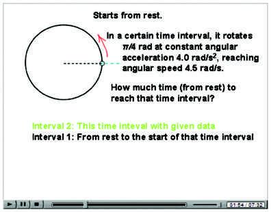
10.2 ROTATION WITH CONSTANT ANGULAR ACCELERATION 279
Rotation with Constant Angular Acceleration 279
10.3 RELATING THE LINEAR AND ANGULAR VARIABLES 281
Relating the Linear and Angular Variables 281
10.4 KINETIC ENERGY OF ROTATION 285
Kinetic Energy of Rotation 285
10.5 CALCULATING THE ROTATIONAL INERTIA 286
Calculating the Rotational Inertia 287
10.6 TORQUE 291
Torque 291
10.7 NEWTON’S SECOND LAW FOR ROTATION 292
Newton’s Second Law for Rotation 293
10.8 WORK AND ROTATIONAL KINETIC ENERGY 296
Work and Rotational Kinetic Energy 297
REVIEW & SUMMARY 299 QUESTIONS 300 PROBLEMS 301
11 Rolling, Torque, and Angular Momentum 310
11.1 ROLLING AS TRANSLATION AND ROTATION COMBINED 310
What Is Physics? 310
Rolling as Translation and Rotation Combined 310
11.2 FORCES AND KINETIC ENERGY OF ROLLING 313
The Kinetic Energy of Rolling 313
The Forces of Rolling 314
11.3 THE YO-YO 316
The Yo-Yo 317
11.4 TORQUE REVISITED 317
Torque Revisited 318
11.5 ANGULAR MOMENTUM 320
Angular Momentum 320
11.6 NEWTON’S SECOND LAW IN ANGULAR FORM 322
Newton’s Second Law in Angular Form 322
11.7 ANGULAR MOMENTUM OF A RIGID BODY 325
The Angular Momentum of a System of Particles 325
The Angular Momentum of a Rigid Body
Rotating About a Fixed Axis 326
11.8 CONSERVATION OF ANGULAR MOMENTUM 328
Conservation of Angular Momentum 328
11.9 PRECESSION OF A GYROSCOPE 333
Precession of a Gyroscope 333
REVIEW & SUMMARY 334 QUESTIONS 335 PROBLEMS 336
12 Equilibrium and Elasticity 344
12.1 EQUILIBRIUM 344
What Is Physics? 344
Equilibrium 344
The Requirements of Equilibrium 346
The Center of Gravity 347
12.2 SOME EXAMPLES OF STATIC EQUILIBRIUM 349
Some Examples of Static Equilibrium 349
12.3 ELASTICITY 355
Indeterminate Structures 355
Elasticity 356
REVIEW & SUMMARY 360 QUESTIONS 360 PROBLEMS 362
13 Gravitation 372
13.1 NEWTON’S LAW OF GRAVITATION 372
What Is Physics? 372
Newton’s Law of Gravitation 373
13.2 GRAVITATION AND THE PRINCIPLE OF SUPERPOSITION 375
Gravitation and the Principle of Superposition 375
13.3 GRAVITATION NEAR EARTH’S SURFACE 377
Gravitation Near Earth’s Surface 378
13.4 GRAVITATION INSIDE EARTH 381
Gravitation Inside Earth 381
13.5 GRAVITATIONAL POTENTIAL ENERGY 383
Gravitational Potential Energy 383
13.6 PLANETS AND SATELLITES: KEPLER’S LAWS 387
Planets and Satellites: Kepler’s Laws 388
13.7 SATELLITES: ORBITS AND ENERGY 390
Satellites: Orbits and Energy 391
13.8 EINSTEIN AND GRAVITATION 393
Einstein and Gravitation 393
REVIEW & SUMMARY 396 QUESTIONS 397 PROBLEMS 399
14 Fluids 406
14.1 FLUIDS, DENSITY, AND PRESSURE 406
What Is Physics? 406
What Is a Fluid? 406
Density and Pressure 407
14.2 FLUIDS AT REST 409
Fluids at Rest 409
14.3 MEASURING PRESSURE 412
Measuring Pressure 412
14.4 PASCAL’S PRINCIPLE 413
Pascal’s Principle 413
14.5 ARCHIMEDES’ PRINCIPLE 415
Archimedes’ Principle 415
14.6 THE EQUATION OF CONTINUITY 419
Ideal Fluids in Motion 420 The Equation of Continuity 421
14.7 BERNOULLI’S EQUATION 423 Bernoulli’s Equation 424
REVIEW & SUMMARY 426 QUESTIONS 427 PROBLEMS 428
15 Oscillations 436
15.1 SIMPLE HARMONIC MOTION 436
What Is Physics? 437
Simple Harmonic Motion 437
The Force Law for Simple Harmonic Motion 442
15.2 ENERGY IN SIMPLE HARMONIC MOTION 444
Energy in Simple Harmonic Motion 444
15.3 AN ANGULAR SIMPLE HARMONIC OSCILLATOR 446
An Angular Simple Harmonic Oscillator 446
15.4 PENDULUMS, CIRCULAR MOTION 448
Pendulums 448
Simple Harmonic Motion and Uniform Circular Motion 451
15.5 DAMPED SIMPLE HARMONIC MOTION 453
Damped Simple Harmonic Motion 453
15.6 FORCED OSCILLATIONS AND RESONANCE 456
Forced Oscillations and Resonance 456
REVIEW & SUMMARY 457 QUESTIONS 458 PROBLEMS 459
16 Waves—I 468
16.1 TRANSVERSE WAVES 468
What Is Physics? 469
Types of Waves 469
Transverse and Longitudinal Waves 469
Wavelength and Frequency 470
The Speed of a Traveling Wave 473
16.2 WAVE SPEED ON A STRETCHED STRING 476
Wave Speed on a Stretched String 476
16.3 ENERGY AND POWER OF A WAVE TRAVELING ALONG A STRING 478
Energy and Power of a Wave Traveling Along a String 478
16.4 THE WAVE EQUATION 480
The Wave Equation 480
16.5 INTERFERENCE OF WAVES 482
The Principle of Superposition for Waves 483
Interference of Waves 483
16.6 PHASORS 487
Phasors 487
16.7 STANDING WAVES AND RESONANCE 490
Standing Waves 491
Standing Waves and Resonance 493
REVIEW & SUMMARY 495 QUESTIONS 496
PROBLEMS 497
17 Waves—II 505
17.1 SPEED OF SOUND 505
What Is Physics? 505
Sound Waves 505
The Speed of Sound 506
17.2 TRAVELING SOUND WAVES 508
Traveling Sound Waves 509
17.3 INTERFERENCE 511
Interference 511
17.4 INTENSITY AND SOUND LEVEL 515
Intensity and Sound Level 515
17.5 SOURCES OF MUSICAL SOUND 518
Sources of Musical Sound 518
17.6 BEATS 522
Beats 522
17.7 THE DOPPLER EFFECT 524
The Doppler Effect 525
17.8 SUPERSONIC SPEEDS, SHOCK WAVES 529
Supersonic Speeds, Shock Waves 529
REVIEW & SUMMARY 530 QUESTIONS 531 PROBLEMS 532
18 Temperature, Heat, and the First Law
of Thermodynamics 541
18.1 TEMPERATURE 541
What Is Physics? 541
Temperature 542
The Zeroth Law of Thermodynamics 542
Measuring Temperature 543
18.2 THE CELSIUS AND FAHRENHEIT SCALES 545
The Celsius and Fahrenheit Scales 546
18.3 THERMAL EXPANSION 547
Thermal Expansion 548
18.4 ABSORPTION OF HEAT 550
Temperature and Heat 551
The Absorption of Heat by Solids and Liquids 552
18.5 THE FIRST LAW OF THERMODYNAMICS 556
A Closer Look at Heat and Work 557
The First Law of Thermodynamics 559
Some Special Cases of the First Law of Thermodynamics 560
18.6 HEAT TRANSFER MECHANISMS 562
Heat Transfer Mechanisms 563
REVIEW & SUMMARY 567 QUESTIONS 569 PROBLEMS 570
19 The Kinetic Theory of Gases
19.1 AVOGADRO’S NUMBER 578
What Is Physics? 578
Avogadro’s Number 579
19.2 IDEAL GASES 579
Ideal Gases 580
578
19.3 PRESSURE, TEMPERATURE, AND RMS SPEED 583
Pressure, Temperature, and RMS Speed 583
19.4 TRANSLATIONAL KINETIC ENERGY 586
Translational Kinetic Energy 586
19.5 MEAN FREE PATH 587
Mean Free Path 587
19.6 THE DISTRIBUTION OF MOLECULAR SPEEDS 589
The Distribution of Molecular Speeds 590
19.7 THE MOLAR SPECIFIC HEATS OF AN IDEAL GAS 593
The Molar Specific Heats of an Ideal Gas 593
19.8 DEGREES OF FREEDOM AND MOLAR SPECIFIC HEATS 597
Degrees of Freedom and Molar Specific Heats 597
A Hint of Quantum Theory 600
19.9 THE ADIABATIC EXPANSION OF AN IDEAL GAS 600
The Adiabatic Expansion of an Ideal Gas 601
REVIEW & SUMMARY 605 QUESTIONS 606 PROBLEMS 606
20 Entropy and the Second Law of Thermodynamics 613
20.1 ENTROPY 613
What Is Physics? 614
Irreversible Processes and Entropy 614
Change in Entropy 615
The Second Law of Thermodynamics 619
20.2 ENTROPY IN THE REAL WORLD: ENGINES 620
Entropy in the Real World: Engines 621
20.3 REFRIGERATORS AND REAL ENGINES 626
Entropy in the Real World: Refrigerators 627
The Efficiencies of Real Engines 628
20.4 A STATISTICAL VIEW OF ENTROPY 629
A Statistical View of Entropy 629
REVIEW & SUMMARY 633 QUESTIONS 634 PROBLEMS 635
APPENDICES
A The International System of Units (SI) A-1
B Some Fundamental Constants of Physics A-3
C Some Astronomical Data A-4
D Conversion Factors A-5
E Mathematical Formulas A-9
F Properties of the Elements A-12
G Periodic Table of the Elements A-15
ANSWERS
To Checkpoints and Odd-Numbered Questions and Problems AN-1
INDEX I-1
As requested by instructors, here is a new edition of the textbook originated by David Halliday and Robert Resnick in 1963 and that I used as a first-year student at MIT. (Gosh, time has flown by.)
Constructing this new edition allowed me to discover many delightful new examples and revisit a few favorites from my earlier eight editions. Here below are some highlights of this 12th edition.
Figure 10.39 What tension was required by the Achilles tendons in Michael Jackson in his gravitydefying 45º lean during his video Smooth Criminals?
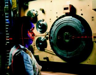
Figure 34.5.4 In functional near infrared spectroscopy (fNIRS), a person wears a close-fitting cap with LEDs emitting in the near infrared range. The light can penetrate into the outer layer of the brain and reveal when that portion is activated by a given activity, from playing baseball to flying an airplane.
10.7.2 What is the increase in the tension of the Achilles tendons when high heels are worn?
Figure 9.65 Falling is a chronic and serious condition among skateboarders, in-line skaters, elderly people, people with seizures, and many others. Often, they fall onto one outstretched hand, fracturing the wrist. What fall height can result in such fracture?
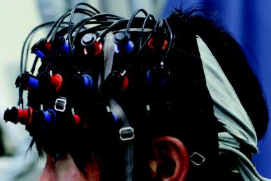
Figure 28.5.2 Fast-neutron therapy is a promising weapon against salivary gland malignancies. But how can electrically neutral particles be accelerated to high speeds?
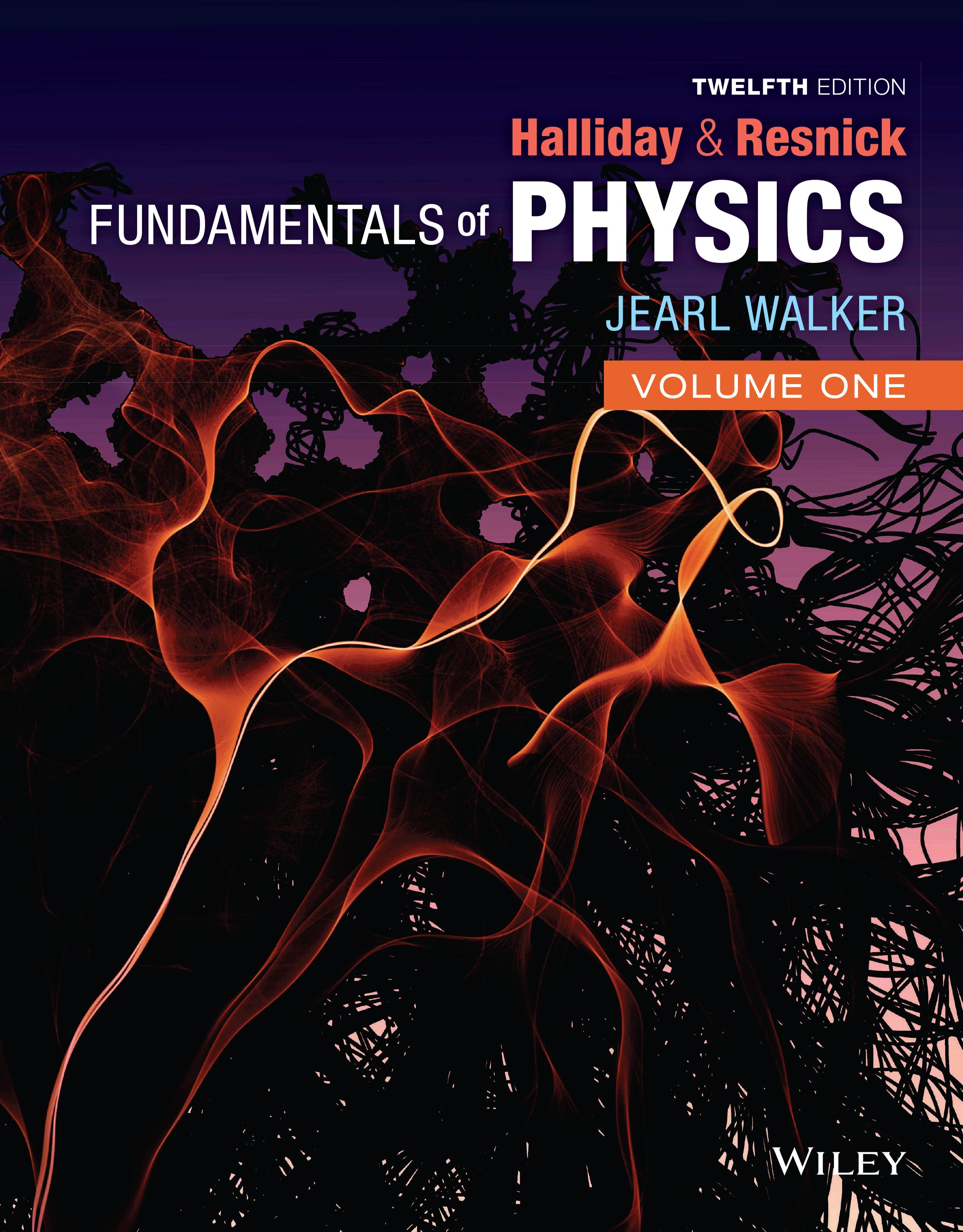
Figure 29.63 Parkinson’s disease and other brain disorders have been treated with transcranial magnetic stimulation in which pulsed magnetic fields force neurons several centimeters deep to discharge.
Figure 2.37 How should autonomous car B be programmed so that it can safely pass car A without being in danger from oncoming car C?
Figure 4.39 In a Pittsburgh left, a driver in the opposite lane anticipates the onset of the green light and rapidly pulls in front of your car during the red light. In a crash reconstruction, how soon before the green did the other driver start the turn?
Figure 9.6.4 The most dangerous car crash is a head-on crash. In a head-on crash of cars of identical mass, by how much does the probability of a fatality of a driver decrease if the driver has a passenger in the car?
Figure
Evgeniy
In addition, there are problems dealing with
• remote detection of the fall of an elderly person,
• the illusion of a rising fastball,
• hitting a fastball in spite of momentary vision loss,
• ship squat in which a ship rides lower in the water in a channel,
• the common danger of a bicyclist disappearing from view at an intersection,
• measurement of thunderstorm potentials with muons, and more.
WHAT’S IN THE BOOK
• Checkpoints, one for every module
• Sample problems
• Review and summary at the end of each chapter
• Nearly 300 new end-of-chapter problems
In constructing this new edition, I focused on several areas of research that intrigue me and wrote new text discussions and many new homework problems. Here are a few research areas:
We take a look at the first image of a black hole (for which I have waited my entire life), and then we examine gravitational waves (something I discussed with Rainer Weiss at MIT when I worked in his lab several years before he came up with the idea of using an interferometer as a wave detector).
I wrote a new sample problem and several homework problems on autonomous cars where a computer system must calculate safe driving procedures, such as passing a slow car with an oncoming car in the passing lane.
I explored cancer radiation therapy, including the use of Augur‐Meitner electrons that were first understood by Lise Meitner.
I combed through many thousands of medical, engineering, and physics research articles to find clever ways of looking inside the human body without major invasive surgery. Some are listed in the index under “medical procedures and equipment.” Here are three examples:
(1) Robotic surgery using single‐port incisions and optical fibers now allows surgeons to access internal organs, with patient recovery times of only hours instead of days or weeks as with previous surgery techniques.
(2) Transcranial magnetic stimulation is being used to treat chronic depression, Parkinson’s disease, and other brain malfunctions by applying pulsed magnetic fields from coils near the scalp to force neurons several centimeters deep to discharge.
(3) Magnetoencephalography (MEG) is being used to monitor a person’s brain as the person performs a task such as reading. The task causes weak electrical pulses to be sent along conducting paths between brain cells, and each pulse produces a weak magnetic field that is detected by extremely sensitive SQUIDs.
Physics Circus
THE WILEYPLUS ADVANTAGE
WileyPLUS is a research-based online environment for effective teaching and learning. The customization features, quality question banks, interactive eTextbook, and analytical tools allow you to quickly create a customized course that tracks student learning trends. Your students can stay engaged and on track with the use of intuitive tools like the syncing calendar and the student mobile app. Wiley is committed to providing accessible resources to instructors and students. As such, all Wiley educational products and services are born accessible, designed for users of all abilities.
Links Between Homework Problems and Learning Objectives In WileyPLUS, every question and problem at the end of the chapter is linked to a learning objective, to answer the (usually unspoken) questions, “Why am I working this problem? What am I supposed to learn from it?” By being explicit about a problem’s purpose, I believe that a student might better transfer the learning objective to other problems with a different wording but the same key idea. Such transference would help defeat the common trouble that a student learns to work a particular problem but cannot then apply its key idea to a problem in a different setting.
Animations of one of the key figures in each chapter. Here in the book, those figures are flagged with the swirling icon. In the online chapter in WileyPLUS, a mouse click begins the animation. I have chosen the figures that are rich in information so that a student can see the physics in action and played out over a minute or two instead of just being flat on a printed page. Not only does this give life to the physics, but the animation can be repeated as many times as a student wants.
Video Illustrations David Maiullo of Rutgers University has created video versions of approximately 30 of the photographs and figures from the chapters. Much of physics is the study of things that move, and video can often provide better representation than a static photo or figure.
Videos I have made well over 1500 instructional videos, with more coming. Students can watch me draw or type on the screen as they hear me talk about a solution, tutorial, sample problem, or review, very much as they would experience were they sitting next to me in my office while I worked out something on a notepad. An instructor’s lectures and tutoring will always be the most valuable learning tools, but my videos are available 24 hours a day, 7 days a week, and can be repeated indefinitely.
• Video tutorials on subjects in the chapters. I chose the subjects that challenge the students the most, the ones that my students scratch their heads about.
• Video reviews of high school math, such as basic algebraic manipulations, trig functions, and simultaneous equations.
• Video introductions to math, such as vector multiplication, that will be new to the students.
• Video presentations of sample problems. My intent is to work out the physics, starting with the key ideas instead of just grabbing a formula. However, I also want to demonstrate how to read a sample problem, that is, how to read technical material to learn problem-solving procedures that can be transferred to other types of problems.
• Video solutions to 20% of the end-of chapter problems. The availability and timing of these solutions are controlled by the instructor. For example, they might be available after a homework deadline or a quiz. Each solution is not simply a plug-and-chug recipe. Rather I build a solution from the key ideas to the first step of reasoning and to a final solution. The student learns not just how to solve a particular problem but how to tackle any problem, even those that require physics courage
• Video examples of how to read data from graphs (more than simply reading off a number with no comprehension of the physics).
• Many of the sample problems in the textbook are available online in both reading and video formats
Problem-Solving Help I have written a large number of resources for WileyPLUS designed to help build the students’ problem-solving skills.
• Hundreds of additional sample problems. These are available as stand-alone resources but (at the discretion of the instructor) they are also linked out of the homework problems. So, if a homework problem deals with, say, forces on a block on a ramp, a link to a related sample problem is provided. However, the sample problem is not just a replica of the homework problem and thus does not provide a solution that can be merely duplicated without comprehension.

• GO Tutorials for 15% of the end-of-chapter homework problems. In multiple steps, I lead a student through a homework problem, starting with the key ideas and giving hints when wrong answers are submitted. However, I purposely leave the last step (for the final answer) to the students so that they are responsible at the end. Some online tutorial systems trap a student when wrong answers are given, which can generate a lot of frustration. My GO Tutorials are not traps, because at any step along the way, a student can return to the main problem.
• Hints on every end-of-chapter homework problem are available (at the discretion of the instructor). I wrote these as true hints about the main ideas and the general procedure for a solution, not as recipes that provide an answer without any comprehension.
• Pre-lecture videos. At an instructor’s discretion, a pre-lecture video is available for every module. Also, assignable questions are available to accompany these videos. The videos were produced by Melanie Good of the University of Pittsburgh.
Evaluation Materials
• Pre-lecture reading questions are available in WileyPLUS for each chapter section. I wrote these so that they do not require analysis or any deep understanding; rather they simply test whether a student has read the section. When a student opens up a section, a randomly chosen reading question (from a bank of questions) appears at the end. The instructor can decide whether the question is part of the grading for that section or whether it is just for the benefit of the student.
• Checkpoints are available within each chapter module. I wrote these so that they require analysis and decisions about the physics in the section. Answers are provided in the back of the book.
• All end-of-chapter homework problems (and many more problems) are available in WileyPLUS. The instructor can construct a homework assignment and control how it is graded when the answers are submitted online. For example, the instructor controls the deadline for submission and how many attempts a student is allowed on an answer. The instructor also controls which, if any, learning aids are available with each homework problem. Such links can include hints, sample problems, in-chapter reading materials, video tutorials, video math reviews, and even video solutions (which can be made available to the students after, say, a homework deadline).
• Symbolic notation problems that require algebraic answers are available in every chapter.
• All end-of-chapter homework questions are available for assignment in WileyPLUS. These questions (in a multiple-choice format) are designed to evaluate the students’ conceptual understanding.
• Interactive Exercises and Simulations by Brad Trees of Ohio Wesleyan University. How do we help students understand challenging concepts in physics? How do we motivate students to engage with core content in a meaningful way? The simulations are intended to address these key questions. Each module in the Etext is linked to one or more simulations that convey concepts visually. A simulation depicts a physical situation in which time dependent phenomena are animated and information is presented in multiple representations including a visual representation of the physical system as well as a plot of related variables. Often, adjustable parameters allow the user to change a property of the system and to see the effects of that change on the subsequent behavior. For visual learners, the simulations provide an opportunity to “see” the physics in action. Each simulation is also linked to a set of interactive exercises, which guide the student through a deeper interaction with the physics underlying the simulation. The exercises consist of a series of practice questions with feedback and detailed solutions. Instructors may choose to assign the exercises for practice, to recommend the exercises to students as additional practice, and to show individual simulations during class time to demonstrate a concept and to motivate class discussion.
Icons for Additional Help When worked-out solutions are provided either in print or electronically for certain of the odd-numbered problems, the statements for those problems include an icon to alert both student and instructor. There are also icons indicating which problems have a GO Tutorial or a link to the The Flying Circus of Physics, which require calculus, and which involve a biomedical application. An icon guide is provided here and at the beginning of each set of problems.
Tutoring problem available (at instructor’s discretion) in WileyPLUS
Worked-out solution available in Student Solutions Manual
M Medium H
Additional information available in The Flying Circus of Physics and at flyingcircusofphysics.com
FUNDAMENTALS OF PHYSICS—FORMAT OPTIONS
Fundamentals of Physics was designed to optimize students’ online learning experience. We highly recommend that students use the digital course within WileyPLUS as their primary course material. Here are students’ purchase options:
• 12th Edition WileyPLUS course
• Fundamentals of Physics Looseleaf Print Companion bundled with WileyPLUS
• Fundamentals of Physics volume 1 bundled with WileyPLUS
• Fundamentals of Physics volume 2 bundled with WileyPLUS
• Fundamentals of Physics Vitalsource Etext
SUPPLEMENTARY MATERIALS AND ADDITIONAL RESOURCES
Supplements for the instructor can be obtained online through WileyPLUS or by contacting your Wiley representative. The following supplementary materials are available for this edition:
Instructor’s Solutions Manual by Sen-Ben Liao, Lawrence Livermore National Laboratory. This manual provides worked-out solutions for all problems found at the end of each chapter. It is available in both MSWord and PDF.
• Instructor’s Manual This resource contains lecture notes outlining the most important topics of each chapter; demonstration experiments; laboratory and computer projects; film and video sources; answers to all questions, exercises, problems, and checkpoints; and a correlation guide to the questions, exercises, and problems in the previous edition. It also contains a complete list of all problems for which solutions are available to students.
• Classroom Response Systems (“Clicker”) Questions by David Marx, Illinois State University. There are two sets of questions available: Reading Quiz questions and Interactive Lecture questions.The Reading Quiz questions are intended to be relatively straightforward for any student who reads the assigned material. The Interactive Lecture questions are intended for use in an interactive lecture setting.
• Wiley Physics Simulations by Andrew Duffy, Boston University and John Gastineau, Vernier Software. This is a collection of 50 interactive simulations (Java applets) that can be used for classroom demonstrations.
• Wiley Physics Demonstrations by David Maiullo, Rutgers University. This is a collection of digital videos of 80 standard physics demonstrations. They can be shown in class or accessed from WileyPLUS. There is an accompanying Instructor’s Guide that includes “clicker” questions.
• Test Bank by Suzanne Willis, Northern Illinois University. The Test Bank includes nearly 3,000 multiple-choice questions. These items are also available in the Computerized Test Bank, which provides full editing features to help you customize tests (available in both IBM and Macintosh versions).
• All text illustrations suitable for both classroom projection and printing.
• Lecture PowerPoint Slides These PowerPoint slides serve as a helpful starter pack for instructors, outlining key concepts and incorporating figures and equations from the text.
STUDENT SUPPLEMENTS
Student Solutions Manual (ISBN 9781119455127) by Sen-Ben Liao, Lawrence Livermore National Laboratory. This manual provides students with complete worked-out solutions to 15 percent of the problems found at the end of each chapter within the text. The Student Solutions Manual for the 12th edition is written using an innovative approach called TEAL, which stands for Think, Express, Analyze, and Learn. This learning strategy was originally developed at the Massachusetts Institute of Technology and has proven to be an effective learning tool for students. These problems with TEAL solutions are indicated with an SSM icon in the text.
Introductory Physics with Calculus as a Second Language (ISBN 9780471739104) Mastering Problem Solving by Thomas Barrett of Ohio State University. This brief paperback teaches the student how to approach problems more efficiently and effectively. The student will learn how to recognize common patterns in physics problems, break problems down into manageable steps, and apply appropriate techniques. The book takes the student step by step through the solutions to numerous examples.
A great many people have contributed to this book. Sen-Ben Liao of Lawrence Livermore National Laboratory, James Whitenton of Southern Polytechnic State University, and Jerry Shi of Pasadena City College performed the Herculean task of working out solutions for every one of the homework problems in the book. At John Wiley publishers, the book received support from John LaVacca and Jennifer Yee, the editors who oversaw the entire project from start to finish, as well as Senior Managing Editor Mary Donovan and Editorial Assistant Samantha Hart. We thank Patricia Gutierrez and the Lumina team, for pulling all the pieces together during the complex production process, and Course Developers Corrina Santos and Kimberly Eskin, for masterfully developing the WileyPLUS course and online resources, We also thank Jon Boylan for the art and cover design; Helen Walden for her copyediting; and Donna Mulder for her proofreading.
Finally, our external reviewers have been outstanding and we acknowledge here our debt to each member of that team.
Maris A. Abolins, Michigan State University
Jonathan Abramson, Portland State University
Omar Adawi, Parkland College
Edward Adelson, Ohio State University
Nural Akchurin, Texas Tech
Yildirim Aktas, University of North Carolina-Charlotte
Barbara Andereck, Ohio Wesleyan University
Tetyana Antimirova, Ryerson University
Mark Arnett, Kirkwood Community College
Stephen R. Baker, Naval Postgraduate School
Arun Bansil, Northeastern University
Richard Barber, Santa Clara University
Neil Basecu, Westchester Community College
Anand Batra, Howard University
Sidi Benzahra, California State Polytechnic University, Pomona
Kenneth Bolland, The Ohio State University
Richard Bone, Florida International University
Michael E. Browne, University of Idaho
Timothy J. Burns, Leeward Community College
Joseph Buschi, Manhattan College
George Caplan, Wellesley College
Philip A. Casabella, Rensselaer Polytechnic Institute
Randall Caton, Christopher Newport College
John Cerne, University at Buffalo, SUNY
Roger Clapp, University of South Florida
W. R. Conkie, Queen’s University
Renate Crawford, University of Massachusetts-Dartmouth
Mike Crivello, San Diego State University
Robert N. Davie, Jr., St. Petersburg Junior College
Cheryl K. Dellai, Glendale Community College
Eric R. Dietz, California State University at Chico
N. John DiNardo, Drexel University
Eugene Dunnam, University of Florida
Robert Endorf, University of Cincinnati
F. Paul Esposito, University of Cincinnati
Jerry Finkelstein, San Jose State University
Lev Gasparov, University of North Florida
Brian Geislinger, Gadsden State Community College
Corey Gerving, United States Military Academy
Robert H. Good, California State University-Hayward
Michael Gorman, University of Houston
Benjamin Grinstein, University of California, San Diego
John B. Gruber, San Jose State University
Ann Hanks, American River College
Randy Harris, University of California-Davis
Samuel Harris, Purdue University
Harold B. Hart, Western Illinois University
Rebecca Hartzler, Seattle Central Community College
Kevin Hope, University of Montevallo
John Hubisz, North Carolina State University
Joey Huston, Michigan State University
David Ingram, Ohio University
Shawn Jackson, University of Tulsa
Hector Jimenez, University of Puerto Rico
Sudhakar B. Joshi, York University
Leonard M. Kahn, University of Rhode Island
Rex Joyner, Indiana Institute of Technology
Michael Kalb, The College of New Jersey
Richard Kass, The Ohio State University
M.R. Khoshbin-e-Khoshnazar, Research Institution for Curriculum Development and Educational Innovations (Tehran)
Sudipa Kirtley, Rose-Hulman Institute
Leonard Kleinman, University of Texas at Austin
Craig Kletzing, University of Iowa
Peter F. Koehler, University of Pittsburgh
Arthur Z. Kovacs, Rochester Institute of Technology
Kenneth Krane, Oregon State University
Hadley Lawler, Vanderbilt University
Priscilla Laws, Dickinson College
Edbertho Leal, Polytechnic University of Puerto Rico
Vern Lindberg, Rochester Institute of Technology
Peter Loly, University of Manitoba
Stuart Loucks, American River College
Laurence Lurio, Northern Illinois University
James MacLaren, Tulane University
Ponn Maheswaranathan, Winthrop University
Andreas Mandelis, University of Toronto
Robert R. Marchini, Memphis State University
Andrea Markelz, University at Buffalo, SUNY
Paul Marquard, Caspar College
David Marx, Illinois State University
Dan Mazilu, Washington and Lee University
Jeffrey Colin McCallum, The University of Melbourne
Joe McCullough, Cabrillo College
James H. McGuire, Tulane University
David M. McKinstry, Eastern Washington University
Jordon Morelli, Queen’s University
Eugene Mosca, United States Naval Academy
Carl E. Mungan, United States Naval Academy
Eric R. Murray, Georgia Institute of Technology, School of Physics
James Napolitano, Rensselaer Polytechnic Institute
Amjad Nazzal, Wilkes University
Allen Nock, Northeast Mississippi Community College
Blaine Norum, University of Virginia
Michael O’Shea, Kansas State University
Don N. Page, University of Alberta
Patrick Papin, San Diego State University
Kiumars Parvin, San Jose State University
Robert Pelcovits, Brown University
Oren P. Quist, South Dakota State University
Elie Riachi, Fort Scott Community College
Joe Redish, University of Maryland
Andrew Resnick, Cleveland State University
Andrew G. Rinzler, University of Florida
Timothy M. Ritter, University of North Carolina at Pembroke
Dubravka Rupnik, Louisiana State University
Robert Schabinger, Rutgers University
Ruth Schwartz, Milwaukee School of Engineering
Thomas M. Snyder, Lincoln Land Community College
Carol Strong, University of Alabama at Huntsville
Anderson Sunda-Meya, Xavier University of Louisiana
Dan Styer, Oberlin College
Nora Thornber, Raritan Valley Community College
Frank Wang, LaGuardia Community College
Keith Wanser, California State University Fullerton
Robert Webb, Texas A&M University
David Westmark, University of South Alabama
Edward Whittaker, Stevens Institute of Technology
Suzanne Willis, Northern Illinois University
Shannon Willoughby, Montana State University
Graham W. Wilson, University of Kansas
Roland Winkler, Northern Illinois University
William Zacharias, Cleveland State University
Ulrich Zurcher, Cleveland State University
Measurement
1.1 MEASURING THINGS, INCLUDING LENGTHS
Learning Objectives
After reading this module, you should be able to . . .
1.1.1 Identify the base quantities in the SI system.
1.1.2 Name the most frequently used prefixes for SI units.
Key Ideas
● Physics is based on measurement of physical quantities. Certain physical quantities have been chosen as base quantities (such as length, time, and mass); each has been defined in terms of a standard and given a unit of measure (such as meter, second, and kilogram). Other physical quantities are defined in terms of the base quantities and their standards and units.
● The unit system emphasized in this book is the International System of Units (SI). The three physical quantities displayed in Table 1.1.1 are used in the early chapters. Standards, which must be both accessible and invariable, have been established for these base
What Is Physics?
1.1.3 Change units (here for length, area, and volume) by using chain-link conversions.
1.1.4 Explain that the meter is defined in terms of the speed of light in a vacuum.
quantities by international agreement. These standards are used in all physical measurement, for both the base quantities and the quantities derived from them. Scientific notation and the prefixes of Table 1.1.2 are used to simplify measurement notation.
● Conversion of units may be performed by using chain-link conversions in which the original data are multiplied successively by conversion factors written as unity and the units are manipulated like algebraic quantities until only the desired units remain.
● The meter is defined as the distance traveled by light during a precisely specified time interval.
Science and engineering are based on measurements and comparisons. Thus, we need rules about how things are measured and compared, and we need experiments to establish the units for those measurements and comparisons. One purpose of physics (and engineering) is to design and conduct those experiments. For example, physicists strive to develop clocks of extreme accuracy so that any time or time interval can be precisely determined and compared. You may wonder whether such accuracy is actually needed or worth the effort. Here is one example of the worth: Without clocks of extreme accuracy, the Global Positioning System (GPS) that is now vital to worldwide navigation would be useless.
Measuring Things
We discover physics by learning how to measure the quantities involved in physics. Among these quantities are length, time, mass, temperature, pressure, and electric current.
Quantity Unit Name Unit Symbol
Length meter m
Time second s
Mass kilogram kg
We measure each physical quantity in its own units, by comparison with a standard. The unit is a unique name we assign to measures of that quantity— for example, meter (m) for the quantity length. The standard corresponds to exactly 1.0 unit of the quantity. As you will see, the standard for length, which corresponds to exactly 1.0 m, is the distance traveled by light in a vacuum during a certain fraction of a second. We can define a unit and its standard in any way we care to. However, the important thing is to do so in such a way that scientists around the world will agree that our definitions are both sensible and practical.
Once we have set up a standard—say, for length—we must work out procedures by which any length whatever, be it the radius of a hydrogen atom, the wheelbase of a skateboard, or the distance to a star, can be expressed in terms of the standard. Rulers, which approximate our length standard, give us one such procedure for measuring length. However, many of our comparisons must be indirect. You cannot use a ruler, for example, to measure the radius of an atom or the distance to a star.
Base Quantities. There are so many physical quantities that it is a problem to organize them. Fortunately, they are not all independent; for example, speed is the ratio of a length to a time. Thus, what we do is pick out—by international agreement—a small number of physical quantities, such as length and time, and assign standards to them alone. We then define all other physical quantities in terms of these base quantities and their standards (called base standards). Speed, for example, is defined in terms of the base quantities length and time and their base standards.
Base standards must be both accessible and invariable. If we define the length standard as the distance between one’s nose and the index finger on an outstretched arm, we certainly have an accessible standard—but it will, of course, vary from person to person. The demand for precision in science and engineering pushes us to aim first for invariability. We then exert great effort to make duplicates of the base standards that are accessible to those who need them.
The International System of Units
In 1971, the 14th General Conference on Weights and Measures picked seven quantities as base quantities, thereby forming the basis of the International System of Units, abbreviated SI from its French name and popularly known as the metric system. Table 1.1.1 shows the units for the three base quantities— length, mass, and time—that we use in the early chapters of this book. These units were defined to be on a “human scale.”
Many SI derived units are defined in terms of these base units. For example, the SI unit for power, called the watt (W), is defined in terms of the base units for mass, length, and time. Thus, as you will see in Chapter 7,
where the last collection of unit symbols is read as kilogram-meter squared per second cubed.
To express the very large and very small quantities we often run into in physics, we use scientific notation, which employs powers of 10. In this notation,
Scientific notation on computers sometimes takes on an even briefer look, as in 3.56 E9 and 4.92 E–7, where E stands for “exponent of ten.” It is briefer still on some calculators, where E is replaced with an empty space.
Table 1.1.1 Units for Three SI Base Quantities
As a further convenience when dealing with very large or very small measurements, we use the prefixes listed in Table 1.1.2. As you can see, each prefix represents a certain power of 10, to be used as a multiplication factor. Attaching a prefix to an SI unit has the effect of multiplying by the associated factor. Thus, we can express a particular electric power as
1.27 × 10⁹ watts = 1.27 gigawatts = 1.27 GW (1.1.4)
or a particular time interval as
2.35 × 10 9 s = 2.35 nanoseconds = 2.35 ns. (1.1.5)
Some prefixes, as used in milliliter, centimeter, kilogram, and megabyte, are probably familiar to you.
Changing Units
We often need to change the units in which a physical quantity is expressed. We do so by a method called chain-link conversion. In this method, we multiply the original measurement by a conversion factor (a ratio of units that is equal to unity). For example, because 1 min and 60 s are identical time intervals, we have 1 min 60 s = 1 and 60 s 1 min = 1.
Thus, the ratios (1 min)/(60 s) and (60 s)/(1 min) can be used as conversion factors. This is not the same as writing 1 60 = 1 or 60 = 1; each number and its unit must be treated together.
Because multiplying any quantity by unity leaves the quantity unchanged, we can introduce conversion factors wherever we find them useful. In chain-link conversion, we use the factors to cancel unwanted units. For example, to convert 2 min to seconds, we have
2 min = (2 min)(1) = (2 min)( 60 s 1 min ) = 120 s.
(1.1.6)
If you introduce a conversion factor in such a way that unwanted units do not cancel, invert the factor and try again. In conversions, the units obey the same algebraic rules as variables and numbers.
Appendix D gives conversion factors between SI and other systems of units, including non-SI units still used in the United States. However, the conversion factors are written in the style of “1 min = 60 s” rather than as a ratio. So, you need to decide on the numerator and denominator in any needed ratio.
Length
In 1792, the newborn Republic of France established a new system of weights and measures. Its cornerstone was the meter, defined to be one ten-millionth of the distance from the north pole to the equator. Later, for practical reasons, this Earth standard was abandoned and the meter came to be defined as the distance between two fine lines engraved near the ends of a platinum–iridium bar, the standard meter bar, which was kept at the International Bureau of Weights and Measures near Paris. Accurate copies of the bar were sent to standardizing laboratories throughout the world. These secondary standards were used to produce other, still more accessible standards, so that ultimately every
Table 1.1.2 Prefixes for SI Units Factor
yotta-
zetta-
exa-
peta-
tera-
giga-
mega-
kilo-
hecto-
deka-
1 deci-
2 centi-
10 3 milli-
10 6 micro-
10 9 nano- n 10 12 pico- p 10 15 femto- f
10 18 atto- a 10 21 zepto- z 10 24 yocto- y
aThe most frequently used prefixes are shown in bold type.
Table 1.1.3 Some Approximate Lengths
Measurement
Length in Meters
Distance to the first galaxies formed 2 × 1026
Distance to the Andromeda galaxy 2 × 10²²
Distance to the nearby star Proxima Centauri 4 × 10¹⁶
Distance to Pluto 6 × 10¹²
Radius of Earth 6 × 10⁶
Height of Mt. Everest 9 × 10³
Thickness of this page 1 × 10 4
Length of a typical virus 1 × 10 8
Radius of a hydrogen atom
5 × 10 11
Radius of a proton 1 × 10 15
measuring device derived its authority from the standard meter bar through a complicated chain of comparisons.
Eventually, a standard more precise than the distance between two fine scratches on a metal bar was required. In 1960, a new standard for the meter, based on the wavelength of light, was adopted. Specifically, the standard for the meter was redefined to be 1 650 763.73 wavelengths of a particular orange-red light emitted by atoms of krypton-86 (a particular isotope, or type, of krypton) in a gas discharge tube that can be set up anywhere in the world. This awkward number of wavelengths was chosen so that the new standard would be close to the old meter-bar standard.
By 1983, however, the demand for higher precision had reached such a point that even the krypton-86 standard could not meet it, and in that year a bold step was taken. The meter was redefined as the distance traveled by light in a specified time interval. In the words of the 17th General Conference on Weights and Measures:
The meter is the length of the path traveled by light in a vacuum during a time interval of 1/299 792 458 of a second.
This time interval was chosen so that the speed of light c is exactly c = 299 792 458 m/s.
Measurements of the speed of light had become extremely precise, so it made sense to adopt the speed of light as a defined quantity and to use it to redefine the meter.
Table 1.1.3 shows a wide range of lengths, from that of the universe (top line) to those of some very small objects.
Significant Figures and Decimal Places
Suppose that you work out a problem in which each value consists of two digits. Those digits are called significant figures and they set the number of digits that you can use in reporting your final answer. With data given in two significant figures, your final answer should have only two significant figures. However, depending on the mode setting of your calculator, many more digits might be displayed. Those extra digits are meaningless.
In this book, final results of calculations are often rounded to match the least number of significant figures in the given data. (However, sometimes an extra significant figure is kept.) When the leftmost of the digits to be discarded is 5 or more, the last remaining digit is rounded up; otherwise it is retained as is. For example, 11.3516 is rounded to three significant figures as 11.4 and 11.3279 is rounded to three significant figures as 11.3. (The answers to sample problems in this book are usually presented with the symbol = instead of ≈ even if rounding is involved.)
When a number such as 3.15 or 3.15 × 10³ is provided in a problem, the number of significant figures is apparent, but how about the number 3000? Is it known to only one significant figure (3 × 10³)? Or is it known to as many as four significant figures (3.000 × 10³)? In this book, we assume that all the zeros in such given numbers as 3000 are significant, but you had better not make that assumption elsewhere.
Don’t confuse significant figures with decimal places. Consider the lengths 35.6 mm, 3.56 m, and 0.00356 m. They all have three significant figures but they have one, two, and five decimal places, respectively.
Sample Problem 1.1.1 Estimating order of magnitude, ball of string
The world’s largest ball of string is about 2 m in radius. To the nearest order of magnitude, what is the total length L of the string in the ball?
KEY IDEA
We could, of course, take the ball apart and measure the total length L, but that would take great effort and make the ball’s builder most unhappy. Instead, because we want only the nearest order of magnitude, we can estimate any quantities required in the calculation.
Calculations: Let us assume the ball is spherical with radius R = 2 m. The string in the ball is not closely packed (there are uncountable gaps between adjacent sections of string). To allow for these gaps, let us somewhat overestimate the cross-sectional area of the string by assuming the cross section is square, with an edge length d = 4 mm.
Then, with a cross-sectional area of d2 and a length L, the string occupies a total volume of
V = (cross-sectional area)(length) = d2L.
This is approximately equal to the volume of the ball, given by 4 3 πR 3, which is about 4R3 because π is about 3. Thus, we have the following
d2L = 4R3 , or L = 4R 3 d 2 = 4(2 m)3 (4 × 10 3 m)2 = 2 × 10⁶ m ≈ 106 m = 103 km.
(Answer)
(Note that you do not need a calculator for such a simplified calculation.) To the nearest order of magnitude, the ball contains about 1000 km of string!
Additional examples, video, and practice available at WileyPLUS
1.2 TIME
Learning Objectives
After reading this module, you should be able to . . .
1.2.1 Change units for time by using chain-link conversions.
Key Idea
● The second is defined in terms of the oscillations of light emitted by an atomic (cesium-133) source. Accurate
Time
1.2.2 Use various measures of time, such as for motion or as determined on different clocks.
time signals are sent worldwide by radio signals keyed to atomic clocks in standardizing laboratories.
Time has two aspects. For civil and some scientific purposes, we want to know the time of day so that we can order events in sequence. In much scientific work, we want to know how long an event lasts. Thus, any time standard must be able to answer two questions: “When did it happen?” and “What is its duration?”
Table 1.2.1 shows some time intervals.
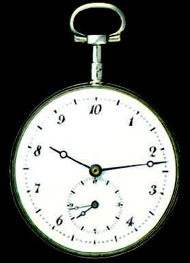
Any phenomenon that repeats itself is a possible time standard. Earth’s rotation, which determines the length of the day, has been used in this way for centuries; Fig. 1.2.1 shows one novel example of a watch based on that rotation. A quartz clock, in which a quartz ring is made to vibrate continuously, can be calibrated against Earth’s rotation via astronomical observations and used to measure time intervals in the laboratory. However, the calibration cannot be carried out with the accuracy called for by modern scientific and engineering technology.
Figure 1.2.1 When the metric system was proposed in 1792, the hour was redefined to provide a 10-hour day. The idea did not catch on. The maker of this 10-hour watch wisely provided a small dial that kept conventional 12-hour time. Do the two dials indicate the same time?
Table 1.2.1 Some Approximate Time Intervals
Measurement
Lifetime of the proton (predicted) 3 × 1040
between human heartbeats
Age of the universe 5 × 10¹⁷ Lifetime of
Figure 1.2.2 Variations in the length of the day over a 4-year period. Note that the entire vertical scale amounts to only 3 ms (= 0.003 s).
aThis is the earliest time after the big bang at which the laws of physics as we know them can be applied.
To meet the need for a better time standard, atomic clocks have been developed. An atomic clock at the National Institute of Standards and Technology (NIST) in Boulder, Colorado, is the standard for Coordinated Universal Time (UTC) in the United States. Its time signals are available by shortwave radio (stations WWV and WWVH) and by telephone (303-499-7111). Time signals (and related information) are also available from the United States Naval Observatory at website https:// www.usno.navy.mil/USNO/time. (To set a clock extremely accurately at your particular location, you would have to account for the travel time required for these signals to reach you.)
Figure 1.2.2 shows variations in the length of one day on Earth over a 4-year period, as determined by comparison with a cesium (atomic) clock. Because the variation displayed by Fig. 1.2.2 is seasonal and repetitious, we suspect the rotating Earth when there is a difference between Earth and atom as timekeepers. The variation is due to tidal effects caused by the Moon and to large-scale winds.
The 13th General Conference on Weights and Measures in 1967 adopted a standard second based on the cesium c lock:
One second is the time taken by 9 192 631 770 oscillations of the light (of a specified wavelength) emitted by a cesium-133 atom.
Atomic clocks are so consistent that, in principle, two cesium clocks would have to run for 6000 years before their readings would differ by more than 1 s. Even such accuracy pales in comparison with that of clocks currently being developed; their precision may be 1 part in 1018—that is, 1 s in 1 × 10¹⁸ s (which is about 3 × 10¹⁰ y).
1.3 MASS
Learning Objectives
After reading this module, you should be able to . . .
1.3.1 Change units for mass by using chain-link conversions. 1.3.2 Relate density to mass and volume when the mass is uniformly distributed.
Steven Pitkin
Steven Pitkin
Key Ideas
● The kilogram is defined in terms of a platinum–iridium standard mass kept near Paris. For measurements on an atomic scale, the atomic mass unit, defined in terms of the atom carbon-12, is usually used.
Mass
The Standard Kilogram
● The density ρ of a material is the mass per unit volume:
= m V
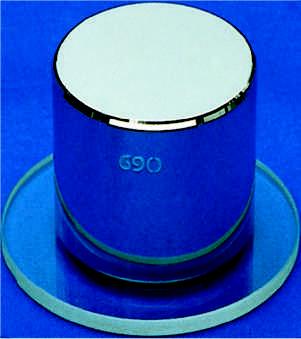
The SI standard of mass is a cylinder of platinum and iridium (Fig. 1.3.1) that is kept at the International Bureau of Weights and Measures near Paris and assigned, by international agreement, a mass of 1 kilogram. Accurate copies have been sent to standardizing laboratories in other countries, and the masses of other bodies can be determined by balancing them against a copy. Table 1.3.1 shows some masses expressed in kilograms, ranging over about 83 orders of magnitude.
The U.S. copy of the standard kilogram is housed in a vault at NIST. It is removed, no more than once a year, for the purpose of checking duplicate copies that are used elsewhere. Since 1889, it has been taken to France twice for recomparison with the primary standard.
Kibble Balance
A far more accurate way of measuring mass is now being adopted. In a Kibble balance (named after its inventor Brian Kibble), a standard mass can be measured when the downward pull on it by gravity is balanced by an upward force from a magnetic field due to an electrical current. The precision of this technique comes from the fact that the electric and magnetic properties can be determined in terms of quantum mechanical quantities that have been precisely defined or measured. Once a standard mass is measured, it can be sent to other labs where the masses of other bodies can be determined from it.
A Second Mass Standard
The masses of atoms can be compared with one another more precisely than they can be compared with the standard kilogram. For this reason, we have a second mass standard. It is the carbon-12 atom, which, by international agreement, has been assigned a mass of 12 atomic mass units (u). The relation between the two units is
1 u = 1.660 538 86 × 10 27 kg,
Figure 1.3.1 The international 1 kg standard of mass, a platinum–iridium cylinder 3.9 cm in height and in diameter.
Table 1.3.1 Some Approximate Masses
Object
(1.3.1)
with an uncertainty of ±10 in the last two decimal places. Scientists can, with reasonable precision, experimentally determine the masses of other atoms relative to the mass of carbon-12. What we presently lack is a reliable means of extending that precision to more common units of mass, such as a kilogram.
Density
As we shall discuss further in Chapter 14, density ρ (lowercase Greek letter rho) is the mass per unit volume:
Densities are typically listed in kilograms per cubic meter or grams per cubic centimeter. The density of water (1.00 gram per cubic centimeter) is often used as a comparison. Fresh snow has about 10% of that density; platinum has a density that is about 21 times that of water.
Courtesy Bureau International des Poids et Mesures. Reproduced with permission of the BIPM.
Courtesy of Bureau International des Poids et Mesures. Reproduced with permission of the BIPM.
Review & Summary
Measurement in Physics Physics is based on measurement of physical quantities. Certain physical quantities have been chosen as base quantities (such as length, time, and mass); each has been defined in terms of a standard and given a unit of measure (such as meter, second, and kilogram). Other physical quantities are defined in terms of the base quantities and their standards and units.
SI Units The unit system emphasized in this book is the International System of Units (SI). The three physical quantities displayed in Table 1.1.1 are used in the early chapters. Standards, which must be both accessible and invariable, have been established for these base quantities by international agreement. These standards are used in all physical measurement, for both the base quantities and the quantities derived from them. Scientific notation and the prefixes of Table 1.1.2 are used to simplify measurement notation.
Changing Units Conversion of units may be performed by using chain-link conversions in which the original data are
Problems
Tutoring problem available (at instructor’s discretion) in WileyPLUS
Worked-out solution available in Student Solutions Manual
E Easy M Medium H Hard
multiplied successively by conversion factors written as unity and the units are manipulated like algebraic quantities until only the desired units remain.
Length The meter is defined as the distance traveled by light during a precisely specified time interval.
Time The second is defined in terms of the oscillations of light emitted by an atomic (cesium-133) source. Accurate time signals are sent worldwide by radio signals keyed to atomic clocks in standardizing laboratories.
Mass The kilogram is defined in terms of a platinum–iridium standard mass kept near Paris. For measurements on an atomic scale, the atomic mass unit, defined in terms of the atom carbon-12, is usually used.
Density The density ρ of a material is the mass per unit volume:
Additional information available in The Flying Circus of Physics and at flyingcircusofphysics.com
Module 1.1
Measuring Things, Including Lengths
1 E SSM Earth is approximately a sphere of radius 6.37 × 10⁶ m. What are (a) its circumference in kilometers, (b) its surface area in square kilometers, and (c) its volume in cubic kilometers?
2 E A gry is an old English measure for length, defined as 1/10 of a line, where line is another old English measure for length, defined as 1/12 inch. A common measure for length in the publishing business is a point, defined as 1/72 inch. What is an area of 0.50 gry2 in points squared (points2)?
3 E The micrometer (1 μm) is often called the micron. (a) How many microns make up 1.0 km? (b) What fraction of a centimeter equals 1.0 μm? (c) How many microns are in 1.0 yd?
4 E Spacing in this book was generally done in units of points and picas: 12 points = 1 pica, and 6 picas = 1 inch. If a figure was misplaced in the page proofs by 0.80 cm, what was the misplacement in (a) picas and (b) points?
5 E SSM Horses are to race over a certain English meadow for a distance of 4.0 furlongs. What is the race distance in (a) rods and (b) chains? (1 furlong = 201.168 m, 1 rod = 5.0292 m, and 1 chain = 20.117 m.)
6 M You can easily convert common units and measures electronically, but you still should be able to use a conversion table, such as those in Appendix D. Table 1.1 is part of a conversion table for a system of volume measures once common in Spain; a volume of 1 fanega is equivalent to 55.501 dm3 (cubic decimeters). To complete the table, what numbers (to three significant
Requires calculus BIO Biomedical application
figures) should be entered in (a) the cahiz column, (b) the fanega column, (c) the cuartilla column, and (d) the almude column, starting with the top blank? Express 7.00 almudes in (e) medios, (f) cahizes, and (g) cubic centimeters (cm3).
7 M Hydraulic engineers in the United States often use, as a unit of volume of water, the acre-foot, defined as the volume of water that will cover 1 acre of land to a depth of 1 ft. A severe thunderstorm dumped 2.0 in. of rain in 30 min on a town of area 26 km2. What volume of water, in acre-feet, fell on the town?
8 M GO Harvard Bridge, which connects MIT with its fraternities across the Charles River, has a length of 364.4 Smoots plus one ear. The unit of one Smoot is based on the length of Oliver Reed Smoot, Jr., class of 1962, who was carried or dragged length by length across the bridge so that other pledge members of the Lambda Chi Alpha fraternity could mark off (with paint) 1-Smoot lengths along the bridge. The marks have
Table 1.1 Problem 6