All rights reserved. No part of this publication may be reproduced, stored in a retrieval system, or transmitted, in any form or by any means, electronic, mechanical, photocopying, recording or otherwise, except as permitted by law. Advice on how to obtain permission to reuse material from this title is available at http://www.wiley.com/go/permissions.
The right of Dan Binkley to be identified as the author of this work has been asserted in accordance with law.
Registered Offices
John Wiley & Sons, Inc., 111 River Street, Hoboken, NJ 07030, USA
John Wiley & Sons Ltd, The Atrium, Southern Gate, Chichester, West Sussex, PO19 8SQ, UK
Editorial Office
9600 Garsington Road, Oxford, OX4 2DQ, UK
For details of our global editorial offices, customer services, and more information about Wiley products visit us at www.wiley.com. Wiley also publishes its books in a variety of electronic formats and by print-on-demand. Some content that appears in standard print versions of this book may not be available in other formats.
Limit of Liability/Disclaimer of Warranty
The contents of this work are intended to further general scientific research, understanding, and discussion only and are not intended and should not be relied upon as recommending or promoting scientific method, diagnosis, or treatment by physicians for any particular patient. In view of ongoing research, equipment modifications, changes in governmental regulations, and the constant flow of information relating to the use of medicines, equipment, and devices, the reader is urged to review and evaluate the information provided in the package insert or instructions for each medicine, equipment, or device for, among other things, any changes in the instructions or indication of usage and for added warnings and precautions. While the publisher and authors have used their best efforts in preparing this work, they make no representations or warranties with respect to the accuracy or completeness of the contents of this work and specifically disclaim all warranties, including without limitation any implied warranties of merchantability or fitness for a particular purpose. No warranty may be created or extended by sales representatives, written sales materials or promotional statements for this work. The fact that an organization, website, or product is referred to in this work as a citation and/or potential source of further information does not mean that the publisher and authors endorse the information or services the organization, website, or product may provide or recommendations it may make. This work is sold with the understanding that the publisher is not engaged in rendering professional services. The advice and strategies contained herein may not be suitable for your situation. You should consult with a specialist where appropriate. Further, readers should be aware that websites listed in this work may have changed or disappeared between when this work was written and when it is read. Neither the publisher nor authors shall be liable for any loss of profit or any other commercial damages, including but not limited to special, incidental, consequential, or other damages.
Library of Congress Cataloging-in-Publication Data
Names: Binkley, Dan, author. | John Wiley & Sons, publisher.
Title: Forest ecology : an evidence-based approach / Dan Binkley, School of Forestry, Northern Arizona University.
Description: First edition. | Hoboken, NJ : Wiley-Blackwell, 2021. | Includes index.
Identifiers: LCCN 2021001373 (print) | LCCN 2021001374 (ebook) | ISBN 9781119703204 (paperback) | ISBN 9781119704409 (adobe pdf) | ISBN 9781119704416 (epub)
Set in 9.5/12.5pt Source Sans Pro by Straive, Pondicherry, India
The development of forests always includes contingent events: if an event happens, such as a fire, windstorm, or insect outbreak, the future of the forest will unfold differently than if the event did not happen (or if it happened in some other way at another time). This book would not be in front of you without the contingent event of Wally showing up as a young professor when I was an undergraduate at the School of Forestry at Northern Arizona University. Wally’s engaging curiosity, interest in students, and active research program pulled my interests and future path into the domain of forest ecology. He continued to be a mentor through my grad student days at other universities, and most recently he led us through establishing the Colorado Forest Restoration Institute (modeled on NAU’s Ecological Restoration Institute). It’s been a good path. Thanks Wally.
Dan Binkley Fort Collins, Colorado
Preface
How Do We Come to Understand Forests?
This book supports learning about forest ecology. A good place to start is with a few points about knowledge, followed by a framework on how to approach forest ecology, some key features of using graphs to interpret information, and finally coming around to how to think about questions and answers in forests.
Humans try to understand complex worlds through a range of perspectives. Art tries to capture some essential features of a complex world, emphasizing how parts interact to form wholes. Religions explain how worlds work now, how the worlds came to be, and what will come next. Both art and religion develop from ideas and concepts, originated by individual artists or passed down by religious societies. How do we know if a work of art or an idea in religion represents the real world accurately? This question generally isn’t important. Art that satisfies the artist is good art, and religions are accepted on faith.
Art and religion have been evolving for more than 100 000 years, and lands and forests have been part of that development. One of the first written stories is a religious one from the Epic of Gilgamesh, from more than 4000 years ago from the Mesopotamian city of Uruk (now within Iraq). Gilgamesh and a companion traveled to the distant, sacred Cedar Mountain to cut trees. Lines from the epic poem include (based on Al-Rawi and George 2014):
They stood there marveling at the forest, observing the height of the cedars . . . They were gazing at the Cedar Mountain, dwelling of gods, sweet was its shade, full of delight. All tangled was the thorny undergrowth, the forest a thick canopy, cedars so entangled it had no ways in. For one league on all sides cedars sent forth saplings, cypresses for two-thirds of a league. Through all the forest a bird began to sing . . . answering one another, a constant din was the noise. A solitary treecricket set off a noisy chorus. A wood pigeon was moaning, a turtle dove calling in answer. At the call of the stork, the forest exults. At the cry of the francolin bird, the forest exults in plenty. Monkey mothers sing aloud, a youngster monkey shrieks like a band of musicians and drummers, daily they bash out a rhythm . . .
And after slaying the demigod who protected the forest, Gilgamesh’s companion laments:
My friend, we have cut down a lofty cedar, whose top abutted the heavens . . . We have reduced the forest to a wasteland.
What would actually happen if cedar trees were cut on a mountain? Would more cedar trees establish, would the post-cutting landscape provide suitable habitat for the birds and monkeys? Would floods result? Anything could happen next in a story, but understanding which stories about the real world warrant confidence depends on the strength of evidence.
The core of understanding is knowing how one thing connects to another, and if the connections are the same everywhere and all the time, or if local details strongly influence the connections. The seasonal movements of the sun across the sky are consistent across years, but appear to differ from southern to northern locations. Multiple stories might explain the Sun’s march with reasonable accuracy. Patterns etched on rocks by ancient artists may line up with key points in the Sun’s seasonal patterns, and the movements of the Sun may reliably follow ceremonies convened by a society with the goal of ensuring the Sun’s path. With art and religion, people may have understood the movement of the sun through the year was actually caused by the etchings on rocks or by ceremonial rites. These ideas may or may not have been true, but stories do not have to be true to be useful. Stories can persist as long as they are not so harmful that a society would be undermined. This idea is the same as genes in a population; natural selection does not aim toward retaining the best genes across generations, it only tends to remove genes that are harmful.
The human drive to understand cause and effect entered a new dimension when the notion developed of trying to figure out if an appealing idea might be wrong. Ideas of Newtonian physics and especially relativistic physics not only chart the apparent movement of the sun with more precision than would be possible from rock etchings or ceremonies, they also would be very, very easy to prove to be wrong. A deviation as small as one part in one million could prove the expectations of physicists were wrong. This innovation of science, based on investigating if an idea is wrong, developed very slowly alongside art and religion, and then exploded over the past four centuries to change the world.
Scientific thinking comes with two parts: creative new ideas about how the world works, and tough challenges that find out if the idea warrants confidence. Clearly most of the creative new ideas that scientists developed were wrong, either fundamentally or just around the edges. The ideas that withstood the challenges of testing have transformed the planet, feeding billions more people than our historical planet could have fed, sending machines across the solar system, and giving us an understanding of
how our atoms formed in a collapsing star and how those same stellar reactions can be harnessed to obliterate cities. The idea that investigating whether an idea might be wrong has proven to be the most powerful insight humans have ever developed.
Returning to forests, trees and forests continue to be parts of art, religion, and science. When it comes to the scientific understanding of forests, both parts of science are needed: the generation of creative ideas and the challenging of those ideas to see if they warrant confidence. How do creative ideas about forests arise? That complex question has no simple answer, though creative ideas might arouse observation, learning, thinking, and pondering. The second part is more straightforward; once an idea is expressed, the hard work can begin on challenging the idea, to see if it’s a better idea for accounting how forests differ across space and time.
A key point in science is being clear on which of these two aspects is being developed. The generation of a creative idea should not be mistaken for a reliable, challenge-based conclusion. Challenging an existing idea is important, though real gains in insights might depend on new ideas and new methods of measuring and interpreting.
How Confident Should You Be?
The confidence warranted in the truth of art or religion does not depend on the strength of evidence. The confidence warranted in scientific ideas always depends on evidence. Some scientific ideas warrant more confidence than others, and a scale of increasing confidence would be:
Weakest: Ideas based on appealing thoughts or concepts;
Weak: Analogies where well-tested insights from another area of knowledge are extended to a new area;
Moderately strong: Ideas supported by good evidence from one or a few case studies or experiments; and
Strong: Evidence-based ideas with robust trends across many locations and periods of time.
This is also a scale representing how surprising it would be to find out an idea was wrong, with the level of surprise increasing down the list. These distinctions may seem a bit dull and uninteresting, but the differences are as important as a person trying to fly on a magic carpet, to fly like a bird, to fly in an experimental airplane, or to fly in airplane certified to be safe with a record of thousands of hours of safe flights. Which approach to flying warrants the highest confidence for arriving safely at a distant destination?
One of the most common sources of creative ideas is making analogies. This tree has fruits that look like acorns, just like oaks have acorns, so this tree belongs with the group of oak species. Another analogy would be that aspen trees regenerate across burned hillsides and so do lodgepole pine trees, so aspen belongs in the group that lodgepole pine belongs in. Analogies may be true or false, but the key is to recognize that analogies represent only an initial, incomplete step of science. An analogy is reliably useful only when challenged by evidence. The acorn example could be challenged in many ways, including comparing other features of the tree with other oak trees, or especially by comparing DNA and genes. The analogy between the aspen and pine is not so obviously useful. If a grouping included trees that do well after severe fires, the trees indeed share useful features. For any other grouping, such as a suitability to feed beavers or mountain pine beetles, they clearly do not.
Creative ideas may begin as concepts or analogies, but gauging confidence depends on taking the next step to list the similarities and differences between the objects or sets of objects. An analogy might have more potential for useful insights when the similarities include major, diverse features. Analogies are less useful (or even harmful) when the list of key differences is substantial (Neustadt and May 1986).
All Forest Ecology Fits Into a Framework and a Method
Whether a creative idea originated in a concept, an analogy or another line of reasoning, science is incomplete if the idea is not challenged by evidence. The challenge needs to include ways that have a chance to show the idea to be wrong. This book raises questions about how forests work, and examines how the ideas have been challenged by evidence.
A good step for thinking about complex systems is developing a framework for understanding pieces of the system, and how the pieces interact. This book uses a core framework that can be used in every forest at all times (Figure A).
The core framework is structured by three simple questions. “What’s up with this forest?” leads to familiar methods of measurement. “How did the forest get that way?” can be investigated with a variety of approaches for finding and interpreting historical evidence. “What’s comes next?” usually can have only fuzzy answers because the future is not yet written for forests.
Core framework
1. What’s up with this forest?
2. How did it get that way?
3. What’s next?
Core method
1. What’s the average?
2. What’s the variability?
3. What influences variation?
FIGURE A The ecology of all forests can be approached with a core framework and a core method, each asking three questions. The questions apply very generally, while the answers always depend on local details.
This set of core framework questions leads to a second trio of method-related questions that develop the necessary details to answer the core questions.
1. What is the central tendency (or mean) for this set of objects? (The set could be trees in this forest, forests across this landscape, or the forests at this location across millennia.)
2. How much variation occurs around that central tendency? (Do all trees increase in growth rate across all ages, or do some decline?)
3. What factors help explain when cases fall above (or below) the central tendency? (Are suppressed trees likely to decline in growth rate while large trees continue to increase?)
The core framework and core method may seem a bit awkward or unclear, but they should become clearer (and more useful) as the book uses them to investigate how forests work.
A Picture May Be Worth 1000 Words, But a Graph Can Be Worth Even More
A graph is full of answers, and the only work a reader needs to do is to bring the right questions, and know how to interrogate the graph. A good place to start exploring a graph is to apply a few questions:
1. What exactly does the horizontal X axis represent?
2. What exactly does the vertical Y axis represent?
3. When X increases, what happens to Y?
Reading information from graphs becomes easier with practice, and a few points about the graphs in this book might be helpful. Some of the points are obvious, but others will take some thought before insights can be pulled out of graphs.
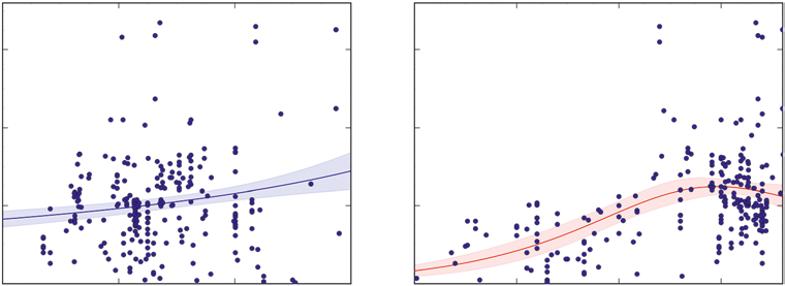
The graphs in Figures B and C come from a massive dataset for tropical forests around the world. Taylor et al. (2017) compiled information on rates of wood growth, with basic information on each location’s annual precipitation and average temperature (this example shows up again in Chapter 2). We know that trees need large amounts of water, because water evaporates (transpires) from leaves as the leaves absorb carbon dioxide from the air. We might have an idea that forests with a higher water supply should grow faster. This idea may or may not be true for forests, so checking the evidence from many studies lets us determine if this idea is worthy of our confidence. Indeed, forests with the highest amounts of precipitation grew more stemwood than those with a moderate supply. A few key features are worth pointing out. The X axis for precipitation spans a sevenfold range, from 1000–6000 mm yr−1. The Y axis for stem growth also spans a large range, but the line in the graph goes only from a bit more than 4 Mg ha−1 yr−1 to something less than 8 Mg ha−1 yr−1. Note that a sixfold change in the X axis (precipitation) gives at most a twofold range in stem growth, so the response is not as dramatic as if a twofold difference in precipitation gave a sixfold change in stem growth. Water matters, but not as much as we might have expected.
A second point for the first graph is that the average across all the studies follows a simple trend: a given increase in precipitation gives about the same amount of increase in stem growth, regardless of whether we look at the dry end or the wet end of the spectrum. We might have guessed that a small increase in water for dry sites would have a bigger value for tree growth than the same increase on a site that is already wet, but the available evidence would not support that generalization.
FIGURE B Stem growth in tropical forests is higher for sites with higher precipitation (left). The association with temperature is more complex, increasing at low temperatures and declining at the highest temperatures (Source: from data in Taylor et al. 2017).
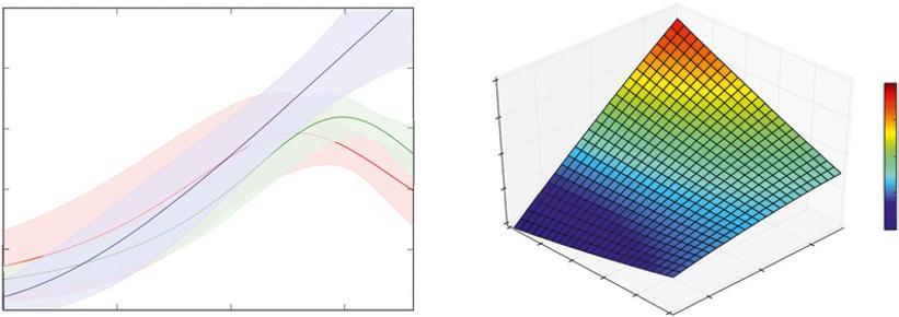
FIGURE C The influence of both factors can be examined together by examining the response of growth to temperature for three precipitation groupings (lower left). Putting sites into precipitation groups leaves out some of the information in the full dataset, and a 3D graph makes use of all the information. 3D graphs can work well for illustrating the overall trend surface, but specific details may be easier to read on 2D graphs (Source: from the database compiled by Taylor et al. 2017).
Just because the line in a graph goes up does not mean the trend warrants high confidence. If we chose a set of three numbers at random, the odds are good that the average trend would go up or down, rather than be flat. But if we choose a set with 100 random numbers, the odds are very high indeed that the trend would be flat (as there was no chance of the value of Y being related to X). This third point is illustrated with the shaded band around the line in the first graph, which represents the 95% confidence interval around the line. This means the evidence says the true trend would fall within that band about 95% of the time if the sampling were repeated. If we plotted a line with 240 random points for stem growth for random levels of precipitation, the line would be close to flat. If a flat line was placed into Figure B, it would fall outside the shaded bands of the confidence interval, so high confidence is warranted that sites with high rates of forest growth also tend to have higher precipitation. The odds are less than one in one thousand that growth and precipitation are unrelated (a flat line; this is the “P” value in statistics, which was <0.001 for this trend). This relationship of course does not prove that having more water is the key to producing more growth, but it does show the idea is not counter to the available evidence.
A third point about the first graph is that the dispersion of points around the line is broad indeed. Two tropical forests that have the same amount of precipitation might easily differ by twofold in growth rates. Even if confidence had been warranted in an average effect of precipitation, the average trend would not give a strong prediction for any single observation: half of all observations are always above average, and half below, no matter how much confidence is warranted in the overall trend.
This dispersion of points around the average trend is the fourth important story in the first graph. In statistics, the dispersion is the variance of the sample, and a number is often applied to trends in graphs that characterizes this dispersion around the
average. The correlation coefficient (r) describes how tightly the data clump near the average trend, and the square of the correlation coefficient (r2) tells the proportion of all the variability in Y values that relates to the level of the X values. In the first graph, the r2 for stem growth in relation to precipitation is 0.04 (4%). We can be strongly confident that stem growth on average increases with precipitation, but that knowledge accounts for only a very small part of the full distribution of growth rates of tropical forests. The idea seems likely to be true, but it gives very little power for precise predictions.
The second graph in Figure B shows the growth rates of the same forests, but in relation to the average annual temperature. The confidence band is a bit tighter in this case, and the dispersion of points around the trend is not as large. The probability that random noise would account for the pattern is quite small (less than one in a thousand), so high confidence is warranted in the association between stem growth and temperature. The average trend with temperature accounts for about 23% of all the variation in growth rates among sites (r2 = 0.23). Does higher temperature directly cause higher growth rates of forests? Possibly, but the association between two things does not mean that one causes the other. It’s possible that soil nutrient supply is the real driver of growth, and soils in warmer parts of the Tropics have higher nutrient supplies. Confidence in whether one thing actually drives another depends on further evidence (and often direct experimentation).
The growth of a forest with a given temperature could depend on water supply. The range of sites could be divided into three groups: sites with less than 2000 mm yr−1, 2000–4000 mm yr−1, and more than 4000 mm yr−1 (Figure C). The trends between temperature and stem growth are similar across these three groups at temperatures below 23 °C, but at higher temperatures growth seemed to decline more on drier sites than on wetter sites. This breakdown of the temperature relationship into three precipitation groups increases that amount of variation accounted for in growth to 31%, and very high confidence is warranted that predictions of temperature responses of growth differ among the precipitation groups.
Separating the sites into precipitation groups actually throws away some information that might be useful. For example, a site with 1950 mm yr−1 precipitation would be tallied in the driest group, and one with 2050 mm yr−1 would be separated into the medium group. Yet these two sites would be more similar to each other than the 2050 mm yr−1 site would be to another in the medium group with 3950 mm yr−1 site. Another version of the analysis could be done with all the data from each site allowed to influence the trend, and then a full three-dimensional pattern can be developed. The second graph in Figure B has two horizontal axes. The temperature axis increases to the right, and “backward” into the 3D space. The precipitation axis goes the other way, increasing to the left and also going backward into the space. This graph shows how any given level of temperature, and any level of precipitation, connect to give an estimate of the expected rate of stem growth. Keeping all the information on precipitation included (rather than lumping into three groups) increases the variation accounted for to 34%. A key difference is that this full-information analysis shows that growth continues to increase at high temperatures if the precipitation is high, but levels off (with no decline) on drier sites. This might seem like a small improvement in the pattern, but the improvement does warrant very high confidence.
It can be challenging to read the values for stem growth on the 3D graph, compared with straightforward 2D graphs. The grid lines give some help for visualizing how the overall trend changes, and the use of colors helps peg a value to any given point on the surface. Overall, 3D graphs can be very useful for illustrating overall trends, but 2D graphs might be more useful when the precise values of variables need to be identified.
Why do temperature and precipitation relate to only about one-third of all the variation in stem growth among tropical forests? Two points are important. This analysis used only annual averages, and two sites with similar annual average might differ in important seasonal ways. A given amount of rain spread evenly across 12 months might have very different effects on growth than if all the rain fell during a 4-month rainy season (with no rain for 8 months). The second point is that stem growth depends on a wide range of ecological factors, including soil nutrient supplies, and the genotypes of trees present. Attempts to explain forest growth often go beyond the ability of graphs to capture the relationship, using simulation models and other tools that have a chance to capture variations in growth patterns that go beyond two or three dimensions (Chapter 7).
The Most Important Points to Understand from Figures B and C Are Not About Precipitation or Temperature
The most important point is one that is not found in the graph, but applies to this graph and most others in this book. Graphs plot the values for a variable (such as forest growth) based on another variable (such as precipitation). Even when the association between the two variables is very strong, it’s fundamentally important to recognize that evidence of an association is not evidence of a cause-and-effect relationship. The forests that provided the data for Figure B had very different species composition, different soils, different ages, and different local histories of events. Some of these may happen to vary with precipitation, and might be the actual drivers of the trends that relate to precipitation. Similarly, if forest growth tended to decline in the warmest sites, that might result from increased activities of insects (or monkeys) rather than a direct effect of temperature.
Identification of driving causes behind patterns requires other sorts of evidence, especially evidence from experiments. If the addition (or removal) of water changed growth as much as was expected from the geographic gradient, then increased confidence would be warranted in water influencing growth across many locations. If plantations of a single species also declined in growth at high temperatures, then the trend in Figure B may be less influenced by changes in tree species across sites.
This fundamental idea is summarized in the aphorism, “Correlation does not equal causation.” All scientists know this, but placing science into sentences can be challenging for both thinking processes and writing processes. It’s easy to find examples where scientists forgot this basic point (perhaps even a few places in this book?).
Confidence Bands Around Trends Come in Two Types
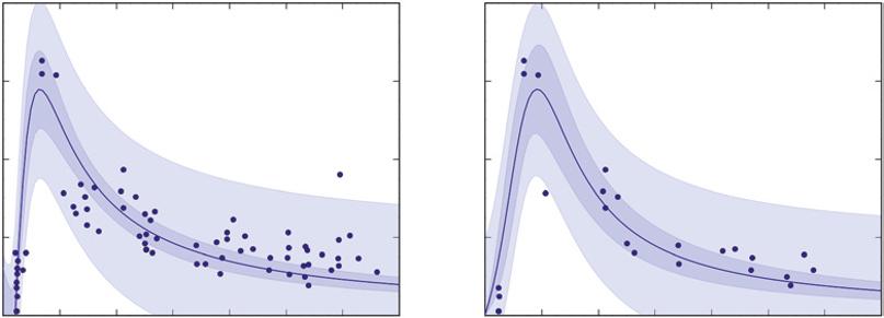
Most of this book’s graphs have shaded bands around the trend lines, and these represent the 95% confidence interval around the trend. A narrow band means the value on the Y axis was tightly related to the value on the X axis. Other types of bands can also be used, and Figure D shows a band that describes the distribution pattern for all the observations rather than the confidence warranted in the average trend. Both shaded bands in Figure D deal with 95%, but one describes the region where 95% of the observations are likely to be found, and the other the region where 95% of the trends (from repeated experiments) would be expected to occur. A key point is that the variation in the population of forests does not depend on how many samples are taken; a given proportion of forest would be a bit smaller (or much smaller) than average, and another proportion would be a bit larger (or much larger) than average. That variation does not change as the number of forests are sampled from the same landscape of forests. A sample of 24 forests produces about the same light-shaded band as a sample of 71 forests, but the confidence warranted in the trend is tighter when based on a larger number of samples (the dark bands).
The Stories in This Book Have Two Pieces, Told in Three Ways
The subject of forest ecology combines two different types of pieces: information (or evidence) about important details, and frameworks for how to knit pieces of information into understanding how forests work. The framework described above repeats throughout the book, along with many case studies and experiments that fill in information. This two-piece approach shows up in three complementary ways. The section headings state the key points in each chapter; these headings could be grouped together for
Based on plots from 71 forests
Based on plots from 24 forests
FIGURE D Rates of wood growth for lodgepole pine forests in Yellowstone National Park, Wyoming, USA rise quickly as new forests develop after fires, and then decline more slowly. The left graph shows that confidence in the average trend is warranted within the dark 95% confidence band. The points are dispersed around that average trend, and the lighter band covers the domain where about 95% of the observations would occur. The graph on the right used only a subset of 24 of the plots, and the average trend is similar, but the smaller number of sampled stands leads to a wider 95% confidence band (the darker band) for the trend compared to the full dataset on the left. The light blue band represents where 95% of the observations would be expected to fall, and the breadth of that band is quite similar between the two sampling intensities (Source: based on data from Kashian et al. 2013; see also Figure 9.11). Larger numbers of samples reduce the uncertainty about average trends, but not about the level of variability among forests across a landscape.
a simple overview for each chapter. The text of each chapter lays out the information and framework in detail, while the figures reinforce the headings and text with a third dimension of images and graphs (with detailed captions). Each of these three ways contributes to understanding forest ecology, developing a foundation to be built upon with further conversations, with readings of other books and journals, and especially with curious explorations in forests and across landscapes.
Forests Are Complex Systems That Are Not Tightly Determined
A core idea in this book is that forests are indescribably complex systems, with an uncountable number of interacting pieces under the influence of external driving factors. Simple stories cannot provide high value for specific cases, because the future development of a forest simply is not constrained enough to allow precise predictions. The good news is that evidence from thousands of research investigations around the world does provide a foundation for useful general insights. The next step is to apply general questions – from the core framework and core methods – to any forest of interest to develop strong, locally relevant knowledge. This book tries to clarify some of the basic nature of forests, and how to rely on evidence as a guide for gauging the amount of confidence warranted in ideas about forests.
A different forest ecology book could be written to summarize what we know about the major features of forests: for a very wide variety of questions, what solid answers emerge for each question from the evidence accumulated over the decades and centuries? That approach would provide a strong reference source for describing the general trends for forests, how variable they are, and what factors account for when forests are likely to be above or below the general trends. The focus of this book is somewhat different, though, as it fosters the thinking and understanding that will provide a strong foundation for adding later evidence found in reference books, journals, and other sources.
The future is not yet written for any forest, and that’s also true about this book. If revised editions should appear in the future, they would be much improved by feedback provided by readers of this edition. I gratefully invite feedback about typos, mistakes, omissions, and ideas for how the stories could be stronger and warrant more confidence (Dan.Binkley@alumni.ubc.ca).
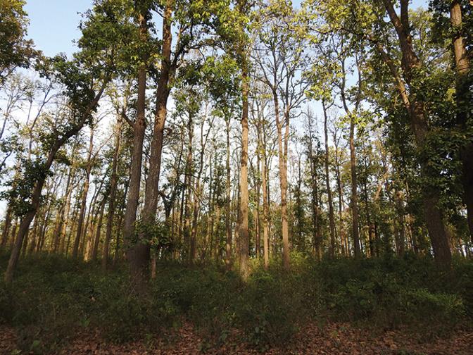
The final introductory point is that this book could be rewritten with all of the graphs and all of the examples switched out with different examples from other forests in other locations and other times. For example, sal (Shorea robusta) is a major, important tree in forests across southern Asia (Figure E), but this is the only sentence in the book that mentions sal. Each reader can make use of the book’s questions and perspectives by adding local information for other forests types, other places, and other times.
FIGURE E Sal is a major species across southern Asia, just one species of 700 among 16 genera in the Dipterocarp family. Sal wood is valued for lumber, its leaves are used for various purposes (including plates for food), and oil extracted from its seeds are used in food and mechanical applications (Source: photo by Anand Osuri).
Acknowledgements
It takes a virtual village to write a book, and I want to acknowledge and thank the villagers whose insights shaped this book, and my career. Each of my university advisors contributed new dimensions to thinking about forest ecology. Wally Covington at Northern Arizona University set the stage, and brought out interests in connecting chemistry and ecology. Hamish Kimmins at the University of British Columbia broadened my experiences, and patiently endured my skeptical challenges of so many ideas. Kermit Cromack’s curiosity and enthusiasm across a broad range of ecology and science was infectious – and persistent. Ed Packee at MacMillan Bloedel provided the questions, insights, funding and free reign that were so important early in my career. Colleagues and students at Duke University’s School of Forestry and Environmental Studies could not have done a better job of sustaining the momentum provided by earlier members of the village. The worldwide community of scientists in forest ecology and forest soils provided collaboration, ideas, and education over the following decades. Some of the most generous villagers were Tom Stohlgren, Mike Ryan, Peter Högberg, Bill Romme, Bob Powers, Dale Johnson, Jose Luiz Stape and Bob Stottlemyer. Most of my career developed at Colorado State University, with world-class colleagues and students. I cannot conceive of any village that would have been more fun, more supportive, or more productive; this tree acknowledges coauthors across four decades, with font sizes proportional to how many works we wrote together. Thanks to all of you – and to Mason Carter and Jane Higgins for working through and polishing these chapters. There are many ways a forest ecology textbook could be written; this is the one I could write.
The Nature of Forests
To see a World in a Grain of Sand, And a Heaven in a Wild Flower, Hold Infinity in the palm of your hand, And Eternity in an hour.. . .
William Blake (1757–1827)
William Blake’s poetic approach of seeing the general in the specific is a useful approach, two centuries later, for launching into the ecology of forests. The biology of a single tree in a single hour connects outward in time to the course of the tree’s development from a seed, back through evolutionary time for the genes comprising the tree’s genome. The environmental influences on the tree also connect outward in space, with strong similarities to the forces shaping trees around the world. The value of this literary approach to describing and understanding forests has limits: trees comprise the greatest part of the living matter within a forest, but the vast majority of organisms and species in forests are not trees at all. The biodiversity of forests resides primarily in understory plants, animals, and especially very small organisms such as arthropods, fungi, and bacteria.
The ecology of forests can be explored using Blake’s approach of starting very small to begin to understand very large and complex systems. The hourly, daily, and annual story for a single tree can be expanded outward to encompass the other trees in a forest, a landscape, and the forest biome, just as an hour can be expanded to a day, a year, a millennium, and evolutionary timescales.
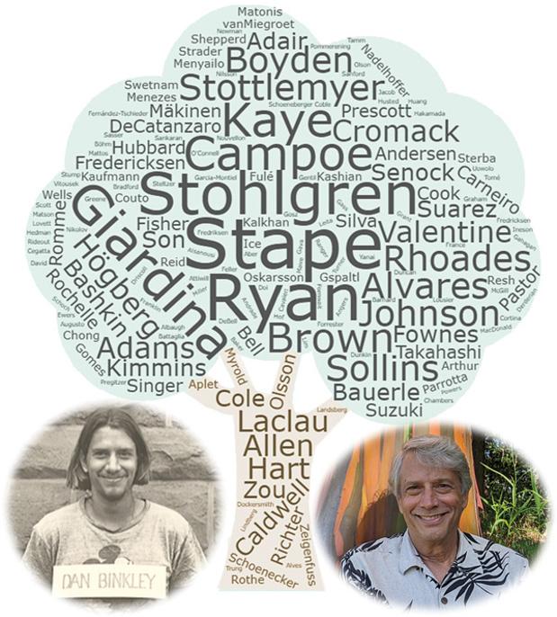
Forest Ecology Deals with Individual Trees Across Time
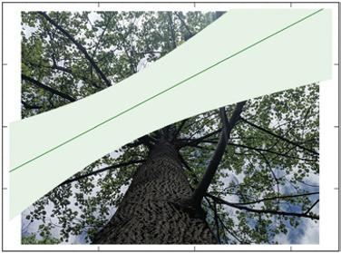
A tulip poplar in the Coweeta Basin of eastern North America will be the launching point for developing insights about forests. This particular tree (Figure 1.1) would be over half a meter in diameter (at a height of 1.4 m above the ground, a common point for measuring) and over 30 m tall. Eighty years of biological processes have led to an accumulation of more than 1000 kg of wood, bark, leaves, and roots. The actual living weight of the living tree would be about twice this mass of the biomass, because trees typically contain as much water as dry matter.
The crown carries about 75 000 leaves, with a total mass of about 25 kg (not counting the water). This is enough leaves to provide more than four distinct layers of leaves above the ground area below by the tree crown. The multiple layers of leaves are displayed to capture 90% of the incoming sunlight. A sunny afternoon might have 1000 W of sunlight reaching each m2 of ground area.
Many Processes Occur in a Tree Every Hour
Over the course of an hour, the tree leaves would intercept about 140 MJ of sunlight, and about half of the light arrives at wavelengths that can be used in photosynthesis. Perhaps 10–15% of the light reaching leaves reflects back into the environment, with no effect on the leaves. About one-third to one-half is converted to heat, warming the leaves, which then lose heat to the surrounding air (especially if the wind is blowing). Most of the rest of the intercepted energy is consumed as water evaporates from moist leaf interiors into the dry air, also cooling the leaves.
FIGURE 1.1 The Tree. This tulip poplar is a typical tree for temperate forests. The tree may live for a few centuries, integrating daily, seasonal, and yearly fluctuations in environmental conditions to turn carbon dioxide and water into wood (and thousands of types of chemicals).
A few percent of the radiant energy hitting leaves is harnessed to drive photosynthesis, producing about 30 g of sugar in this tulip poplar in an hour. The carbon contained in the newly formed sugar enters the leaves as carbon dioxide (CO2) during the same hour as the light interception. Small, adjustable openings (stomata) in the underside of the leaves allow CO2 to diffuse into the interior of the leaves as photosynthesis depletes the concentration of CO2 inside leaf cells. The rate of diffusion from the air into the leaf depends on the difference in concentration between CO2 in the atmosphere and inside the leaf. The air has about six times the concentration of CO2 that would be found inside photosynthesizing leaves, providing a steep gradient for the movement into the leaves. The remarkable biochemical processes in the leaves depend on the presence of more than a dozen elements in the tree, including 500 g of nitrogen (N) and 50 g of phosphorus (P). The bulk of these nutrients were taken up from the soil earlier in the season, but a sizable portion came from reserves that were recycled from last year’s leaves and stored over winter in the wood.
The 30 g of sugar produced during an hour would be associated with a release of about 30 g of oxygen (O2), as oxygen is released when water is split as part of photosynthesis. It may seem that this oxygen could be an important source of oxygen for the atmosphere, but it isn’t. As with all accounting in ecology, half a picture might lead to the wrong conclusion. The sugar produced by the tree may be “respired” fairly soon to support the growth of new cells or to maintain old cells, and oxygen is consumed (reforming water) in this reaction. Some of the sugar ends up in longer-lived cells, but even these tend to be oxidized back to CO2 over years or centuries. Unless the carbon content of a forest increases across generations of trees, the generation of oxygen in photosynthesis is matched by consumption during respiration and decomposition, leaving no extra oxygen in the atmosphere.
Some of the sugar produced by photosynthesis is consumed within the leaf to produce and support the metabolic needs of cells in the leaf. More than three-quarters of the sugar is loaded into the phloem and sent to flowers, twigs, branches, stems, roots and symbiotic root fungi (mycorrhizae).
Exposing the moist interiors of leaves to the dry air allows for uptake of CO2, but also allows water to be pulled into the dry air. The production of one molecule of sugar entails an unavoidable loss of hundreds of molecules of water. The production of 30 g of sugar in an hour would be accompanied by a far greater loss of water, perhaps 10 liters (10 kg) of water. The water transpired by the leaves during an hour of photosynthesis would have been found lurking in the soil a day earlier, and may have been in the atmosphere a day or a week before.
The tree has tremendous surface area developed within the soil to facilitate uptake of water and nutrients. The surface area of fine roots may be in the order of 100 times the surface area of leaves in the crown, and the surface area of mycorrhizal fungi that colonize roots contribute more than 10 times the surface area of roots. This vast surface area of absorbing roots and fungal mycelia collects water (and nutrients) that move up through the sapwood of the tree. The sapwood is comprised of xylem vessels, each measuring about 0.1 mm in diameter by 1 mm in length. The water passes through more than 1000 vessels for every meter of tree height, taking half a day or a day to move from all the way from roots to leaves.
Lifting water from the soil to the crown requires energy to overcome gravity, about 300 J for 10 liters. This is a tiny amount of energy compared to energy consumed as liquid water in leaves becomes water vapor in the atmosphere (about 2400 kJ for each liter, or 24 MJ for 10 liters). All the energy consumption and dissipation by the tree crown result in a deep shade beneath the tree. The air temperature in the shade may be a degree or two cooler than the air above the crown, but the shade will feel much cooler to a person sitting under the tree because of the greatly reduced energy load from the incoming sunlight.
Tree Physiology Follows Daily Cycles
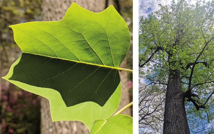
Over the course of a day, the tulip poplar responds to the changing environment through a daily cycle just as strongly as an animal would. The uptake of CO2 (and loss of water) begins as the sky brightens across the hillside in the morning, increasing as the intensity of sunlight increases (Figure 1.2). Rates may be highest near noon, decreasing if clouds develop, or if the air becomes so dry that the tree tightens the stomata to avoid losing too much water. Increasing temperatures in the afternoon drive up the capacity of air to hold water, resulting in a climb in the vapor pressure deficit. This deficit is a key force driving the water use by the tree. The tulip poplar would produce about 250 g of sugar on a sunny summer day (more than the average mentioned above for all days of the growing season), when the soil was moist, and transpiration could total 70 liters of water.
Not all processes in the tree shut down when the sun sets. Chemical reactions inside cells continue to renew thousands of biochemicals, generating and expanding new cells, and actively absorbing nutrient ions (such as nitrate and phosphate) from the soil. All of these processes require energy, most of which is supplied directly or indirectly from the sugars formed by photosynthesis. The oxidation of the sugar leads to substantial release of CO2 from the tree; this “respiration” in all the tissues of a tree may equal half of the total photosynthesis that occurs on a sunny day.
FIGURE 1.2 The daily pattern of incoming sunlight (A) reflects the geometry of the Earth’s tilt, the aspect and slope of a hillside, and the passing of clouds through the day. Temperature patterns (B) are driven in part by incoming sunlight, moderated by winds and evaporation of water (which cools the air). The combination of temperature patterns determines the capacity of air to hold water, and the vapor pressure deficit (C) tracks the difference between the current humidity of the air and the saturation point of the air. All these factors influence the rate of water use by the tulip poplar (D), though the connection to vapor pressure deficit is the most direct. Source: Data from Chelcy Miniat.
Trees Must Cope with Seasonal Cycles Through Each Year
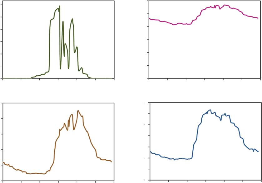
The environment surrounding the tulip poplar changes through the course of a year. The daily cycles of temperature swing between 5 and 10 °C, while the coldest and warmest day of the year may differ by 25 °C or more (Figure 1.3). Incoming sunlight in winter averages about half the level experienced in summer, as a result of shorter days, lower sun angles, and fewer clouds. These environmental changes lead to regular, predictable patterns in the phenology of the tree.
The tulip poplar begins an annual cycle of flowering and growth with the initiation of root growth late in the winter, followed by flowering in April and May. The tulip-shaped flowers are pollinated by bees and other insects, with 10 000 seeds raining from the crown in autumn. The leaves of the crown also expand in April and May, from expanding buds that were set the previous year. The initial burst of leaf growth depends on stored sugar, but the leaves rapidly provide new sugar for their own growth, and for the growth of all parts of the tree. The growth of a new leaf requires only about one-week’s production of sugar; the rest of the span of the leaf’s existence contributes to the growth and maintenance of other tissues.
Over the course of the growing season, the tulip poplar may produce 50 kg of sugar. Respiration would consume half, and the growth of short-lived roots and leaves might consume another quarter. Less than 25% of the annual production from the tree’s leaves would be found in new stem wood, increasing the diameter and height of the tree. The annual growth of the tree might use more than 8000 liters of water.
Dry periods during the summer lower the rate of photosynthesis in two ways. Low supplies of water in the soil lead to closure of leaf stomata, restricting both the gain of CO2 and the loss of water. The tulip poplar might also respond directly to the dryness of the atmosphere, and days with very high vapor pressure deficits may have low rates of photosynthesis, even if the soil is moist.
Trees Grow and Reproduce at Times Scales of a Century
Tulip poplar trees originate from seeds that develop following pollination of a flower by a bee or other insect. The flower may have developed on a parent tree as young as one or two decades, or as old as one or two centuries. Seeds develop over a period of five or six months, and then fall to the ground within a radius equal to a few times the height of the parent tree. A single seed
FIGURE 1.3 Seasonal trends in incoming sunlight (A) lead to almost twofold differences between summer and winter. The difference might be larger if not for the frequent cloud cover in summer. Patterns in incoming light lead to both daily and seasonal patterns in air temperatures (B). These environmental driving forces combine with the biology of the tulip poplar to determine the seasonal course of water use by the tree (C). Source: Data from Chelcy Miniat.
may germinate the following summer, or several summers later. The vast majority of seeds may never germinate, or if they germinate may not lead to a successfully established seedling. New seedlings require a great deal of luck to establish, including obtaining enough water and nutrients from the soil to support the development of leaves, and enough sunlight (perhaps 10% of full sun) to drive photosynthesis. The full intensity of sunlight may dry out a seedling, or overwhelm the photochemistry of new leaves.
A tulip poplar stem may not be the “first generation” of the “tree.”
A tree stem may die (from a wind storm breaking the stem, or a saw harvesting the tree), and a new stem may develop from dormant buds in the stump. The early growth and development of sprouted stems is faster and more assured than the tenuous development of a new seedling.
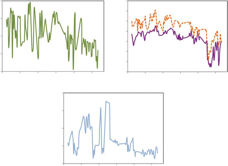
Weather differs a lot from one year to the next, and the growth of the tree during favorable periods may be double the growth rate for droughtier times (Figure 1.4). This response of an individual tree is the outcome of several factors, including the direct effects of the environment on this tree’s physiology, and the indirect effects of how fluctuations in the environment change the competition between trees in the forest.
FIGURE 1.4 Growth of yellow poplar trees is low in drier summers (a negative value for the Palmer Drought Severity index), and increases with increasing summer moisture. Source: Data from Kardol et al. 2010.
The tree is larger than its local neighbors, and this “dominance” provides a twofold advantage. The tree obtains a higher supply of light, water, and nutrients than its neighbors, driving faster growth. Faster growth then leads to a positive feedback that increases the tree’s capture of resources, allowing its growth to increase at the expense of neighbors.
The Story of Forests Is More than the Sum of the Individual Trees, Because Interactions Are So Strong
The tulip poplar tree is enmeshed in a complex ecological system (Figure 1.5). The tree provides habitat for an intricate community of insects and other arthropods. Each kilogram of leaves supports a total arthropod community of about 1 g (Schowalter and Crossley 1988), so the total leaf mass of the crown of 25 kg would support about 25 g of arthropods. Some of these invertebrates feed on the tree, eating leaves (or the insides of leaves), sucking sap, and boring into the wood of branches and the stem. Occasionally the populations of tree-feeding insects might increase to the point where much of the forest canopy is eaten; in most cases trees survive defoliation by native insect herbivores and form new canopies in the same season. Forests have other arthropods that feed on the species that feed on trees, forming complex food webs that include small mammals, a dozen or more species of birds, and even fish in streams and ponds that feed on arthropods from within the forests.
Does the tree benefit from neighbors, or is competition for resources the major effect of neighbors? Competition between trees is very important in all forests, but some possibilities exist for interactions between trees that actually benefit neighbors. One example is having a nitrogen-fixing black locust tree as a neighbor. The tulip poplar would compete with the locust for light, water, and other nutrients, but it might benefit from the enrichment of the soil N supply by the locust. Dozens of species of plants in the understory also compete with overstory trees for soil water and nutrients.
The diversity of plant species may be impressive, but this diversity is overshadowed by the diversity of invertebrates. Each square meter of soil contains about 60 large invertebrates with a total mass of about 1 g (Seastedt and
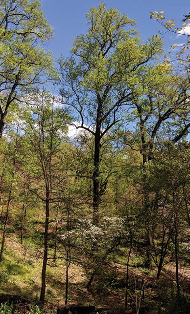
The dominant tulip poplar tree in the center of this springtime photo is part of a complex ecological system that includes other tulip poplars, other trees from more than a dozen species, several dozen species of understory plants, hundreds of species of arthropods and other invertebrates, and a soil that is itself a complex system with a level of biodiversity that dwarfs the diversity of the rest of the forest.
FIGURE 1.5
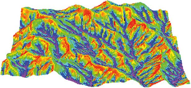
FIGURE 1.6 Although this looks like a topographic map of the Coweeta Basin, the colors actually represent the amount of water available for use by trees (hot colors are droughty sites, cool colors are wetter sites), and for draining into streams. Higher elevations receive more rainfall (and snow) than lower elevations, but water also flows downslope through soils, enriching lower parts of landscapes. Source: Map provided by D.L. Urban.
Crossley 1988). The number of small invertebrates would be on the order of 10 000 individuals (from hundreds of species) in each square meter; most of these feed on soil fungi.
Each kg of the upper mineral soil contains about 1 or 2 g of fungi, bacteria, and Archaea (Wright and Coleman 2000). The microorganisms are responsible for the majority of the processing of dead plant materials, returning carbon dioxide to the atmosphere, releasing inorganic nutrients into the soil, and altering soil structure and aggregation in ways that protect some organic matter from decomposition for decades, centuries, and even millennia. The small size of the soil microorganisms is matched by an almost unimaginable diversity of “species” or taxonomic units (as the concept of species does not apply well to many microbes). A 10 m by 10 m patch of soil likely contains more than 1000 species (or taxonomic units) of Archaea, another 1000 species of fungi, more than 10 000 species of bacteria, and 10 000 varieties of viruses (Fierer et al. 2007). This biocomplexity remains a largely unexplored frontier in the ecology of forests.
No two locations in the Coweeta Basin have exactly the same forest structure and composition, because local details (such as small variations in soils, or legacy of historical events) always shape local forests. Some broad forest patterns do repeat across the landscapes, as a result of patterns in topography. Precipitation increases by about 5% with each 100 m increase in elevation, rising from about 1500 mm yr−1 at 700 m elevation to more than 2200 mm yr−1 at 1500 m. Local topography modifies this elevational pattern, as wind flow near ridges can lead to 30% less precipitation falling below the ridgelines than would be expected based on elevation alone (Swift et al. 1988). The water available for use by trees (and flow into streams) depends heavily on local topography. Forests on ridgelines receive water from precipitation, and lose water through evaporation, transpiration by plants, and seepage downhill. Forests lower on the landscape receive water not only as precipitation, but also as water draining from higher slopes. Although more rain falls at higher elevations at Coweeta, some forests at lower elevations have access to more water because of this downhill flow (Figure 1.6).
Temperature also changes with elevation, falling by about 0.5 °C for every 100 m gain in elevation; moist air shows less temperature change with elevation than dry air. The landscape pattern in temperature is also strongly influenced by slope and aspect; the amount of incoming sunlight can vary by more than a factor of two from south-facing slopes to north-facing slopes, generating temperature differences of several degrees. Steep slopes receive more light than flat areas if the aspect points toward the sun, or less light if the aspect faces away from the sun.
These patterns in soil water, sunlight, and temperature lead to predictable patterns in forest structure and composition. Concave slopes (coves) have abundant supplies of water and deep soils, with large forests dominated by tulip poplar, black birch, and eastern hemlock. Dry ridges and convex slopes have smaller forests of oaks and pitch pine. Uniform slopes at lower elevations have mixed-deciduous forests dominated by white and red oaks, hickories, and nitrogen-fixing black locust. Uniform slopes at higher elevations are typically dominated by northern hardwood forests, with sugar maple, red oak, and beech.
Differences in species with elevation and topography also lead to differences in forest diversity and size. Lower elevation forests in the Coweeta Basin average about 18 tree species in a hectare, with diversity declining to about 14 tree species ha−1 at upper elevations (Figure 1.7). Diversity shows no trend with topography, as concave locations (coves) have about the same number of species ha−1 as convex (ridge) locations. The largest forests occur at middle elevations, and in concave locations.
FIGURE 1.7 Forest patterns commonly vary with elevation and with local topography. The number of tree species occurring in a hectare at Coweeta declines slightly with increasing elevation (upper left), whereas tree diversity shows no pattern among concave (cove) locations through to convex (ridge) locations (upper right). The basal area of trees tends to be highest at middle elevations (lower left), and in concave slope locations. Source: Data from Elliott 2008.
The Coweeta Forests Aren’t the Same as Two Centuries Ago
Forests with large, old trees may give an impression of an unchanging system that seem to be stable for decades and centuries. Some temperate forests may fit this image, but most are quite dynamic. If we could visit a forest before and after 50 years of changes occurred, we would likely find that many of the small trees had died (perhaps replaced by others), along with some of the medium- and large-size trees. The overall size of the forest, in terms of height or mass of wood in living trees, may have increased, but typically this increase in the size of larger trees comes in part at the expense of smaller trees that died.
Forests also change more rapidly, as a result of rapid events that alter the typical year-to-year progression of changes. The forests at Coweeta experienced massive changes in the past two centuries (Figure 1.8) as a result of direct human impacts and unintended, indirect impacts.
The most noticeable change in the forests in the Coweeta Basin is the loss of the formerly dominant tree species, American chestnut. Long-lived, large chestnut trees were the most notable part of the forest in 1900. About half the trees in the forest were chestnuts, and chestnuts comprised about half of the forest biomass. An exotic fungal disease from Asia, chestnut blight, killed almost all the mature chestnuts in forests of eastern North America within a few decades. Not all the mature trees were killed outright, as the fungus creates a canker on the stem that topples the tree. Surviving root systems continue to send up hopeful shoots, but these also form cankers when the stems are few meters tall.
What did the demise of chestnut mean for the forest? Given that competition is so important in the interactions among trees, the loss of chestnut led to a dramatic increase in the biomass of other species, particularly oaks, red maple, and tulip poplar. These species responded not by increasing the number of trees in the forest, but with accelerated growth of the already-present stems.
American chestnut 1935 1990
Oaks
Red maple
Hickories
Dogwood
Yellow poplar
Tupelo
Witch hazel
Sourwood
Black locust
Birch
Pitch pine
Eastern hemlock
FIGURE 1.8 Forest composition in the Coweeta Basin in 1935 and in 1990. The total density of trees (left) declined from 3000 trees ha−1 to 1200 trees ha −1, while basal area (right) increased slightly from 27 to 28 m2 ha−1. The decline in tree density is a common feature of growing forests; as dominant trees increase in size, many smaller trees die. However, the trend in this forest was largely influenced by the drastic decline of chestnut. This formerly dominant species was decimated by the exotic chestnut blight disease. Source: Data from Elliott 2008.
Another major event reshaped parts of the forests of Coweeta after the vegetation survey in 1990 summarized in Figure 1.8. Before this time, eastern hemlock was a major tree species in wetter locations, such as coves and valley bottoms. The hemlock woolly adelgid is an exotic, invasive insect that has killed most of the eastern hemlocks across much of eastern North America. About half the hemlocks died within the first 5 years of the adelgid’s arrival (Ford et al. 2012), with 90% or more dead after 15 years (Ford et al. 2012; Abella 2018). The loss of large hemlocks led to drops in the number of trees in the forests by about half, and long-term changes may include expansion of both trees of other species and understory woody plants (such as rhododendrons).
Continuing back in time, the most notable event of the nineteenth century was the extinction of the passenger pigeon. This large (30 cm) bird was a major consumer of large tree nuts, including acorns, beechnuts, and chestnuts (Halliday 1980; Johnson et al. 2010). Huge flocks contained tens of thousands (perhaps even millions) of birds, with large impacts on dispersal of tree seeds and nutrient cycling (with concentrated feces beneath favored roost and nest trees). Passenger pigeons were the most dominant species of bird in eastern North America, and perhaps the most numerous bird species in the world. Over the course of a few decades, this species spiraled to extinction as a result of massive hunting, and perhaps the effects of changing forest cover and even exotic diseases. How did the forests change in the absence of passenger pigeons? This important question is easily asked, but probably cannot be answered without stronger historical records.
Two other human-related events marked the 1800s in the Coweeta Basin. The second half of the century saw Euroamerican settlers occupying the land. Their major impacts included some logging, agricultural cropping on a few hundred hectares, widespread grazing of pigs and cattle, and hunting of wildlife for food. The prior inhabitants were Cherokee Indians, forcibly removed in the 1830s. Cherokee influences on the forests included some agriculture (maize, squash, and beans), extensive hunting (primarily deer, turkeys, and bears); food collection (including tree nuts); and frequent use of fire to clear the forest understory (Van Derwarker and Detwiler 2000; Gragson and Bolstad 2006).
Across Dozens of Generations of Trees, Almost Everything
Changed at Coweeta
The past 10 000 years have seen dozens of generations of trees and forests come and go in the Coweeta Basin, in response to fluctuations in climate, events such as hurricanes, and probably sizable fluctuations in populations of humans and other animal species that influence forest dynamics. The frequency of fires may have increased as people ignited forest fires (intentionally or unintentionally). Fires may have burned the tulip poplar/mixed broadleaf stands every 200 years or so over the millennium before European settlement (Fesenmeyer and Christensen 2010). Some notable events include a near-disappearance of eastern hemlock throughout its range, between about 5500 and 6500 years ago (Calcote 2003; Heard and Valente 2009), followed by recovery. The cause of the decline is unknown, and speculations include some sort of novel disease. This also happened to be one of the coolest times in the past 10 000 years, so multiple factors may have been involved.
Continuing back to 12 500 years ago, the continent (and much of the globe) was undergoing rapid warming as the most recent Ice Age ended. Temperatures in the Coweeta Basin would have risen by more than 5 °C from conditions that prevailed for 100 000 years. Under colder conditions, the forests in the Basin would have resembled forests that are currently found farther north, with pines and spruces dominating even the lower elevations. During some periods, the assemblages of trees species across the region included combinations that have no modern analog in local forests, or in forests now found farther north (Jackson and Williams 2004). Assemblages of tree species change in response to interactions among temperature, precipitation, and biotic factors. Unlike organisms, the genotypes of forests change routinely as species come and go.
The most notable difference in the forest at the end of the Ice Age would have been the presence of many large species of mammals in the region. The list of now-extinct species includes tree-browsing American mastodons; grass and tree-browsing Columbian mammoths; woody-plant browsing stag moose; tree-eating giant beavers more than 2 m in length; and large predators such as dire wolves, sabretooth cats, and massive short-faced bears. The now-extinct mammals would have been joined by at least one now-extinct tree species, Critchfield spruce (Jackson and Weng 1999).
The Futures of the Tree and the Forest Will Depend on Both Gradual, Predictable Changes and Contingent Events
The future is largely unpredictable for individual trees, but some predictions may have a high probability of coming true. The dominant situation enjoyed by the tulip poplar featured in this chapter would generally predict steady growth into the future. Growth might even increase as neighbors are suppressed. Dominant trees of this species may live for more than two centuries, and such a long lifespan provides opportunities for dispersing millions of seeds.
A long lifespan also increases the odds that the tree will experience rare weather events. For example, a severe drought with a probability of occurrence once in 100 years might severely challenge a tree’s survival. A tree that lives only about five decades would have a 60% chance of never experiencing a 100-year-magnitude drought (if weather is random), whereas a tree that lived two centuries would have an 87% probability of experiencing at least one 100-year drought.
A host of other future factors are more difficult to assign probabilities. The death of a neighboring tree may suddenly increase the supplies of resources available to this tree, or the falling neighbor may collide and uproot this tree as well. Lightning tends to kill large trees more often than smaller trees. Outbreaks of insect populations and fungal diseases influence the long-term development of many forests. The climate experienced by this tree (and its ancestors) may not continue into the future. Novel pests may arrive in the forest, as a result of widespread transport associated with world-wide travel by people and materials. The future of the tree may also depend very heavily on choices made by people; a large tulip poplar tree can be transformed into thousands of dollarsworth of furniture and other products.
Some changes in a forest tend to be cyclic, with repeating patterns of species and growth rates following major events. The major recolonizing species will have predictably high tolerance for full sunlight and rapid early growth, whereas trees that remain after two centuries will likely grow slowly and the community will include trees that thrive under shady conditions. Other changes are clearly not cyclic, and lead us to expect that the future forests in the Coweeta Basin will not be simple analogs of past forests (Jackson and Williams 2004). The development of forests responds to changes in climate, and climatic patterns (and the responses of trees and species to these patterns) have long legacies (Kardol et al. 2010). Changes in future climates may have modest effects on the forests compared to novel insects and diseases. The chestnut blight removed the dominant tree species from the Coweeta forests, and the hemlock wooly adelgid decimated the population of eastern hemlock trees. What will be the legacies of the loss of almost all the chestnuts and hemlocks trees from Coweeta’s forests? Might we be able to predict the response of surviving species to the disappearance of hemlock, based on the patterns from 6000 years ago when eastern hemlock experienced another decline, or will other factors (such as changing climate) limit the ability of the past to illuminate the future? We might speculate about how other species will take advantage of reduced competition from these species, but the actual impacts will include the ecological legacies of changes in soils and in animal communities. Forests often respond to more than one event; future forests develop from the combined legacies of historical events (such as losses and gains of species) in combination with current conditions. Warming climate, rising atmospheric concentrations of carbon dioxide, and other factors will influence future forests, shaping the legacies of the losses of chestnuts and hemlocks. Will new species of exotic insects arrive and remove other tree species from Coweeta’s forests?
The future development of a tree, and of a forest, derives from the gradual accumulation of routine changes, such as annual increases in height and mass of stems. Over limited periods, these gradual, expected trends are punctuated by contingent events that are largely unpredictable, such as hurricanes and invasions by exotic pathogens. Humans are another force for change in forests, through direct management (typically favoring some species over others, often limiting the opportunity for old trees to develop) and indirect activities (such as nutrient enrichment of rain, air pollution, and climate change).
Given all these forces of change, how can we predict future forests? The short answer is simply that we cannot predict future forests with much confidence. The longer (and more useful) answer is that we can indeed develop insights about the likely forests of the future, if we understand some of the basic features that have shaped forests in the past, and how ecological interactions will combine to shape future forest.
Ecological Afterthoughts: Is a Forest an Organism?
A variety of traits and processes characterize all organisms: they process high-energy sources from the environment (such as sunlight or organic compounds) into low-energy byproducts (such as heat), and they grow, reproduce, and die. Forests do these same things. So are forests like organisms? We have a strong tendency for using analogies to make sense of the world, and sometimes we go beyond analogies to use metaphors, where one is not simply like another, but is essentially the same. Ideas about forests have arisen commonly from analogies, and sometimes even from metaphors. For example, an influential ecologist asserted a forests-areorganisms metaphor a century ago:
The unit of vegetation, the climax formation, is an organic entity. As an organism, the formation arises, grows, matures and dies. . . The life-history of a formation is a complex but definite process, comparable in its chief features with the life-history of an individual plant. . . Succession is the process of reproduction of a formation, and this reproductive process can no more fail to terminate in the adult form than it can in the case of the individual.
(Clements 1916)
Our ideas about forests can shape what we can see in forests, and the belief in the organism-nature of ecosystems led this ecologist to strong confidence in untested ideas, simply because he was seduced by the beauty of the organism metaphor:
It can still be confidently affirmed that stabilization is the universal tendency of all vegetation under the ruling climate, and that climaxes are characterized by a high degree of stability when reckoned in thousands or even millions of years.
(Clements 1936)
A metaphor that was true might be very useful, but a poor metaphor may be useless or even harmful. An untested metaphor could be a good starting point for science, but could not be a reliable conclusion. If forests were the same as organisms, the future composition, structure and function of forests would be largely predictable. Any deviations in that progression would risk the continued persistence of the forest. If forests are quite unlike organisms, such a belief would befuddle our ability to see the forest and the trees.
The “ecological afterthoughts” in later chapters are open-ended invitations to apply ideas from the chapters to specific situations. The afterthoughts are not intended to convey information or answers, but just to raise questions. This first chapter goes a bit further, highlighting how the afterthoughts might be used for insights.
A listing of similarities and differences would immediately show this metaphor of “Forests are Organisms” would be weak at best, and maybe harmful if taken too seriously. Forests clearly differ from organisms in fundamental ways (Figure 1.9). A tulip poplar seed can only lead to a tulip poplar tree, with growth rates and forms that are shaped by environmental factors and the genes of the tree. A tulip poplar that deviated from normal structure and function would soon be a dead tulip poplar, with no chance to send more of its genes into future generations.
A forest that contains tulip poplar trees is much less constrained in its future development. Unlike organisms, forests routinely gain and lose genes as members of species enter and leave the forest; there is no single way for a forest to be, and no single path that must be followed if a landscape will remain dominated by trees. If we believe forests are organisms, the loss of major components should be expected to endanger the whole. The death of an organism is an event that encompasses all its parts. The “death” of a forest is always a matter of perspective; major events kill some trees, plants and animals, leading to greater opportunities for the surviving trees, plants and animals. Forests persist through the gains and losses of individuals and species; organisms generally don’t persist through the gains and losses of organs (aside from seasonal senescence of leaves and fine roots). A tree that lost its leaves and never regrew a new set of leaves would die; a forest that lost all members of a given tree species (with that species never returning), would remain quite viable.
Several of the dominant species formerly found in tulip poplar forests disappeared from the landscape in recent times, including chestnut trees, passenger pigeons, wolves and mountain lions, while the human influences shifted from Cherokee to European cultures. Nevertheless, forests that contain tulip poplar trees continue to exist and change, as individual organisms and species shift in response to changing stresses and opportunities. The forests of the future will not be the same as those in the past, and change over time is a normal aspect of forests.
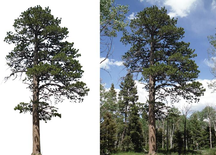
FIGURE 1.9 As with the tulip poplar and tulip poplar forest examined in this chapter, all trees have very limited scope in their development from seed to mature tree, and all forests have very broad scope in their composition and structure over time. This ponderosa pine tree (left) developed from a seed that contained genetic material from two parent trees. The potential future states of this plant were determined and constrained by these genes. The actual development of the tree depended on climate, weather events, fires, and interactions with a huge variety of microorganisms, animals, and other plants. No two ponderosa pine trees are identical, yet the range of differences among ponderosa pine trees is miniscule compared to the range differences in the composition of forests that contain ponderosa pine trees. Unlike the tree, the forest where this tree grew did not have a particular beginning; major events such as fires killed many trees, but many survived (including the root system of aspens that sent up a new generation of stems from ancient root stocks), as did many of the understory plants. The dynamics of the forest were not determined or constrained by the genes of a single species, and the composition of the forest shifted over the decades in response to climate, rapid events, and management. The forest continues as the death and birth of individuals subtracts and adds genetic possibilities for the future.
This flexibility in the genetic composition of forests ensures that the organism metaphor confuses rather than enlightens. Complex, changeable forests have far greater capacity for change than organisms, ensuring that the future development of forests is anything but precisely predictable.
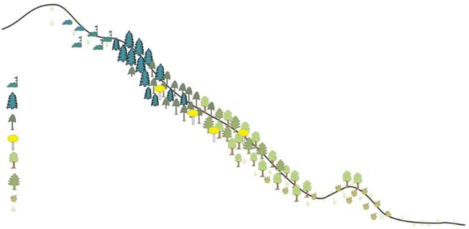
Forest Environments
Forests change across landscapes, and some of the changes result from gradients in environmental factors such as temperature and available water. Patterns of forest change across landscapes relate broadly to patterns of environmental factors, such as typical changes in the dominant species as elevation increases in mountains (Figure 2.1). Some broad generalizations may explain general patterns: temperatures are lower at higher elevations, and precipitation is generally (but not always) higher. The underlying details that influence both the broad patterns and specific cases are a bit complex and highly interacting. This chapter develops a foundation for understanding the fundamental physics that influence tree occurrence and growth. Later chapters expand to examine how ecological interactions (including plants, animals and microbes) and environmental factors combine to shape forests.
All the chemical and biological processes within a forest are driven by physical processes: environmental temperatures, water regimes, and solar radiation. In turn, the chemical and biological processing of solar energy shape the microenvironmental conditions found in forests. Interception of sunlight by trees not only drives photosynthesis, it leads to evaporation of water from leaves, cooling the leaf and increasing the humidity of the air. Evaporation of water from leaves (transpiration) physically lifts masses of water and nutrients from the soil up to the canopy, and cools leaves heated by sunshine. Energy “fixed” through photosynthesis cascades down a series of chemical reactions, driving the forest’s chemistry and biology until all the energy has been dissipated as heat. All the interesting biology and ecology that occur in forests take place within this physical system.
FIGURE 2.1 The vegetation in the Front Range of the Rocky Mountains in northern Colorado, USA grades from primarily grass/shrub domination at low, dry elevations, through open pine-dominated woodlands, to aspens mixed with a variety of conifers, to forests of spruce and fir and then to tundra (alpine) at the highest elevations (Source: based on a diagram from Laurie Huckaby). The patterns depend on direct effects of environmental factors on tree physiology, and also environmental influences on fires, insects, and other forest-shaping agents.