Semiconductor Basics
A Qualitative, Non-mathematical Explanation of How Semiconductors Work and How They Are Used
George Domingo Berkeley CA, USA
This edition first published 2020 © 2020 John Wiley & Sons Ltd
All rights reserved. No part of this publication may be reproduced, stored in a retrieval system, or transmitted, in any form or by any means, electronic, mechanical, photocopying, recording or otherwise, except as permitted by law. Advice on how to obtain permission to reuse material from this title is available at http://www.wiley.com/go/permissions.
The right of George Domingo to be identified as the author of this work has been asserted in accordance with law.
Registered Offices
John Wiley & Sons, Inc., 111 River Street, Hoboken, NJ 07030, USA
John Wiley & Sons Ltd, The Atrium, Southern Gate, Chichester, West Sussex, PO19 8SQ, UK
Editorial Office
The Atrium, Southern Gate, Chichester, West Sussex, PO19 8SQ, UK
For details of our global editorial offices, customer services, and more information about Wiley products visit us at www.wiley.com.
Wiley also publishes its books in a variety of electronic formats and by print-on-demand. Some content that appears in standard print versions of this book may not be available in other formats.
Limit of Liability/Disclaimer of Warranty
In view of ongoing research, equipment modifications, changes in governmental regulations, and the constant flow of information relating to the use of experimental reagents, equipment, and devices, the reader is urged to review and evaluate the information provided in the package insert or instructions for each chemical, piece of equipment, reagent, or device for, among other things, any changes in the instructions or indication of usage and for added warnings and precautions. While the publisher and authors have used their best efforts in preparing this work, they make no representations or warranties with respect to the accuracy or completeness of the contents of this work and specifically disclaim all warranties, including without limitation any implied warranties of merchantability or fitness for a particular purpose. No warranty may be created or extended by sales representatives, written sales materials or promotional statements for this work. The fact that an organization, website, or product is referred to in this work as a citation and/ or potential source of further information does not mean that the publisher and authors endorse the information or services the organization, website, or product may provide or recommendations it may make. This work is sold with the understanding that the publisher is not engaged in rendering professional services. The advice and strategies contained herein may not be suitable for your situation. You should consult with a specialist where appropriate. Further, readers should be aware that websites listed in this work may have changed or disappeared between when this work was written and when it is read. Neither the publisher nor authors shall be liable for any loss of profit or any other commercial damages, including but not limited to special, incidental, consequential, or other damages.
Library of Congress Cataloging-in-Publication Data
Names: Domingo, George, 1937– author.
Title: Semiconductor basics : a qualitative, non-mathematical explanation of how semiconductors work and how they are used / George Domingo, Berkeley, CA, US.
Description: First edition. | Hoboken, NJ, USA : Wiley, [2020] | Includes bibliographical references and index.
Identifiers: LCCN 2020015406 (print) | LCCN 2020015407 (ebook) | ISBN 9781119702306 (cloth) | ISBN 9781119597117 (adobe pdf) | ISBN 9781119597131 (epub)
Subjects: LCSH: Semiconductors. | Solid state electronics. | Electronic apparatus and appliances.
Classification: LCC TK7871.85 .D654 2020 (print) | LCC TK7871.85 (ebook) | DDC 621.3815/2–dc23
LC record available at https://lccn.loc.gov/2020015406
LC ebook record available at https://lccn.loc.gov/2020015407
Cover Design: Wiley
Cover Images: Computer motherboar © Bet_Noire/Getty Images, Two People - Drawn by Pey Llussà, Circuit Board © filo/Getty Images, Central processor unit © Artem_Egorov/Getty Images, Graphene sheet © KTSDESIGN/SCIENCE
PHOTO LIBRARY/Getty Images
Set in 9.5/12.5pt STIXTwoText by SPi Global, Pondicherry, India
Printed and bound by CPI Group (UK) Ltd, Croydon, CR0 4YY
10 9 8 7 6 5 4 3 2 1
To my family for their love and support
Contents
Acknowledgements xiii
Introduction xv
1 The Bohr Atom 1
Objectives of This Chapter 1
1.1 Sinusoidal Waves 1
1.2 The Case of the Missing Lines 3
1.3 The Strange Behavior of Spectra from Gases and Metals 4
1.4 The Classifications of Basic Elements 5
1.5 The Hydrogen Spectrum Lines 5
1.6 Light is a Particle 7
1.7 The Atom’s Structure 8
1.8 The Bohr Atom 10
1.9 Summary and Conclusions 13
Appendix 1.1 Some Details of the Bohr Model 14
Appendix 1.2 Semiconductor Materials 16
Appendix 1.3 Calculating the Rydberg Constant 16
2 Energy Bands 19
Objectives of This Chapter 19
2.1 Bringing Atoms Together 19
2.2 The Insulator 22
2.3 The Conductor 23
2.4 The Semiconductor 24
2.5 Digression: Water Analogy 27
2.6 The Mobility of Charges 27
2.7 Summary and Conclusions 28
Appendix 2.1 Energy Gap in Semiconductors 29
Appendix 2.2 Number of Electrons and the Fermi Function 29
3 Types of Semiconductors 35
Objectives of This Chapter 35
3.1 Semiconductor Materials 35
3.2 Short Summary of Semiconductor Materials 36
3.2.1 Silicon 36
3.2.2 Germanium 37
3.2.3 Gallium Arsenide 39
3.3 Intrinsic Semiconductors 39
3.4 Doped Semiconductors: n-Type 40
3.5 Doped Semiconductors: p-Type 43
3.6 Additional Considerations 45
3.7 Summary and Conclusions 47
Appendix 3.1 The Fermi Levels in Doped Semiconductors 48
Appendix 3.2 Why All Donor Electrons go to the Conduction Band 50
4 Infrared Detectors 51
Objectives of This Chapter 51
4.1 What is Infrared Radiation? 51
4.2 What Our Eyes Can See 54
4.3 Infrared Applications 55
4.4 Types of Infrared Radiation 58
4.5 Extrinsic Silicon Infrared Detectors 58
4.6 Intrinsic Infrared Detectors 62
4.7 Summary and Conclusions 63
Appendix 4.1 Light Diffraction 64
Appendix 4.2 Blackbody Radiation 66
5 The pn-Junction 69
Objectives of This Chapter 69
5.1 The pn-Junction 69
5.2 The Semiconductor Diode 72
5.3 The Schottky Diode 76
5.4 The Zener or Tunnel Diode 77
5.5 Summary and Conclusions 81
Appendix 5.1 Fermi Levels of a pn-Junction 81
Appendix 5.2 Diffusion and Drift Currents 82
Appendix 5.3 The Thickness of the Transition Region 83
Appendix 5.4 Work Function and the Schottky Diode 85
6 Other Electrical Components 89
Objectives of This Chapter 89
6.1 Voltage and Current 89
6.2 Resistance 90
6.3 The Capacitor 93
6.4 The Inductor 96
6.5 Sinusoidal Voltage 98
6.6 Inductor Applications 99
6.7 Summary and Conclusions 102
Appendix 6.1 Impedance and Phase Changes 102
7 Diode Applications 105
Objectives of This Chapter 105
7.1 Solar Cells 105
7.2 Rectifiers 106
7.3 Current Protection Circuit 109
7.4 Clamping Circuit 109
7.5 Voltage Clipper 110
7.6 Half-wave Voltage Doubler 111
7.7 Solar Cells Bypass Diodes 113
7.8 Applications of Schottky Diodes 113
7.9 Applications of Zener Diodes 114
7.10 Summary and Conclusions 115
Appendix 7.1 Calculation of the Current Through an RC Circuit 115
8 Transistors 117
Objectives of This Chapter 117
8.1 The Concept of the Transistor 117
8.2 The Bipolar Junction Transistor 118
8.3 The Junction Field-effect Transistor 124
8.4 The Metal Oxide Semiconductor FET 128
8.5 Summary and Conclusions 132
Appendix 8.1 Punch Trough 134
9 Transistor Biasing Circuits 135
Objectives of This Chapter 135
9.1 Introduction 135
9.2 Emitter Feedback Bias 136
9.3 Sinusoidal Operation of a Transistor with Emitter Bias 140
9.4 The Fixed Bias Circuit 144
9.5 The Collector Feedback Bias Circuit 147
9.6 Power Considerations 148
9.7 Multistage Transistor Amplifiers 149
9.8 Operational Amplifiers 150
9.9 The Ideal OpAmp 153
9.10 Summary and Conclusions 155
Appendix 9.1 Derivation of the Stability of the Collector Feedback Circuit 156
10 Integrated Circuit Fabrication 159
Objectives of This Chapter 159
10.1 The Basic Material 159
10.2 The Boule 160
10.2.1 The Czochralski Method 160
10.2.2 The Flow-zone Method 161
10.3 Wafers and Epitaxial Growth 162
10.4 Photolithography 162
10.5 The Fabrication of a pnp Transistor on a Silicon Wafer 163
10.6 A Digression on Doping 166
10.6.1 Thermal Diffusion 166
10.6.2 Implantation 167
10.7 Resume the Transistor Processing 170
10.7.1 The Contacts 170
10.7.2 Metallization 170
10.7.3 Multiple Interconnects 171
10.8 Fabrication of Other Components 172
10.8.1 The Integrated Resistor 172
10.8.2 The Integrated Capacitor 173
10.8.3 The Integrated Inductor 173
10.9 Testing and Packaging 174
10.10 Clean Rooms 178
10.11 Additional Thoughts About Processing 180
10.12 Summary and Conclusions 181
Appendix 10.1 Miller Indices in the Diamond Structure 183
11 Logic Circuits 187
Objectives of This Chapter 187
11.1 Boolean Algebra 187
11.2 Logic Symbols and Relay Circuits 188
11.3 The Electronics Inside the Symbols 190
11.3.1 Diode Implementation 191
11.3.2 CMOS Implementation 192
11.4 The Inverter or NOT Circuit 192
11.5 The NOR Circuit 193
11.6 The NAND Circuit 195
11.7 The XNOR or Exclusive NOR 196
11.8 The Half Adder 197
11.9 The Full Adder 198
11.10 Adding More than Two Digital Numbers 198
11.11 The Subtractor 199
11.12 Digression: Flip-flops, Latches, and Shifters 201
11.13 Multiplication and Division of Binary Numbers 203
11.14 Additional Comments: Speed and Power 204
11.15 Summary and Conclusions 206
Appendix 11.1 Algebraic Formulation of Logic Modules 206
Appendix 11.2 Detailed Analysis of the Full Adder 207
Appendix 11.3 Complementary Numbers 208
Appendix 11.4 Dividing Digital Numbers 209
Appendix 11.5 The Author’s Symbolic Logic Machine Using Relays 210
12 VLSI Components 211
Objectives of This Chapter 211
12.1 Multiplexers 211
12.2 Demultiplexers 213
12.3 Registers 214
12.4 Timing and Waveforms 216
12.5 Memories 218
12.5.1 Static Random-access Memory 219
12.5.2 Dynamic Random-access Memory 222
12.5.3 Read-only Memory 224
12.5.4 Programable Read-only Memory 225
12.6 Gate Arrays 227
12.7 Summary and Conclusions 227
Appendix 12.1 A NAND implementation of a 2 to 1 MUX 228
13 Optoelectronics 229
Objectives of This Chapter 229
13.1 Photoconductors 229
13.2 PIN Diodes 230
13.3 LASERs 231
13.3.1 Laser Action 231
13.3.2 Solid-state Lasers 234
13.3.3 Semiconductor LASERs 234
13.3.4 LASER Applications 237
13.4 Light-emitting Diodes 238
13.5 Summary and Conclusions 240
Appendix 13.1 The Detector Readout 240
14 Microprocessors and Modern Electronics 243
Objectives of This Chapter 243
14.1 The Computer 243
14.1.1 Computer Architecture 243
14.1.2 Memories 244
14.1.3 Input and Output Units 246
14.1.4 The Central Processing Unit 246
14.2 Microcontrollers 248
14.3 Liquid Crystal Displays 249
14.3.1 Liquid Crystal Materials 249
14.3.2 Contacts 251
14.3.3 Color Filters 251
14.3.4 Thin-film Transistors 251
14.3.5 The Glass 253
14.3.6 Polarizers 253
14.3.7 The Source of Light 254
14.3.8 The Entire Operation 254
14.4 Summary and Conclusions 255
Appendix 14.1 Keyboard Codes 256
15 The Future 257
Objectives of This Chapter 257
15.1 The Past 257
15.2 Problems with Silicon-based Technology 262
15.3 New Technologies 265
15.3.1 Nanotubes 265
15.3.2 Quantum Computing 266
15.3.3 Biocomputing 268
15.4 Silicon Technology Innovations 268
15.4.1 Process Improvements 269
15.4.2 Vertical Integration 269
15.4.3 The FinFET 271
15.4.4 The Tunnel FET 271
15.5 Summary and Conclusions 272
Epilogue 273
Appendix A Useful Constants 275
Appendix B Properties of Silicon 277
Appendix C List of Acronyms 279
Additional Reading and Sources 285
Index 289
Acknowledgements
I would like to recognize all those scientists, engineers, professors, authors, teachers, and also students who in the past 130 years with their research, experiments, theories, analysis, publications, and textbooks have been able to explain beautifully how matter behaves, how to use it, and how to explain it to the next generation of scientists. In the process they created an electronic revolution. As someone already said, we are sailing on the shoulders of all those thousands of geniuses that preceded us.
I want to acknowledge the efforts and support of the Wiley editors who made the text more readable and clearer.
I want to thank my family who have been always helpful, encouraging, and patient with me and my project.
Finally, I would like to mention Dr. Gerry Hanh, who upon reading the first chapters that I wrote as a hobby, insisted I send them to Wiley, resulting in the book you have now in your hands.
Introduction
A couple of years ago, I was asked to give a talk to the Rotary club in Terrassa, a city about 20 miles northwest of Barcelona. They asked me to divide the talk into three parts: 15 minutes biographical, 15 minutes on my technical work, and 15 minutes about NASA. The first and last 15 minutes of the talk went well, but the technical explanation about how infrared detectors work was disappointing. Yes, they did understand the uses and applications of infrared detectors, my technical work with the astronomical observatories of NASA, but the explanation on how infrared detectors work was not as clear and instructive as I had hoped. I was then and I am now convinced that any educated person can understand how semiconductor devices work. This talk two years ago was my motivation to start writing this book.
Semiconductors are the basis for almost all modern electronic devices. For many people semiconductors are a mysterious material that somehow has taken over modern electronics. In the same way that we understand the concept of god and creatures, but semi-gods are confusing, most of us have an idea of what a conductor (electricity flows through it) and an insulator (it doesn’t) are, but what the heck is a semiconductor? Furthermore, the prevalent material used for fabricating semiconductors is pure silicon, the second most common element found on earth (28%) after oxygen (47%). Why not use aluminum, the next common element (8%), or strontium or some other exotic and more classy material? Why do we use semiconductors instead of conductors? Don’t we want electrons to move freely through our devices?
I attempt here to explain why and how semiconductors work in a form that any educated person can understand. Every chapter explains the subject in a qualitative way, with drawings, photographs, and figures, and very simple relationships (I hate to use the word “equations” here). At the end of most chapters I add appendices where I include some mathematical formulation with the relevant equations for those who would enjoy looking a little deeper into the subject. I do not try to proof these equations; my purpose is not to formally present to you the physics of semiconductors (there are many excellent books that do that) but just to show what the results are. In this book you have to take these results on faith.
Unless you are very allergic to math, do not skip the appendices. There are interesting concepts that amplify the understanding of how semiconductors work. Don’t worry; there are no problems at the end of each chapter and no suggested quizzes.
First, I explain what a semiconductor is, the different types we use, and how they are different from conductors and insulators. Next, I explain the key devices that can be constructed using the semiconductor materials: diodes, passive element, and transistors. I talk about the integrated circuits, how we build them and the larger electronic components, and finally what can we expect in the future (Chapter 15). I interrupt the “theoretical” flow with chapters devoted to applications (Chapters 4, 7, and 9) that can be understood with just the concepts I have covered in the previous chapters.
This book can be read in different ways. If you are interested in understanding how transistors work, then you should read, in succession, Chapters 1, 2, 3, 5, and 8. You cannot skip any of them or read them in a different order unless, of course, you are already familiar with some of the previous topics. Chapter 6 explains the basic electrical components (resistors, capacitors, and inductors) which we need to understand how we build useful semiconductor circuits. I try to discuss some of the semiconductor applications as soon as I cover the relevant theory. Just by understanding the concept of energy levels and energy bands (Chapters 2 and 3) you can grasp how infrared detectors work (Chapter 4). You do not even need to know what resistors or capacitors are. Similarly, after Chapter 6 you can understand the different circuit applications we can fabricate with diodes (Chapter 7) and after Chapter 8 I explain how we use transistors (Chapter 9). The next chapters, integrated circuit fabrication (Chapter 10) and logic circuits (Chapter 11), can be read separately at any time, although knowing how a transistor works will help. Yes, I talk about semiconductor devices, but you do not need to know the physics of how they work to understand these two chapters.
Next, in Chapter 12, I explain large semiconductor components like multiplexers and memories. In Chapter 13, optoelectronics, I cover lasers and LEDs, and I end the book by discussing some simple concepts related to computer architectures and liquid crystal displays in Chapter 14. I speculate about the future in Chapter 15.
The objective of this book is to explain to the layman how semiconductors work and how they are used. I hope I have succeeded. If you have any comments or if you find errors, inconsistencies, unclear, incomplete or confusing figures or explanations, please let me know by emailing me at semiconductorbasics@hotmail.com.
I had a professor who taught me relativistic quantum mechanics, one of the hardest courses I ever took, who used to say, “Everything mathematical is trivial.” I agree with him, not 100%, but partially so. The truth is that we scare the hell out of young students by making them believe that mathematics, physics, and engineering are difficult. Wrong! Math is not difficult and physics, and all its derivatives, is fascinating.
March 2019
So please enjoy.
George Domingo
The Bohr Atom
OBJECTIVES OF THIS CHAPTER
To understand how semiconductors work and how they are used, we need to be familiar with the concept of allowed energy levels first proposed by Niels Bohr. How Bohr came up with the idea of a planetary model of the atom is very interesting. Science is a continuum: one observation leads to a hypothesis that leads to a theory that leads to more observations, and so on. Bohr did not come up with his model of the atom out of the blue – no apple fell on his head. A lot of observations and theories going back to the 1700s were proposed before he put them together in a now well-known theory.
In this chapter, I discuss the experimental evidence and the scientific observations that led to Bohr’s planetary model of the atom and the discrete energy levels it postulated. This brief journey will help us understand the significance of the Bohr atom that explains the strange behavior of light spectra.
1.1 Sinusoidal Waves
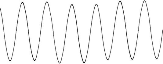
Before I start, I want to clarify the terms used to define a wave, which I use in the next few sections, and the relations between these terms (see Figure 1.1). There are four variables that we use to define any sinusoidal wave:
● The amplitude, A: How high each peak of the wave is in relation to the middle, its zero value.
● The frequency, f: The number of ups and downs in the wave in a given time. The units are Hertz or number of ups and downs per second: a number/s.
● The wavelength, λ: The distance between two peaks, in meters (m), centimeters (cm), or micrometers (μm).
● The wave number, ν (the Greek letter nu, not the letter v): The reciprocal of the wavelength. Some properties of waves are better expressed by the reciprocal of the wavelength. The units are therefore 1/m or m−1, or cm−1, or μm−1.
Semiconductor Basics: A Qualitative, Non-mathematical Explanation of How Semiconductors Work and How They Are Used, First Edition. George Domingo. © 2020 John Wiley & Sons Ltd. Published 2020 by John Wiley & Sons Ltd.
The last three variables are related by the velocity of the wave. Velocity is the distance that a moving object covers during a fixed amount of time, so the velocity v (this is now the letter v) has units of meters per second (m/s). The key relationships are
and the wave number – the reciprocal of the wavelength – is
For example, suppose that Figure 1.1 represents a sound wave. The velocity of sound in air is 343 m s−1. Take a look at Figure 1.1:
● The figure shows 5 cycles in 0.001 seconds, which means the frequency is 5000 cycles per second or f = 5000 Hz, (where Hz, Hertz is the unit for frequency) which happens to be the middle of our hearing range.
● The wavelength is the velocity divided by the frequency, or λ = 343 (m s−1)/5000 (1 s−1) = 0.069 m or 6.9 cm. Notice that the seconds cancel out, and therefore the units are in meters or centimeters.
● The wave number is v = 1/0.069 m = 14.5 m−1.
As much as possible, I use the metric system of units (MKS, meter, kilogram, second). I have always found it very annoying when books keep changing the unit system. When necessary, I will give you the equivalents.
Frequency, f (number of cycles per second)
0.001s
Wavelength, λ (m)
Reciprocal of the wavelength, v (1/m)
Time
Amplitude
Figure 1.1 A sinusoidal wave is described in several ways: frequency, wavelength, and reciprocal of the wavelength plus its amplitude.
Now we are ready to dive into the pre-history of the Bohr atom and understand how Dr. Bohr came up with his famous model.
1.2 The Case of the Missing Lines
To explain how semiconductors work, we start with the Bohr atom. Most readers are familiar with Bohr’s planetary model of the atom. How Bohr came up with this model is a very interesting scientific historical path involving many famous scientists of the nineteenth and early twentieth centuries. Science goes one step at a time.
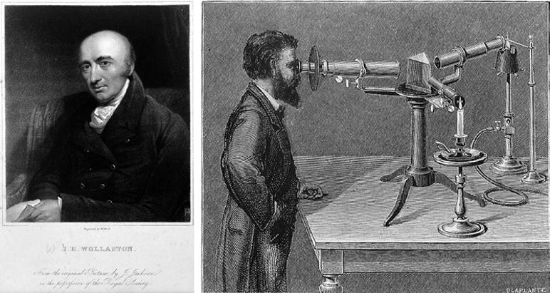
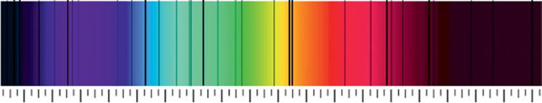
William Wollaston (1766–1826), shown on the left in Figure 1.2, was an English chemist who discovered a couple of atomic elements, including palladium and rhodium. Very early in the 1800s, he built the first spectrometer. Wollaston focused the light from the sun through a prism and, to his surprise, found black lines partitioning the spectra (Figure 1.3). What the heck was going on?
Figure 1.2 William Wollaston (left) looked at the sun’s light through a prism and was the first to observe the missing lines. Source: https://library.si.edu/image-gallery/73731. Joseph von Fraunhofer (right) studied the missing lines with his spectrometer and named them A–K. where Hz, Hertz is the unit for frequency. https://www.kruess.com/en/campus/spectroscopy/history-of-spectroscopy/
Figure 1.3 The sun’s spectrum through a prism shows dark lines: wavelengths of light that seem to have disappeared. Source: https://www.kruess.com/en/campus/spectroscopy/history-ofspectroscopy/. (Shehe Miaher o r C c l r rheprheahei C M i o TMa oMngurhe)
Suppose you are roasting a chicken and carefully watching the dial of a digital thermometer inserted in the chicken’s breast as the temperature increases from room temperature, 24 °C (degrees Celsius), to 80 °C, the recommended internal temperature of a well-cooked chicken breast. As the temperature increases, suddenly the thermometer jumps from 39 °C to 41 °C, then from 56 °C to 58 °C, and finally from 66 °C to 68 °C. You wonder what is wrong with the thermometer: why don’t the temperatures 40, 57, and 67 °C show up on the dial? They don’t seem to exist. You buy a new thermometer, just to be sure, and find that exactly the same temperature values are missing. A third thermometer gives the same results. You place the same thermometers in soup, and the thermometers are well behaved, showing in succession the values 39, 40, and 41 °C. So, the thermometers work. The missing temperatures are no coincidence. There is something in that chicken that makes the temperature jump from one value to another without passing through the one in the middle.
Well, that was probably Wollaston’s initial reaction. What separated the colors? Was the instrument lens dirty? He even considered the possibility that there were natural boundaries between certain colors. But why didn’t these black boundaries appear when he pointed the spectrometer at a white light?
German physicist Joseph von Fraunhofer (1787–1826), on the right in Figure 1.2, studied these dark lines of the sun’s spectrum in much more detail and actually named the missing lines with the letters A–K (not too imaginative; ancient astronomers would have found much more attention-grabbing names).
1.3 The Strange Behavior of Spectra from Gases and Metals
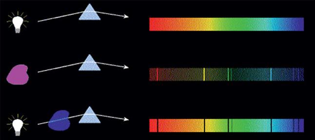
The next step was to take a look at the emission of light from several metals, gases, and stars. The observers soon found that each element has its own unique set of lines. Take a look at Figure 1.4. White light through a prism generates a continuous spectrum (top diagram); no colors are missing. If we heat a gas until it glows and pass the light through the same prism (middle diagram), only certain lines are projected onto the screen: the rest of the
Figure 1.4 The spectrum from any gas shows similar but different missing lines (middle image), but when the same gas is hot and emits light, only the lines that were black before are now visible (lower image). Source: https://quizlet.com/102018176/astronomy-4-spectroscopy-flash-cards/. (Shehe Miaher o r C c l r rheprheahei C M i o TMa oMngurhe)
1.5 The Hyr ngheiSphec ruum Mihea 5 spectrum has disappeared. But if we do it differently – that is, if we have the cold gas between the white light and the prism (bottom diagram) – then the full spectrum appears, except for exactly the same lines that were visible in the previous spectral measurement. The superposition of the middle and lower spectra is equal to the spectrum of the white light at the top. The gas, when cold, absorbs the same specific light waves as the ones it emits when it glows. What a coincidence! And this happens with all gases and materials. The lines are at different frequencies, but all of them have lines.
1.4 The Classifications of Basic Elements
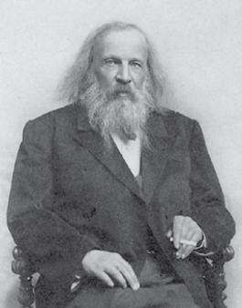
In 1766, an English aristocrat named Henry Cavendish (1731–1810) was the first to recognize hydrogen as an element, that is, a unique substance and an integral part of the water molecule. By the time Dmitri Mendeleev (1834–1907) published his now ubiquitous periodic table of the elements in 1869, 100 years later, it was already known that hydrogen was the lightest of all the known elements (at that time, 60 elements were known). Mendeleev (Figure 1.5) reordered the known elements by their relative atomic weight, with hydrogen as 1.
Figure 1.5 Dmitri Mendeleev and the periodic table with the elements known in his time and the empty slots for elements still to be discovered. Source: Wikipedia, https://en.wikipedia.org/wiki/ Dmitri_Mendeleev#/media/File:Dmitri_Mendeleev_1890s.jpg.
1.5 The Hydrogen Spectrum Lines
Johann Balmer (1825–1898), a Swiss mathematician, found empirically in 1895 that the separation of the optical lines generated by hydrogen gas can be expressed by a formula using just a constant, C, and integer numbers. He expressed his observation with Eq. (1.3)
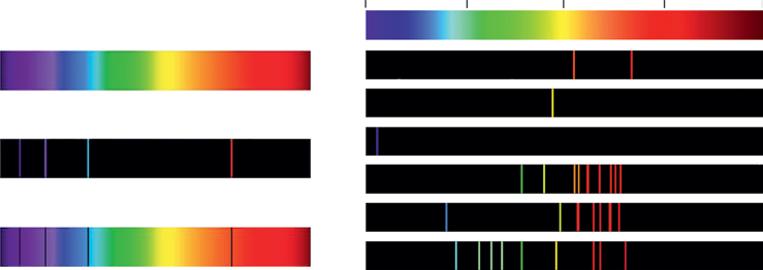
Figure 1.6 The spectrum of the hydrogen atom on the left shows the absorption lines (below) and the emission lines (middle). On the right are the emission lines of several other materials. Source: https://www.shutterstock.com/image-vector/spectrum-spectral-line-example-hydrogenemission-1288942888?src=iUiOwiDEznOcV6XzswXhMA-1-0 (left); https://www.shutterstock. com/image-vector/line-spectra-elements-339037577?src=I6tWF1qlh6XcWayXsZl-Gw-3-16 (right). ( Shehe Miaher o r C c l r rheprheahei C M i o TMa oMngurhe )
here λ is the wavelength of the missing line, C is a heuristically obtained constant (C = 3.64 × 10⁻⁹ m), n = 2, and m is an integer greater than 2 (i.e. 3, 4, 5, and so on). When you put any of these integer numbers in Eq. (1.3), you get the wavelength of all the lines in the hydrogen spectrum.
Figure 1.6 shows the hydrogen spectrum on the left, with its characteristic emission and absorption lines. These are the lines that Balmer used to develop Eq. (1.3) to calculate the missing hydrogen’s wavelengths. All the elements have similar absorption and emission lines at different wavelengths, and I show a few on the right in Figure 1.6.
Just three years later, Johannes Rydberg (1854–1919) found that the Balmer equation was one specific case of a more general formula, Eq. (1.4):
The reciprocal of the wavelength is now given by a constant R and the same integer numbers, except that now n is allowed to have different integer numbers: 2, 3, 4, and so on. R is also a heuristically derived constant (R = 1.1 × 10⁷ m−1), called the Rydberg constant. Both Balmer and Rydberg (Figure 1.7) were able to quantify the entire spectrum of the hydrogen atom using the relationship in Eq. (1.4). It is interesting that Niels Bohr, whom I’ll talk more about in Section 1.8, was able to calculate the Rydberg number using fundamental physical values, such as the mass of the electron, the electronic charge, the permittivity of free space, Planck’s constant, and the speed of light (see Appendix 1.3). This behavior screams for an explanation.

1.7 Johann Balmer (left) found a mathematical relation for hydrogen’s spectral lines, and Johannes Rydberg (right) came up with a more general equation applicable to all gases and materials. Source Wikipedia, https://en.wikipedia.org/wiki/Johann_Jakob_Balmer#/media/File:Balmer. jpeg (left); Wikipedia, https://en.wikipedia.org/wiki/Johannes_Rydberg#/media/File:Rydberg,_Janne_ (foto_Per_Bagge;_AFs_Arkiv).jpg (right).
1.6 Light is a Particle
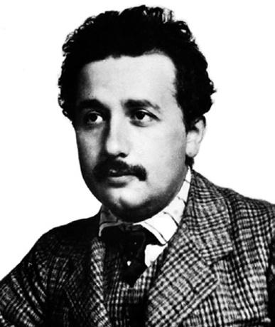
Albert Einstein (1879–1955, Figure 1.8) published a paper in 1905 on the theory of the photoelectric effect. When light strikes a metal surface, it frees an electron if its energy is higher than a given threshold value. Any remaining energy is used to kick the electron off the surface. In his paper, Einstein proposed the concept that light has a dual personality; it behaves like a wave or like a particle, and the particle has an energy associated with the wavelength of that light.
He called this particle a “light quantum.” (In 1926, a French physicist named Frithiof Wolfers [1891–1971] renamed the light quantum a photon. It is interesting that Einstein received the Nobel Prize in 1921 for the discovery of the photon, not for his much more famous work on relativity.) This light particle, the photon, has an energy that depends on the frequency of the light. The energy associated with this light is given by the formula Ehf hc (1.5)
where h is Planck’s constant (h = 6.63 10−34 m2 kg s−1), c is the speed of light (c = 3 × 10⁸ m s−1), and λ is the wavelength (m). The meter in the numerator cancels the one in the denominator, resulting in the energy given in Joules (= kg m2 s−2).
Figure
1.7 The Atom’s Structure
Figure 1.8 Around 1905, Albert Einstein came up with the concept that light behaves as both a wave and a particle. Source: Wikipedia, https://en.wikipedia.org/wiki/ Albert_Einstein#/media/File:Einstein_ patentoffice.jpg.
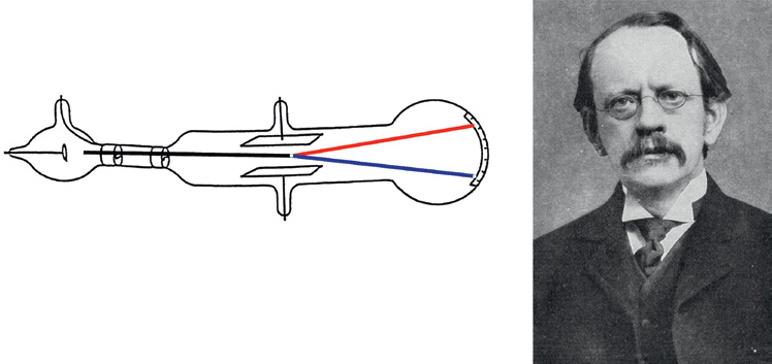
While all of these light experiments and relationships were being observed in the late nineteenth century, other scientists were playing with cathode-ray tubes, the precursors of old television sets and oscilloscopes, trying to understand the nature of the atom. The cathode-ray tube consists of an evacuated tube with two contacts, one at each end: the cathode and the anode. When a voltage is applied across the tube, current flows from the cathode to the anode, and the tube glows. The scientists explained this phenomenon by saying that electrons going through an evacuated tube containing very few atoms are able to attain sufficient velocity (and therefore kinetic energy) to hit the atoms and make them glow. They were called cathode rays.
Nobel Prize winning British physicist Joseph John Thomson (1856–1940, Figure 1.9) studied cathode rays and postulated in 1897 that they consisted of extremely small negatively charged particles, which he initially called “corpuscles.” (As happened with the term photon, George Stoney (1826–1911) later renamed corpuscles as electrons.) By studying how these particles moved through the gas and how they could be deflected by magnets, Thomson concluded that the “corpuscles” were (i) negatively charged particles and (ii) much smaller than the atoms themselves – at least 1000 times smaller. To account for electrically neutral atoms, he proposed that there is a core of positive charges with a large mass surrounded by an amorphous cloud of negatively charged electrons.
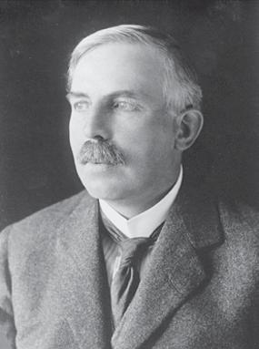
Ernest Rutherford (1871–1937, Figure 1.10), also a Nobel Prize winner, worked with radioactivity. In 1911, he bombarded very thin gold foil with alpha particles and looked at the scattered reflections as the radiation went through the foil. Most of the radiation went through the foil undeflected. Only a few alpha particles were reflected back and, from the angle of the reflected radiation, he concluded that the atom must have a very small,
Figure 1.9 Joseph John Thomson and his cathode ray tube. Source: Wikipedia, https://en.wikipedia. org/wiki/J._J._Thomson#/media/File:JJ_Thomson_Cathode_Ray_2.png (left); Wikipedia, https://en. wikipedia.org/wiki/J._J._Thomson#/media/File:J.J_Thomson.jpg (right).
Figure 1.10 Ernest Rutherford, with his experiment that bombarded alpha particles with radiation, concluded that the nucleus is extremely small and is concentrated at the center of the atom. Source: Wikipedia, https://upload.wikimedia.org/wikipedia/commons/6/6e/Ernest_Rutherford_LOC.jpg.
concentrated, positively charged core to compensate for the negatively charged electrons. Because the large majority of alpha particles passed through the foil without any directional change, he concluded that the majority of the space in an atom is empty, and the electrons are orbiting the nucleus instead of just being a scrambled negatively charged cloud as Thomson had suggested.
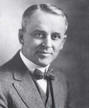
Robert Millikan (1868–1953, Figure 1.11) was able to measure the electrical charge of an electron with an interesting oil drop experiment in 1909. He suspended a very small charged
Figure 1.11 Robert Millikan, with his oil-drop experiment, measured the electrical charge of an electron. Source: https://en.wikipedia.org/wiki/Robert_Andrews_Millikan#/media/File:Millikan.jpg.
oil drop between two metal plates – one positive and the other negative – creating an electric field between the plates. He dropped tiny oil droplets into a vacuum chamber, and with X-rays, he negatively charged some of the oil drops. By changing the electric field between the two plates, he could control the speed of the oil drops, slowing them down, stopping them, or even moving them upward. By knowing the density of the oil drop, the size of the drop, its volume and mass, and the electric field that compensated for the effect of gravity, he was able to come up with the value of the charge of a single electron: 1.592 × 10⁻¹⁹ coulombs (he was off by less than 1% of the now-established number – not bad at all).
1.8 The Bohr Atom
So here we are in 1913 (just a mere 105 years ago at the time of this writing). What did Bohr know? He knew:
1) That a hydrogen atom is the simplest atom, consisting of just one proton (positively charged) and one electron (negatively charged).
2) That all of the atom’s mass is concentrated at the core: that is, the proton.
3) That electrons are negative particles somehow orbiting the nucleus.
4) That the great majority of space in an atom is empty.
5) That all the other elements can be organized neatly by weight on a periodic table.
6) That all elements have different emission spectra with specific emission or absorption color lines.
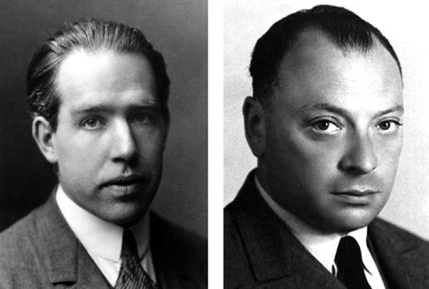
Niels Bohr (1885–1962, Figure 1.12) was able to beautifully explain all of these observations and how the spectral lines are generated. He postulated in 1912 that an atom consists of a core nucleus that has all the mass and is surrounded by electrons, moving like a planetary system in well-defined orbits (Figure 1.13). Electrostatic forces between the proton
Microscope
X-rays
1.12
postulated the planetary model of the atom. Wolfgang
using quantum mechanics, proved that no two electrons in a system can have the same quantum numbers. Source: Wikipedia, https://en.wikipedia.org/wiki/Niels_Bohr#/media/File:Niels_Bohr.jpg (left); Wikipedia, https://en.wikipedia.org/wiki/Wolfgang_Pauli#/media/File:Pauli.jpg (right).
Figure 1.13 The Bohr planetary model of an atom has discrete and stable orbits. An electron falling from level 3 to level 2 transfers its energy to an equivalently energetic photon.
n =3
n =2
n =1
f =∆E/h
and the electron (analogous to the gravitational forces in the solar system) keep the electrons circulating without escaping their orbit. Additionally, Bohr postulated that the electrons in orbit do not radiate any energy, so the orbits are stable. The only way to radiate or absorb any energy is for an electron to jump from one orbit to another, and that is precisely what explains the spectra of hydrogen and other elements.
Since electrons are forbidden to have any energy except for the energy of a specific orbit, they have to jump from one orbit to another, like going up the stairs, one, two, or three steps at a time (not one and a half). When falling from a higher orbit to a lower one, the electron releases a fixed packet of energy in the form of a photon of a very precise frequency (remember that Einstein said light behaves like a particle with an energy related to the wavelength of the light: Eq. 1.5). The transition from orbit 3 to orbit 2, as I show in
Figure
Niels Bohr (left)
Pauli (right),
Nucleus
Figure 1.13, results in the emission of a photon of a very precise frequency, given by the change in energy, ΔE, divided by Planck’s constant. Similarly, if an electron in orbit 2 wants to jump to orbit 3, the hydrogen atom has to absorb the energy it needs by absorbing a photon with the same precise energy, or by thermal heating, or by some other means. All other light photons not exactly matched to the difference between the energy levels go through the material unimpaired. The material is therefore transparent for all of the light waves that do not match the exact difference between two energy levels.
In 1924, Austrian Wolfgang Pauli (1900–1958, on the right in Figure 1.12) proposed his exclusion principle, which states that no two electrons (or fermion particles) in a system can have the same quantum numbers. The first atomic level of any element can hold only 2 electrons, the second 8, the third 18, the fourth 32, etc. A simple relation tells you how many electrons can share a given energy orbit: 2n2. You may wonder why. If, according to Pauli’s exclusion principle, the electrons cannot share the same quantum state, why do we have more than one electron in each orbit? The answer is that each electron is described by four quantum numbers (like the three numbers that describe your first, middle, last names, and your date of birth), but only the first quantum number, n, specifies the energy of the electron and thus explains the behavior of the light spectra. I explain the electron’s four quantum numbers in more detail in Appendix 1.1.
Here’s an analogy. Suppose I have a theater with 2 seats in the first row, 8 in the second, 18 in the third, 32 in the fourth, etc. The tickets for the first row cost $20, the second row $50, the third row $75, the fourth $125, and so on. (I know, it is a weird theater, but this is just an analogy.) Spectators are forbidden to sit in someone else’s lap or stand in the aisles. If 12 people show up for the performance, they first occupy the 2 seats of the first row, the next 8 patrons occupy the second row, and the last 2 spectators sit somewhere in the third row. Further back in the theater, the rows have more seats, but they are empty. If a patron wants to change rows – from row 3 to row 4, for example – he has to pay the extra $50: the difference in the price of the tickets in the different rows. If he moves the other way, from row 4 to row 3, he is reimbursed the $50. Now, if a wealthy person in row 1 wants to move to row 4, he will be required to pay $105. That is, money must be paid or received to move from one row to another. All these changes assume that the seat someone desires is unoccupied. If the group of spectators is short of money (no energy), they will occupy the seats of the first rows as long as there are seats available. If the group is wealthy (has lots of energy), they can jump from one seat to another as long as they have enough money (energy) to afford the higher prices. The amount they have to pay depends only on the difference in the price of the seats in each row. End of analogy.
At 0 K, absolute temperature (−273 °C), there is no energy whatsoever, so all the electrons occupy the lowest allowed energy levels. At room temperature, 300 °C, there is quite a large amount of thermal energy, and electrons start moving from one level to another, leaving empty seats that can be occupied by other electrons, absorbing or emitting photons as they move.
Figure 1.14 shows the transitions observed in the hydrogen atom. The groups of lines were named later by those who found them.
Have you ever wondered why, when we walk on the second floor, we do not fall through it and land on the first floor? Think about it. The typical size of an atom is 5 × 10⁻¹⁰ m, and the size of a nucleus is about 30 000 times smaller, 1.6 × 10⁻¹⁵ m. All the mass is