Repairable systems reliability analysis: a comprehensive framework john wiley & sons all chapter ins
Repairable Systems Reliability Analysis: A Comprehensive Framework
John Wiley & Sons
Visit to download the full and correct content document: https://ebookmass.com/product/repairable-systems-reliability-analysis-a-comprehensi ve-framework-john-wiley-sons/
More products digital (pdf, epub, mobi) instant download maybe you interests ...
Reliability Engineering, Third Edition (Wiley Series in Systems Engineering and Management) Elsayed A. Elsayed
For more information about Scrivener publications please visit www.scrivenerpublishing.com.
All rights reserved. No part of this publication may be reproduced, stored in a retrieval system, or transmitted, in any form or by any means, electronic, mechanical, photocopying, recording, or otherwise, except as permitted by law. Advice on how to obtain permission to reuse material from this title is available at http://www.wiley.com/go/permissions.
Wiley Global Headquarters
111 River Street, Hoboken, NJ 07030, USA
For details of our global editorial offices, customer services, and more information about Wiley products visit us at www.wiley.com.
Limit of Liability/Disclaimer of Warranty
While the publisher and authors have used their best efforts in preparing this work, they make no representations or warranties with respect to the accuracy or completeness of the contents of this work and specifically disclaim all warranties, including without limitation any implied warranties of merchantability or fitness for a particular purpose. No warranty may be created or extended by sales representatives, written sales materials, or promotional statements for this work. The fact that an organization, website, or product is referred to in this work as a citation and/or potential source of further information does not mean that the publisher and authors endorse the information or services the organization, website, or product may provide or recommendations it may make. This work is sold with the understanding that the publisher is not engaged in rendering professional services. The advice and strategies contained herein may not be suitable for your situation. You should consult with a specialist where appropriate. Neither the publisher nor authors shall be liable for any loss of profit or any other commercial damages, including but not limited to special, incidental, consequential, or other damages. Further, readers should be aware that websites listed in this work may have changed or disappeared between when this work was written and when it is read.
Library of Congress Cataloging-in-Publication Data
ISBN 978-1-119-52627-8
Cover image: Stockvault.Com
Cover design by Russell Richardson
Set in size of 11pt and Minion Pro by Manila Typesetting Company, Makati, Philippines
Printed in the USA 10 9 8 7 6 5 4 3 2 1
5.4
5.4.1
5.4.1.1
6
7
6.2.3
6.2.4
8
viii Contents
8.3
8.3.4
8.3.5
8.4
8.5
8.6
8.3.5.1
Series Editor Preface
This is the 10th book in the series on performability engineering since the series was launched in 2014. The subject of this book is special as not many books on Repairable System Reliability are available in the literature on reliability engineering. All the three authors of this book come from the reputed academic institutes of technology in India, but have also have had rich experience of working on field projects of practical importance. Incidentally, the two of the authors, namely, Rajiv Nandan Rai and Sanjay Kumar Chaturvedi are the postgraduate and doctorate, respectively, of the first Centre of Reliability Engineering established in India by the series Editor in 1983 at the Indian institute of Technology, at Kharagpur. Rajiv Nandan Rai has also served with the Indian Air Force and has had about 20 years of industrial experience in military aviation, which is reflected in the treatment of the subject.
Actually, the research in repairable systems reliability is limited and very few textbooks are available on the subject. The available textbooks generally provide coverage of non-homogeneous Poisson process (NHPP) where the repair effectiveness index (REI) is considered one. Few more textbooks provide treatment of non-parametric reliability analysis of repairable systems. However, this book aims to provide a comprehensive framework for the analysis of repairable systems considering both the non-parametric and parametric estimation of the failure data. The book also provides discussion of generalized renewal process (GRP) based arithmetic reduction of age (ARA) models along with its applications to repairable systems data from aviation industry.
Repair actions in military aviation may not fall under ‘as good as new (AGAN)’ and ‘as bad as old (ABAO)’ assumptions which often find limited uses in practical applications. But actual situation could lie somewhere between the two. A repairable system may end up in one of the five likely states subsequent to a repair: (i) as good as new, (ii) as bad as old, (iii) better than old but worse than new, (iv) better than new, and lastly, (v) worse than old. Existing probabilistic models used in repairable system analysis, such
x Series Editor Preface
as the perfect renewal process (PRP) and the non-homogeneous Poisson process (NHPP), account for the first two states. In the concept of imperfect repair, the repair actions are unable to bring the system to as good as new state, but can transit to a stage that is somewhere between new and that of one preceding to a failure. Because of the requirement to have more precise analyses and predictions, the GRP can be of great interest to reduce the modelling ambiguity resulting from the above repair assumptions. The authors have discussed to a great extent various possibilities under repairability environment and applied them to physical systems. The book also summarizes the models and approaches available in the literature on the analysis of repairable system reliability.
It is expected the book will be very useful to all those who are designing or maintaining repairable systems.
Krishna B. Misra Series Editor
Preface
Conventionally, a repair action usually is assumed to renew a system to its “as good as new” condition. This assumption is very unrealistic for probabilistic modeling and leads to major distortions in statistical analysis. Most of the reliability literature is directed toward non-repairable systems, that is, systems that fail are discarded. This book is mainly dedicated toward providing coverage to the reliability modeling and analysis of repairable systems that are repaired and not replaced when they fail.
During his journey in the military organization, the first author realized that most of the industries desire to equip its scientists, engineers, and managers with the knowledge of reliability concepts and applications but have not been able to succeed completely. Repairable systems reliability analysis is an area where the research work is quite limited and very few text books are available. The available text books are also limited in providing a coverage only up to the concepts of non-homogeneous Poisson process (NHPP) where the repair effectiveness index (REI) is considered one. Few more textbooks provide knowledge only on non-parametric reliability analysis on repairable systems.
This book provides a comprehensive framework for the modeling and analysis of repairable systems considering both the non-parametric and parametric estimation of the failure data. The book provides due exposure to the generalized renewal process (GRP)–based arithmetic reduction of age (ARA) models along with its applications to repairable systems data from aviation industry. The book also covers various multi-criteria decision making (MCDM) techniques, integrated with repairable systems reliability analysis models to provide a much better insight into imperfect repair and maintenance data analysis. A complete chapter on an integrated framework for procurement process is added which will of a great assistance to the readers in enhancing the potential of their respective organization. It is intended to be useful for senior undergraduate, graduate, and post-graduate students in engineering schools as also for professional engineers, reliability administrators, and managers.
xii Preface
This book has primarily emerged from the industrial experience and research work of the authors. A number of illustrations have been included to make the subject pellucid and vivid even to the readers who are new to this area. Besides, various examples have been provided to showcase the applicability of presented models and methodologies, besides, to assist the readers in applying the concepts presented in the book.
The concepts of random variable and commonly used discrete and continuous probability distributions can readily be seen in various available texts that deal with reliability analysis of non-reparable systems. The reliability literature is in plenty to cover such aspects in reliability data analysis where the failure times are modeled by appropriate life distributions. Hence, the readers are advised to refer to any such text book on nonrepairable systems reliability analysis for a better comprehension of this book.
Chapter 1 presents various terminologies pertaining to repairable systems followed by the description of repair concepts and repair categories.
The mean cumulative function (MCF)–based graphical and nonparametric methods for reparable systems are simple yet powerful option available to analyze the fleet/system events recurrence behavior and their recurrence rate. Chapter 2 is dedicated to MCF-based non-parametric analysis through examples with a case study of remotely operated vehicle (ROV).
The renewal and homogeneous Poisson processes (HPPs) followed by an exhaustive description of NHPP are covered in Chapter 3 along with solved examples. Thereafter, the chapter brings out a detailed description of ARA and ARI models along with their applicability in maintenance. The chapter also derives the maximum likelihood estimators (MLEs) for Kijima virtual age models with the help of GRP. The models are demonstrated with the help of suitable examples.
Chapter 4 provides various goodness-of-fit (GOF) tests for repairable systems and their applications with examples.
Chapter 5 presents various reliability and availability-based maintenance models for repairable systems. This chapter introduces the concept of high failure rate component (HFRC)–based thresholds and provides maintenance models by considering the “Black Box” (BB) approach followed by the failure mode (FM) approach. All the models are well-supported with examples.
This book presents modified failure modes and analysis (FMEA) model in Chapter 6. This model is based on the concept of REI propounded by Kijima and is best applicable to the repairable systems reliability analysis.
Chapter 7 provides an integrated approach for weapon procurement systems for military aviation. The combined applications of MCDM tools
Preface xiii
like AHP, ANP, and optimization techniques can be seen in this chapter. This model can be used for other industries procurement policy as well.
Chapter 8 is aimed at reducing the overhaul time of a repairable equipment to enhance the availability. Various concepts of throughput analysis have been utilized in this chapter.
The book makes an honest attempt to provide a comprehensive coverage to various models and methodologies that can be used for modeling and analysis of repairable systems reliability analysis. However, there is always a scope for improvement and we are looking forward to receiving critical reviews and/or comments of the book from students, teachers, and practitioners. We hope that the readers will all gain as much knowledge, understanding, and pleasure from reading this book as we have from writing it.
Rajiv Nandan Rai Sanjay Kumar Chaturvedi Nomesh Bolia August 2020
List of Tables
xvi List of Tables
Table
Table
Table
Table
Table
Table
Table 8.4 Process requirements of
Table 8.5
Table 8.6 Component 1—LPCR blades
Table 8.7 Component 2—CCOC
Table 8.8 Component 3—LPTR
List of Figures
Figure
Introduction to Repairable Systems
1.1 Introduction
A system is a collection of mutually related items, assembled to perform one or more intended functions. Any system majorly consists of (i) items as the operating parts, (ii) attributes as the properties of items, and (iii) the link between items and attributes as interrelationships. A system is not only expected to perform its specified function(s) under its operating conditions and constraints but also expected to meet specified requirements, referred as performance and attributes. The system exhibits certain behavioural pattern that can never ever be exhibited by any of its constituent items or their subsets. The items of a system may themselves be systems, and every system may be part of a larger system in a hierarchy. Each system has a purpose for which items, attributes, and relationships have been organized. Everything else that remains outside the boundaries of system is considered as environment from where a system receives input (in the form of material, energy, and/or information) and makes output to the environment which might be in different form as that of the input it had received. Internally, the items communicate through input and output wherein output(s) of one items(s) becomes the input(s) to others. The inherent ability of an item/system to perform required function(s) with specified performance and attributes when it is utilized as specified is known as functionability [1]. This definition differentiates between the terms functionality and functionability where former is purely related to the function performed whereas latter also takes into considerations the level of performance achieved.
Despite the system is functionable at the beginning of its operational life, we are fully aware that even after using the perfect design, best technology available for its production or the materials from which it is made, certain irreversible changes are bound to occur due to the actions of various interacting and superimposing processes, such as corrosion, deformations, distortions, overheating, fatigue, or similar. These interacting processes are the
main reason behind the change in the output characteristics of the system. The deviation of these characteristics from the specifications constitutes a failure. The failure of a system, therefore, can be defined as an event whose occurrence results in either loss of ability to perform required function(s) or loss of ability to satisfy the specified requirements (i.e., performance and/or attributes). Regardless of the reason of occurrence of this change, a failure causes system to transit from a state of functioning to a state of failure or state of unacceptable performance. For many systems, a transition to the unsatisfactory or failure state means retirement. Engineering systems of this type are known as non-maintained or non-reparable system because it is impossible to restore their functionability within reasonable time, means, and resources. For example, a missile is a non-repairable system once launched. Other examples of non-repairable systems include electric bulbs, batteries, transistors, etc. However, there are a large number of systems whose functionability can be restored by effecting certain specified tasks known as maintenance tasks. These tasks can be as complex as necessitating a complete overhaul or as simple as just cleaning, replacement, or adjustment. One can cite several examples of repairable systems one’s own day-to-day interactions with such systems that include but not limited to automobiles, computers, aircrafts, industrial machineries, etc. For instance, a laptop, not connected to an electrical power supply, may fail to start if its battery is dead. In this case, replacing the battery—a non-maintained item—with a new one may solve the problem. A television set is another example of a repairable system, which upon failure can be restored to satisfactory condition by simply replacing either the failed resistor or transistor or even a circuit board if that is the cause, or by adjusting the sweep or synchronization settings.
The system, in fact, wavers and stays between satisfactory and unsatisfactory states during its operational life until a decision is taken to dispense with it. The proportion of the time, during which the system is functionable, depends on the interaction between the inherent characteristics of a system from the design and utilization function given by the users’ specific requirements and actions. The prominent inherent characteristics could be reliability, maintainability, and supportability. Note that these characteristics are directly related to the frequency of failures, the complexity of a maintenance task, and ease to support that task. The utilization characteristics are driven by the users’ operational scenarios and maintenance policy adopted, which are further supported by the logistics functions, which is related to the provisioning of operational and maintenance resources needed. In short, the pattern followed by an engineering system can be termed as funtionability profile whose specific shape is governed by the inherent characteristics of design and system’s utilization. The metric
Availability or its variants quantitatively summarize the functionability profile of an item/system. It is an extremely important and useful measure for reparable systems; besides, a technical aid in the cases where user is to make decisions regarding the acquisition of one item among several competing possibilities with differing values of reliability, maintainability, and supportability. Functionability and availability brought together indicates how good a system is. It is referred as system technical effectiveness representing the inherent capability of the system. Clearly, the biggest opportunity to make an impact on systems’ characteristics is at the design stage to won or lost the battle when changes and modifications are possible almost at negligible efforts. Therefore, the biggest challenge for engineers, scientists, and researchers has been to assess the impact of the design on the maintenance process at the earliest stage of the design through field experiences, analysis, planning and management. And, the repairable system analysis is not just constricted on finding out the reliability metrics.
Most complex systems, such as automobiles, communication systems, aircraft, engine controllers, printers, medical diagnostics systems, helicopters, train locomotives, and so on so forth are repaired once they fail. In fact, when a system enters into utilization process, it is exposed to three different performance influencing factors, viz., operation, maintenance, and logistics, which should be strategically managed in accordance with the business plans of the owners. It is often of considerable interest to determine the reliability and other performance characteristics under these conditions. Areas of interest may include assessing the expected number of failures during the warranty period, maintaining a minimum reliability for an interval, addressing the rate of wear out, determining when to replace or overhaul a system, and minimizing its life cycle costs.
Traditional reliability life or accelerated test data analysis—nonparametric or parametric—is based on a truly random sample drawn from a single population and independent and identically distributed (i.i.d.) assumptions on the reliability data obtained from the testing/fielded units. This i.i.d. assumption may also be valid, intuitively, on the first failure of several identical units, coming from the same design and manufacturing process, fielded in a specified or assumed to be in an identical environment. Life data of such items usually consists of an item’s single failure (or very first failure for reparable items) times with some items may be still surviving-referred as censoring or suspension. The reliability literature is in plenty to cover such aspects in reliability data analysis where the failure times are modeled by appropriate life distributions [2].
However, in repairable system, one generally has times of successive failures of a single system, often violating the i.i.d assumption. Hence, it is
not surprising that statistical methods required for repairable system differ from those needed in reliability analysis of non-repairable items. In order to address the reliability characteristics of complex repairable systems, a process rather than a distribution is often used. For a repairable system, time to next failure depends on both the life distribution (the probability distribution of the time to first failure) and the impact of maintenance actions performed after the first occurrence of a failure. The most popular process model is the Power Law Process (PLP). This model is popular for several reasons. For instance, it has a very practical foundation in terms of minimal repair—a situation when the repair of a failed system is just enough to get the system operational again by repair or replacement of its constituent item(s). Second, if the time to first failure follows the Weibull distribution, then the Power Law model repair governs each succeeding failure and adequately models the minimal repair phenomenon. In other words, the Weibull distribution addresses the very first failure and the PLP addresses each succeeding failure for a repairable system. From this viewpoint, the PLP can be regarded as an extension of the Weibull distribution and a generalization of Poisson process. Besides, the PLP is generally computationally easy in providing useful and practical solutions, which have been usually comprehended and accepted by the management for many real-world applications.
The usual notion and assumption of overhauling of a system is to bringing it back to “as-good-as-new” (AGAN) condition. This notion may not be true in practice and an overhaul may not achieve the system reliability back to where it was when the system was new. However, there is concurrence among all the stakeholders that an overhaul indeed makes the system more reliable than just before its overhaul. For systems that are not overhauled, there is only one cycle and we are interested in the reliability characteristics of such systems as the system ages during its operational life. For systems that are overhauled several times during their lifetime, our interest would be in the reliability characteristics of the system as it ages during its cycles, i.e., the age of the system starts from the beginning of the cycle and each cycle starts with a new zero time.
1.2 Perfect, Minimal, and Imperfect Repairs
As discussed earlier, a repairable system is a system that is restored to its functionable state after the loss of functionability by the actions other than replacement of the entire system. The quantum of repair depends upon various factors like criticality of the component failed, operational status of the system, risk index, etc. Accordingly, the management takes a decision on
how much repair a system has to undergo. The two extremes of the repair are perfect and minimal repairs. A system is said to be perfectly repaired, if the system is restored to AGAN condition (as it is replaced with a new one). Normally, a perfect repair in terms of the replacement is carried out for very critical components, which may compromise operation ability, safety of the system, and/or personnel working with the system. On the other hand, a system is said to be minimally repaired, if its working state is restored to “as-bad-as-old” (ABAO). This type of repair is undertaken when there is heavy demand for the system to work for a finite time or the system will be undergoing preventive maintenance shortly or will be scrapped soon.
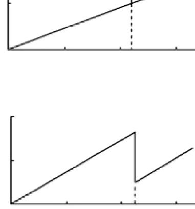
Any repair other than perfect and minimal repair comes under imperfect repair. Most of the repairs observed in day-to-day systems are imperfect repairs, i.e., a system is neither restored to AGAN conditions nor to ABAO conditions. The three types of repairs are pictorially represented in Figure 1.1.
Figure 1.1 Types of repair.
Repairable Systems Reliability Analysis
It can be seen from Figure 1.1 that in case of perfect repair, the system is rendered “AGAN” and the life starts at zero in the time scale signifying that the performance degradation is completely restored. In case of minimal repair, after the system is subjected to a repair action, its age remains same as before the repair action and there is no restoration of life below the previous age. So far the general repair is concerned, some of its life is renewed and the system starts functioning after being restored to somewhere between “ABAO” and “AGAN” state.
Figure 1.2 summarizes the techniques in vogue for reliability analysis for both repairable and non-repairable items, respectively.
Live Data Analysis (For Non-Repairable Items)
Parametric Analysis
Analysis Recurrent Event Data Analysis (For repairable Items) Failure Data Analysis
Analysis
Perfect Renewal Process (PRP)
General Renewal Process (GRP)
Distribution Weibull Distribution
Figure 1.2 Various techniques for reliability analysis.
Non-Homogenous Poisson Process (NHPP)
A renewal process (RP) is a counting process where the inter-occurrence times are stochastically i.i.d. with an arbitrary life distribution. Under the RP, a single distribution can characterize the time between failures (TBF), and the frequency of repair appears constant. The non-renewal behavior occurs if this frequency of repairs increases (deteriorating systems) or decreases (system improving) influencing the corresponding maintenance costs. The homogeneous Poisson process (HPP) describes a sequence of statistically i.i.d. exponential random variables. Conversely, a nonhomogeneous Poisson process (NHPP) [3, 4] describes a sequence of random variables that are neither statistically independent nor identically distributed. The NHPP is often used to model repairable systems that are subject to minimal repair. The generalized renewal process (GRP) allows the goodness of repairs within two extremities, viz., AGAN repair (RP) to the same-as-old repair (NHPP). The GRP is particularly useful in modeling the failure behavior of a specific unit and understanding the effects of repair actions on the age of that system. An example of a system to which the GRP is especially applicable is a system, which is repaired after a failure and whose repair neither brings the system to an AGAN or an ABAO condition, but instead partially rejuvenates the system. Therefore, one should be cautious on the fact that without looking at the actual behavior of the data may lead to underestimation or overestimation of engineering metrics.
The analysis by employing the parametric methods on scenarios of failure-repair requires a certain degree of statistical knowledge, the ability to solve complex equations and verification of distributional assumptions. Further, these equations cannot be solved analytically and require an iterative procedure or special software. Besides, parametric approaches are computationally intensive and not intuitive to a novice or an average person. The analysis of events, irrespective of the nature of the systemreparable or not reparable, should take an analysis path from nonparametric to versatile parametric model with graphical analysis being a common denominator. Undoubtedly, the choice of method depends on the data available and the questions we wish to answer.
1.3 Summary
A repairable system is a system that is restored to its functionable state after the loss of functionability by the actions other than replacement of the entire system. The two extremes of the repair are perfect and minimal repairs. A system is said to be perfectly repaired, if the system is restored
to AGAN condition (as it is replaced with a new one). On the other hand, a system is said to be minimally repaired, if its working state is restored to ABAO. Any repair other than perfect and minimal repair comes under imperfect repair. Most of the repairs observed in day-to-day systems are imperfect repairs, i.e., a system is neither restored to AGAN conditions nor to ABAO conditions. The RP is used to model AGAN condition. The NHPP is often used to model repairable systems that are subject to minimal repair. The GRP allows the goodness of repairs within two extremities, viz., AGAN repair (RP) to the same-as-old repair (NHPP).
The next chapter describes the mean cumulative function (MCF) based graphical and non-parametric methods for repairable systems.
References
1. Knezevic, J., Systems Maintainability, Analysis, Engineering and Management, Chapman and Hall, London, 1997.
2. Ebeling, C.E., An Introduction to Reliability and Maintainability Engineering, McGraw Hill, New York, 2007.
3. Rigdon, S.E. and Basu, A.P., Statistical Methods for the Reliability of Repairable Systems, Wiley, New York, 2000.
4. Ascher, H. and Feingold, H., Repairable Systems Reliability, Marcel Dekker, New York, 1984.
2
Repairable Systems Reliability Analysis: Non-Parametric
2.1 Introduction
Many products experience repeated repairs that requires special statistical treatment with respect to formulating methods and models for analysis. The items are usually considered statistically independent, but the times between the occurrences of failure or repair events within a system unit are neither necessarily independent nor identically distributed. The data are usually censored in the sense that system units have different ends of operational histories. A distributional analysis might also be possible for the systems’ which undergo a series of failure/repair cycles, on their very first observed failure or if their times-between-failures (TBF) show no trends. However, if a series of multiple failure or repair events, occurring sequentially in time continuum, are to be considered for analysis then order of the failure event’s occurrence does matter and ignorance would lead to incorrect analysis and decisions thereof [1, 2]. Since the collection of random variables involved in such systems evolve with time, their behavior is generally modeled through a process rather than a distribution. In reliability engineering, the systems under this category are commonly referred as repairable systems, i.e., systems that are brought to their normal functionable states by means of any minor or major maintenance action(s). Therefore, when assessing and analyzing the system reliability, it is always important to make the distinction between non-repairable components and repairable systems to select an appropriate approach.
For a company or for a competing manufacturer, the common concerns can be [3, 4]:
• The number of repairs, on average, for all system at a specified operational time?
• Expected time to first repair, subsequent repairs, etc.
• Trends in repair rate or costs whether increasing, decreasing, or substantially constant.
• How to take decisions on burn-in requirements and maintenance or retirement.
• Is burn-in would be beneficial? How long and costs effective it would be?
• How to compare different versions, designs, or performance of systems operating in different environment/ regions, etc.
Each of the above questions and many more can be answered by the method presented in this chapter. This chapter describes mean cumulative function (MCF) based non-parametric graphical approach—a simple yet powerful and informative model—to deal with failure events of systems undergoing a failure and repair cycles wherein the time to effect a repair is assumed to be negligible. This is a reasonable assumption with respect to the operational times of a unit that are usually long than its repair times.
The MCF approach is simple as it is easy to understand, prepare, and present the data. The MCF model is non-parametric in the sense that its estimation involves no assumptions about the form of the mean function or the process generating the system histories. Further, this graphical method allows the monitoring of system recurrences and the maintenance of statistical rigidity without resorting to complex stochastic techniques.
Further, the non-parametric MCF analysis provides similar information as probability plots in a traditional life data analysis. Especially, the plot of the nonparametric estimate of the population MCF yields most of the information sought and the plot is as informative as is the probability plot for life and other univariate data. The sample MCF can be estimated and plot can be constructed for just one single machine or for an entire fleet of machines in a population. Besides, it can also be constructed for all failures events, outages, system failures due to specific failure modes, etc. It can be used to track field recurrences and identify recurrence trends, anomalous systems, unusual behavior, the effect of various parameters (e.g., maintenance policies, environmental, and operating conditions, etc.) on failures, etc. For some situations, this is the only analysis we need to do, and in others, it becomes a precursor to a more advance parametric form of analysis.
2.2 Mean Cumulative Function
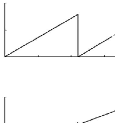
A common and popular reliability metric of a repairable system is the cumulative number of failure or repair events, N(t), occurring by time t (also termed as system age). Here, age (or time) means any measure of item’s usage, e.g., millage, kilometers, cycles, months, days, and so on. An item’s latest observed age is called its suspension or censored age beyond which its history is yet to be observed. A sample item may also not have observed a single failure whereas others have observed one, two, or more failures before its suspension age. Obviously, the number of events occurring by time is random. In non-parametric failure (or repair) events data analysis, every unit of the population can be described by a cumulative history function for the number of failures. The population average of cumulative number of failures (or repairs) at through time t is called Mean Cumulative Function (MCF), M(t)(= E(N(t))). Its derivative, mt dM t dt () () = , is assumed to exist and is termed as recurrence rate or intensity function or population instantaneous repair rate at time t. This rate may remain constant, increasing or decreasing in its characteristics and is expressed in terms of occurrences per unit population item per unit time. It is a staircase function with a jump at each event occurrence in time and tracking the accumulated number of events by time t of interest. It is the mean of all staircase functions of every unit in the population.
Figure 2.1 shows an example of the cumulative history function for a single system. The graph on cumulative number of failure events versus
Figure 2.1 A MCF example.
12 Repairable Systems Reliability
Analysis
the system age, t. This graph can be viewed as a single observation from a possible curve.
Let us take an example to illustrate the behavior of three units of identically designed systems operating under different environments or maintenance scenarios through MCF.
Example 2.1
Consider of three reparable systems observed until the time of their 12th failure the failure data [5].
System 1: 3, 9, 20, 25, 41, 50, 69, 91, 128, 151, 182, and 227.
System 2: 9, 20, 65, 88, 104, 107, 138, 143, 149, 186, 208, and 227.
System 3: 45, 76, 113, 129, 152, 174, 193, 199, 210, 219, 224, and 227.
Figures 2.2, 2.3, and 2.4, respectively, show the graphs of N(ti) versus ti
It is evident from the plots in Figures 2.2 to 2.4 that the three identical systems are behaving differently wherein the repair rates of these systems show decreasing (an improving system), linear (a stable system), and increasing (a deteriorating system) trends, respectively. In the above, the actual number of events by time t provides an unbiased estimate of the population mean number of failures (or repairs) per system, M(t). This is valid in a situation where only a single system is available at the time of analysis and other systems would appear in future when this single system’s design is acceptable and satisfied the intended requirements. However, in many cases, we are concerned with an overall behavior and performance of several systems manufactured through identical processes