Electrical Systems 2
From Diagnosis to Prognosis
Edited by
Abdenour Soualhi Hubert Razik
First published 2020 in Great Britain and the United States by ISTE Ltd and John Wiley & Sons, Inc.
Apart from any fair dealing for the purposes of research or private study, or criticism or review, as permitted under the Copyright, Designs and Patents Act 1988, this publication may only be reproduced, stored or transmitted, in any form or by any means, with the prior permission in writing of the publishers, or in the case of reprographic reproduction in accordance with the terms and licenses issued by the CLA. Enquiries concerning reproduction outside these terms should be sent to the publishers at the undermentioned address:
ISTE Ltd
John Wiley & Sons, Inc.
27-37 St George’s Road 111 River Street London SW19 4EU Hoboken, NJ 07030
UK USA
www.iste.co.uk
www.wiley.com
© ISTE Ltd 2020
The rights of Abdenour Soualhi and Hubert Razik to be identified as the authors of this work have been asserted by them in accordance with the Copyright, Designs and Patents Act 1988.
Library of Congress Control Number: 2019956924
British Library Cataloguing-in-Publication Data
A CIP record for this book is available from the British Library
ISBN 978-1-78630-608-1
Chapter 2. Signal Processing Techniques for Transient Fault
José Alfonso Antonino DAVIU and Roque Alfredo Osornio RIOS
2.1.
2.2.
2.2.1.
2.2.2.
2.3. Signal processing tools for transient
2.3.1. Example of a discrete tool: the DWT
2.3.2.
2.4. Application of transient-based tools for electric motor
2.4.1. Application of the DWT for the detection of rotor
2.4.2. Application of the HHT for the detection of
2.5.
2.6.
Chapter 3. Accurate Stator Fault Detection
3.1.
3.2.
3.2.2.
3.3. Extracting stator
3.4.
3.4.1.
3.4.2.
3.4.3.
3.5.
3.6.
Chapter 4. Bearing Fault Diagnosis in Rotating Machines
Claude DELPHA, Demba DIALLO, Jinane HARMOUCHE, Mohamed BENBOUZID, Yassine AMIRAT and Elhoussin ELBOUCHIKHI
4.1. Introduction
4.1.1. Bearing
4.1.2.
4.2. Method description
4.2.1.
4.2.2.
4.3. Experimental
4.3.1.
4.3.2. Time-domain
4.4. Global spectra
4.4.1.
4.4.2.
4.4.3.
4.5.
4.6.
Zhongliang LI, Zhixue ZHENG and Fei GAO
5.1.
5.2. PEMFC
5.2.1.
5.2.2.
5.3. Faults and degradation of PEMFCs
5.3.1.
5.3.2.
5.3.3. Variables used for PEMFC
5.4. PEMFC
5.4.1.
5.4.2.
5.4.3.
5.5. Prognosis of PEMFCs
5.5.1. Health index and EoL
5.5.2. Model-based prognostic
5.5.3. Data-driven and hybrid
5.5.4.
5.6. Remaining
5.7.
Introduction
The diagnosis and prognosis of electrical systems is still a relevant field of research. The research that has been carried out over the years has made it possible to acquire enough knowledge, to build a base from which we can delve further into this field of research. This study is a new challenge that estimates the remaining lifetime of the analyzed process. Many studies have been carried out to establish a diagnosis of the state of health of an electric motor, for example. However, making a diagnosis is like giving binary information: the condition is either healthy or defective. Of course, this may seem simplistic, but detecting a failure requires the use of suitable sensors that provide signals. These will be processed to monitor health indicators (features) for defects. Then, we witnessed a multitude of research activities around classification. It was indeed appropriate to distinguish the operating states, to differentiate them from one another and to inform the operator of the level of severity of a failure or even of the type of failure among a predefined panel. A major effort has been made to estimate the remaining lifetime or even the lifetime consumed. This is a challenge that many researchers are still trying to meet.
This book, which has been divided into two volumes, informs readers about the theoretical approaches and results obtained in different laboratories in France and also in other countries such as Spain, and so on. To this end, many researchers from the scientific community have contributed to this book by sharing their research results.
Introduction written by Abdenour SOUALHI and Hubert RAZIK
Chapter 1, Volume 1, “Diagnostic Methods for the Health Monitoring of Gearboxes”, by A. Soualhi and H. Razik, presents state-of-the-art diagnostic methods used to analyze the defects present in gearboxes. First of all, there is a bibliographical presentation regarding different types of gears and their defects. We conclude that gear defects represent the predominant defect at this level, thus justifying the interest in detecting and diagnosing them. Then, we present various gear analyses and monitoring techniques proposed as part of the condition-based maintenance and propose a diagnostic method. Thus, we show the three main phases of diagnosis: First, the analysis presented as a set of technical processes ensuring control of the representative quantities of operation; then the monitoring that exploits the fault indicators for detection; finally, the diagnosis which is the identification of the detected defect.
Chapter 2, Volume 1, “Techniques for Predicting Defects in Bearings and Gears”, by A. Soualhi and H. Razik, deals with strategies based on features characterizing the health status of the system to predict the appearance of possible failures. The prognosis of faults in a system means the prediction of the failure imminence and/or the estimation of its remaining life. It is in this context that we propose, in this chapter, the three methods of prognosis. In the first method, the degradation process of each system is modeled by a hidden Markov model (HMM). In a measured sequence of observations, the solution consists of identifying among the HMMs the one that best represents this sequence which allows predicting the imminence of the next degradation state and thus the defect of the studied system. In the second method (evolutionary Markov model), the computation of the probability that a sequence of observations arrives at a degradation state at the moment t+1, given the HMM modeled from the same sequence of observations, also allows us to predict the imminence of a defect. The third method predicts the imminence of a fault not by modeling the degradation process of the system, but by modeling each degradation state.
Chapter 3, Volume 1, “Electrical Signatures Analysis for Condition
Monitoring
of Gears
in
Complex Electromechanical Systems,”
written by S. Hedayati Kia and M. Hoseintabar Marzebali, deals with a review of their most remarkable research, which has been carried out in the last 10 years. A particular emphasis has been placed on the topic of noninvasive fault detection in gears using electrical signatures analysis. The main aim is to utilize the electrical machine as a sensor for the identification of gear defects. In this regard, a universal approach is developed for the first time by the authors which allows evaluating the efficacy of noninvasive techniques in the diagnosis of torsional vibration induced by the faulty gear located
within the drive train. This technique can be considered an upstream phase for studying the feasibility of gear fault detection using noninvasive measurement in any complex electromechanical system.
Chapter 4, Volume 1, “Modal Decomposition for Bearing Fault Detection”, by Y. Amirat, Z. Elbouchikri, C. Delpha, M. Benbouzid and D. Diallo, deals with induction machine bearing faults detection based on modal decomposition approaches combined to a statistical tool. In particular, a comparative study of a notch filter based on modal decomposition, through an ensemble empirical mode decomposition and a variational mode decomposition, is proposed. The validation of these two approaches is based on simulations and experiments. The achieved simulation and experimental results clearly show that, in terms of fault detection criterion, the variational mode decomposition outperforms the ensemble empirical mode decomposition.
Chapter 5, Volume 1, “Methods for Lifespan Modeling in Electrical Engineering”, by A. Picot, M. Chabert and P. Maussion, deals with the statistical methods for electrical device lifespan modeling from small-sized training sets. Reliability has become an important issue in electrical engineering because the most critical industries, such as urban transports, energy, aeronautics or space, are moving toward more electrical-based systems to replace mechanical- and pneumatic-based ones. In this framework, increasing constraints such as voltage and operating frequencies enhance the risk of degradation, particularly due to partial discharges (PDs) in the electrical machine insulation systems. This chapter focuses on different methods to model the lifespan of electrical devices under accelerated stresses. First, parametric methods such as design of experiments (DoE) and surface responses (SR) are suggested. Although these methods require different experiments to organize in a certain way, they reduce the experimental cost. In the case of nonorganized experiments, multilinear regression can help estimate the lifespan. In the second part, the nonparametric regression tree method is presented and discussed, resulting in the proposal of a new hybrid methodology that takes advantages of both parametric and nonparametric modeling. For illustration purpose, these different methods are evaluated on experimental data from insulation materials and organic light-emitting diodes.
Chapter 1, Volume 2, “Diagnosis of Electrical Machines by External Field Measurement”, by R. Pusca, E. Lefevre, D. Mercier, R. Romary and M. Irhoumah, presents a diagnostic method that exploits the information
delivered by external flux sensors placed in the vicinity of rotating electrical machines in order to detect a stator inter-turn short circuit. The external magnetic field measured by the flux sensors originates from the airgap flux density and from the end winding currents, attenuated by the magnetic parts of the machine. In the faulty case, an internal magnetic dissymmetry occurs, which can be found again in the external magnetic field. Sensitive harmonics are extracted from the signals delivered by a pair of flux sensors placed at 180° from each other around the machine, and the data obtained for several sensor positions are analyzed by fusion techniques using the belief function theory. The diagnosis method is applied on induction and synchronous machines with artificial stator faults. It is shown that the probability of detecting the fault using the proposed fusion technique on various series of measurements is high.
Chapter 2, Volume 2, “Signal Processing Techniques for Transient Fault Diagnosis”, by J.A. Daviu and R.A.O. Rios, revises the most relevant signal processing tools employed for condition monitoring of electric motors. First, the importance of the predictive maintenance area of the electric motors due to the extensive use of these machines in many industrial applications is pointed out. In this context, the most important predictive maintenance techniques are revised, showing the advantages such as the simplicity, remote monitoring capability and broad fault coverage of motor current analysis methods. In this regard, two basic approaches based on current analysis are explained: the classical methods, relying on the Fourier transform of steady-state current (motor current signature analysis – MCSA), and novel methods based on the analysis of startup currents (advanced transient current signature analysis – ATCSA). In the chapter, the most significant signal processing tools employed for MCSA and ATCSA are explained and revised. For MCSA, the basic problems derived from the application of the Fourier transform as well as other constraints of the methodology are explained. For ATCSA, the most suitable signal processing techniques are described, classifying them into continuous and discrete transforms. One representative of each group is accurately described (the discrete wavelet transform for discrete tools and the Hilbert-Huang transform for continuous tools), accompanying the explanation with illustrative examples. Finally, we discussed several examples of the application of each tool to electric motor fault diagnosis.
Chapter 3, Volume 2, “Accurate Stator Fault Detection in an Induction Motor Using the Symmetrical Current Components”, by M. Bouzid and G. Champenois, deals with the accurate detection of stator faults such as inter-turns short circuit, phase-to-phase and phase-to-ground faults of the
induction motor, using the symmetrical current components. The detection method is based on the monitoring of the behavior of the negative and zero sequence stator currents of the machine. This chapter also develops analytical expressions of these components obtained using the coupled inductance model of the machine. However, despite its efficiency, the negative sequence current-based method has its own limitations to detect accurate incipient stator faults in an induction motor. This limit can be explained by the fact that the negative sequence current generated in a faulty motor does represent not only the asymmetry introduced by the fault, but also by other superposed asymmetries, such as the voltage imbalance, the inherent asymmetry in the machine and the inaccuracy of the sensors. This aspect can generate false alarm and make the achievement of accurate incipient stator fault detection very difficult. Thus, to increase the accuracy of the fault detection and the sensitivity of the negative sequence current under different disturbances, this chapter proposes an efficient method able to compensate the effect of the different considered disturbances using experimental techniques having the originality to isolate the negative sequence current of each disturbance. The efficiency of all these proposed methods is validated experimentally on a 1.1-kW motor under different stator faults. Moreover, an original monitoring system, based on neural networks, is also presented and described to automatically detect and diagnose incipient stator faults.
Chapter 4, Volume 2, “Bearing Fault Diagnosis in Rotating Machines”, by C. Delpha, D. Diallo, J. Harmouche, M. Benbouzid, Y. Amirat and E. Elbouchikhi, is focused on detection, estimation and diagnosis of mechanical faults in electrical machines. Nowadays, it is necessary to rapidly assess the structural health of a system without disassembling its elements. For this in situ diagnosis purpose, the use of experimental data is very imperative. Moreover, the monitoring and maintenance costs must be reduced while ensuring satisfactory security performances. In this chapter, we focus on vibration-based signals combined with statistical techniques for bearing fault evaluation. Based on a four-step diagnosis process (modeling, preprocessing, feature extraction and feature analysis), the combination of several techniques such as principal components analysis and linear discriminant analysis in a global approach is explored to monitor the condition of vibration-based bearings. The main advantage of this approach is that prior knowledge on the bearing characteristics is not required. A particularly reduced frequency analysis has led to efficiently differentiate the bearing fault types and evaluate the bearing fault severities.
Chapter 5, Volume 2, “Diagnosis and Prognosis of Proton Exchange Membrane Fuel Cells”, by Z. Li, Z. Zheng and F. Gao, deals with the diagnostic and prognostic issues of fuel cell systems, especially the proton exchange membrane (PEMFC) type. First, the basic functioning principle of PEMFCs and their current development and application status are presented. Their high cost, low reliability and durability make them unfit for commercialization. In the following sections, degradation mechanisms related to both the aging effect and the system operations are analyzed. In addition, typical variables and characterization tools, such as polarization curve, electrochemical impedance spectroscopy, linear sweep voltammetry and cyclic voltammetry, are introduced for the evaluation of PEMFC degradation. Various diagnostic and prognostic methods in the literature are further classified based on their input-to-output process model of the system, namely model-based, data-driven and hybrid methods. Finally, two case studies for diagnosis and prognosis are given at the end of each part to give the readers a general and clearer illustration of these two issues.
Diagnosis of Electrical Machines by External Field Measurement
1.1. Introduction
Rotating electrical machines are found in all areas of modern domestic and industrial life [TAV 08]. They are the main electromechanical energy conversion devices in all industrial processes and have been widely used in different industrial applications for several decades. They account for approximately 70% of all electricity consumed on the grid and 80% of industrial engines involved in manufacturing processes. Regardless of the size of these units, from 1 kilowatt to several megawatts, the production losses due to a shutdown relating to an engine failure are greater than those induced by the actual engine efficiency. The failure of the machines, therefore, reduces the production rate and increases production and maintenance costs. It is then important to reduce maintenance costs and avoid unplanned downtime for these machines. Electrical machines must be monitored during the production process to improve their reliability and reduce their downtime [STO 04, ESE 17, NOR 93]. Monitoring of rotating electrical machines is still an essential part to increase reliability and operational safety of electrical systems and has been the subject of much research in recent decades [STO 04, HAN 10, PET 17].
Electric motors encounter a wide range of mechanical problems common to most machines, such as imbalance, misalignment, bearing faults and resonance [FOU 15, HAM 15, KAT 16]. But electric motors also encounter
Chapter written by Remus PUSCA, Eric LEFEVRE, David MERCIER, Raphael ROMARY and Miftah IRHOUMAH
their specific problems, which are the result of electromagnetic phenomena. The methods conventionally used for the diagnosis of electrical machines are based on measurements of current, voltage, vibration and noise. Although their effectiveness has been demonstrated, the generalization of these methods in the industrial environment remains limited on account of their relatively important cost.
Other methods based on magnetic field measurements outside the machine are interesting because they are inexpensive and easy to implement. Thus, monitoring devices based on the information provided by the magnetic flux produced by the imbalances in the magnetic or electrical circuit of the motors can be effectively used in addition to, or as an alternative to the current monitoring more conventionally used. Thus, many recent methods, used for the diagnosis of electrical machines, are based on the analysis of combining measurements of current and magnetic flux, where, on the basis of an evaluation of many tests, the stator current and the external leakage flux were selected as the most practical signals containing the information needed to detect broken bars and short circuit between turns of the stator winding [CEB 12a, YAZ 10].
The methods presented in this chapter propose solutions to improve the detection of stator inter-turn short-circuit fault by external field analysis [CEB 12b]. For this, it uses the processing of data obtained by several field sensors and fusion methods suitable for applications in signal processing. In this area, the information fusion must take into account the specificities of the data in considered process [DAS 01]. In our case, information fusion tools use the belief function theory [SHA 76, PUS 12, IRH 18]. This theory is a mathematical framework that offers modeling and fusion tools, and it also enables a relatively natural integration of the data imperfections in the analysis. For implementation of the proposed method, the measurements of the external magnetic field are exploited in order to construct two specific pieces of information: the difference of variation and the ratio of the amplitudes. In order to make a more relevant decision, a fusion process is applied to merge these two pieces of information by transforming them into belief functions. After their fusion, a decision can be made.
The method proposed in this chapter is fully noninvasive and can be implemented for asynchronous (AM) and synchronous machines (SM). Its main advantage is that it does not require the knowledge of the healthy state of the machine. In the analysis, it exploits the load variation of sensitive spectral lines instead of their magnitude. The sensitive lines are chosen
considering the AM or SM specificity as presented in the following section.
1.2. Extracting indicators from the external magnetic field
One of the main issues for exploiting the external magnetic field is to define reliable indicators from it. This requires a good knowledge of the electromagnetic behavior of the machine in the faulty condition. Here, we present an analytical modeling of an electrical machine with a stator interturn short circuit fault, associated with a simplified decomposition of the external magnetic field.
1.2.1. External field classification
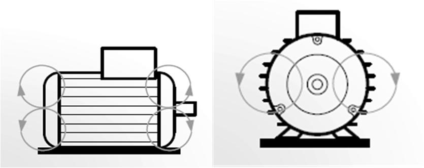
From a physical point of view, an external magnetic field appears in the vicinity of an electrical machine because the internal magnetic field is not perfectly channeled by the ferromagnetic parts of the machine. This external magnetic field can be decomposed in transverse and axial components. The axial field is in a plane that contains the machine axis. It is generated by the winding overhang effects. The transverse field is located in a perpendicular plane to the machine axis. It is an image of the airgap flux density b which is attenuated by the stator magnetic circuit. Figure 1.1 shows a simplified representation of both fields.
Figure 1.1. (a) Axial field. (b) Radial field
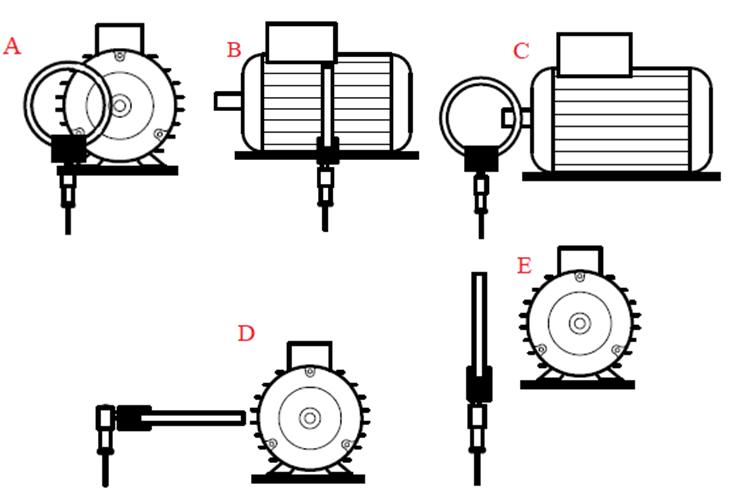
Using a simple wound sensor, it is possible to discriminate the transverse component from the axial component. Figure 1.2 shows different positions of a wound sensor around the machine.
In position A, only the axial field is measured. Position E, although defined as being a position for measuring the transverse field, can also embrace a part of the axial field depending on whether the sensor is more or less distant from the end coils. Position D is described as “pure radial” since, in theory, no axial line field can cross the section of the sensor in this position. It should be pointed out that the amplitude of the signal delivered by the sensor in positions B and D are generally lower. Actually, in these positions, the sensor is further away from the motor compared to position E where the sensor is pressed against the external frame. It is, therefore, possible to define the ideal position of the sensor that it is placed against the motor, in the center to limit the end coil effect, and when possible at design, between the stator sheets and the external frame. In this position, the sensor mainly measures the transverse field. However, practically, the sensor setting depends on the construction of the machine, its environment and the accessibility places.
In the following sections, only the transverse field will be considered and particularly its normal component that requires us to define an attenuation coefficient that affects the airgap flux density.
Figure 1.2. Different sensor positions
1.2.2. Attenuation of the transverse field
Let us define the airgap flux density as the following double sum expression:
where bK,H is an elementary flux density component defined as
with K being the frequency rank and H the pole pair number of the component.
Figure 1.3 shows a simplified representation of an electrical machine, with smooth airgap, where the main dimensions are presented. The external transverse field can be itself decomposed in a normal component bn and a tangential component bt. An elementary component generated in the airgap of the machine is attenuated across the stator yoke and is found in the air outside the machine and can be measured by a coil flux sensor.
Figure 1.3. Simplified geometry of the machine
An attenuation coefficient CH is defined as the ratio between the magnitude of the normal component of the transverse filed at the level of the external periphery of the stator and the magnitude of the component in the airgap. This attenuation coefficient depends on the inner and the outer radii of the stator laminations, respectively, denoted by s intR and s extR , and the magnetic permeability r [ROM 09]. It has been shown that CH can be expressed as
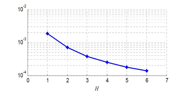
Figure 1.4 shows the evolution of CH versus H for s int 82.5mm R , s ext 121mm R and r = 1,000. We can observe that the more H increases, the more the components are attenuated.
1.2.3. Measurement of the transverse field
We will assume that the measurement is performed with a wound flux sensor placed very closely to the stator core such that only the CH attenuation coefficient will be considered. Let bx denotes the normal transverse flux density at radius s extxR . Here bx is defined by
Figure 1.4. CH versus H
Let introduce x bK the harmonic of K rank of bx at the given point M ( s ext x R , ss 0 ), corresponding to the center of the wound flux sensor. x bK can be defined by
where ˆ xbK can be computed by introducing complex quantities:
The measurements are performed with a coil flux sensor constituted of an n c turn coil (see Figure 1.3) of area S. The angular frequency flux K linked by the sensor results from integration of x bK on S:
The integration depends on the sensor shape, the n c value, S, H and x. By introducing these parameters in the coefficient x H K , x K is given by
Among the components which constitute x K , only few of them, relative to low pole number (low H), have a significant contribution, whereas the other components will be absorbed by the ferromagnetic parts of the machine. The induced emf e x delivered by the sensor is given by
1.2.4. Modeling a healthy machine
The airgap flux density b results from the product between the airgap permeance and the magneto-motive force (mmf) . The following analytical developments consider a general case relating to a p pole pair AM.
To determine the airgap flux density b, the following assumptions are formulated:
– the magnetic permeability of the iron is high enough to neglect the ampere-turns consumed in the iron compared to those in the airgap, – the stator inter-turn short circuit only affects the stator flux density. Therefore, even for the healthy machine, we will focus only on the flux density components generated by the stator.
– the p pole pair three-phase stator winding, made up by diametrical opening coils, is energized by a balanced three-phase system of sinusoidal currents s q i (q=1, 2 or 3) of rms value IS and angular frequency :
Let us define as space references:
– the d s axis which is confounded with the stator phase 1 axis, – the d r axis which corresponds to one tooth axis.
Any point M in the airgap can be located by the variables s in relation to d s and r in relation to d r . The axes d s and d r are distant of .
1.2.4.1.
Airgap permeance
The airgap permeance model is based on rectangular-shaped slots, assuming that the field lines which cross the airgap are radial. As the field lines never join the bottom of the slots, practically, in order to express , the airgap can be modeled considering a fictitious slot with a depth equal to the fifth of their opening and assuming the field lines are radial. In such conditions, can be expressed as
Here, kskr is a permeance coefficient that depends on the slot geometry. N s and N r are, respectively, the number of stator and rotor slots per pole pair. ks and kr are positive, negative or null integers. s is the angular abscissa of any point in the airgap related to the stator referential d s represents the angular position of the rotor tooth 1 axis relatively to d s When the machine rotates R angular frequency, can be expressed as 0 R t . For an SM, R is given by (1)/ R s tp, where s is the slip of the machine.
1.2.4.2.
Healthy machine mmf
The mmf s generated by a healthy stator can be expressed as s s ssssscos(), h h IAthp [1.12] where hs is defined by hs=6k+1, where k varies between to + . s s h A is a function that takes into account the winding coefficient tied to the rank hs .
1.2.4.3.
Airgap flux density
The calculus developments lead to define b= s in the reference frame related to d s as follows:
After regrouping the components of same frequency and same polarity, we obtain
1.2.5. Modeling a faulty machine
For modeling the faulty machine, we will consider a three-phase stator winding. It is supposed that y turns from the n s turns of an elementary section belonging to the phase q are short-circuited. If y is small compared with pn s, the total number of turns per phase, then it is possible to consider that the currents flowing in the three phases remain practically unchanged in faulty conditions. This hypothesis can, therefore, characterize the short circuit, thanks to a model that preserves the original structure of the machine. This model assumes that the stator winding in default is equivalent to the healthy winding, associated with y independent turns in which circulate the short-circuit current. It will be assumed that these two circuits are independent. The healthy part of the winding generates, therefore, the same flux density components without fault.
Figure 1.5. Model of a faulty machine
Figure 1.5 shows an elementary section with short-circuit turns. In this way, the resulting airgap flux density b* is equal to the initial airgap flux density b, to which is added the flux density bsc generated by the y turns flowing through by the current s qsc i : sc bbb .
The short-circuit current is defined as s qscscsc2cos(), iIt [1.17]
where sc is the phase lag between the short-circuit current and the phase 1 current (see Figure 1.6). This phase actually depends on several parameters such as the impedance that limits the short-circuit current, the short-circuit winding, and the position of the fundamental airgap flux density relative to the phase current q (depending on the load).
s qsc i 1 s i sc
Figure 1.6. Diagram of current
The mmf generated by the y short-circuit turns, shifted of from ds, is shown in Figure 1.7 in the case of a four-pole machine. It is also shown the mmf generated by the healthy elementary winding. is an unidirectional mmf and can be decomposed in rotating fields which rotates in the opposite direction. In a stator referential, can be written as
cos(), hh h IAth [1.18]
where s Ah is a function obtained from the Fourier series of s qsc and h is a not null relative integer, which can take consequently all the values of hs . h is defined as s qsc h h .
Figure 1.7. mmf generated by the faulty turns
As s scqsc b , the calculus developments lead us to define this quantity in the reference frame related to ds. After regrouping the components of same frequency and same polarity, we obtain
ks and kr are equivalent to ks and kr, respectively, where they vary from to + . The resultant flux density appears, after attenuation, at the level of the external transverse field.
Considering the values that K can take as given by [1.16] and Ksc by [1.20], it results that Ksc does not bring new frequencies. This means that with the traditional method of diagnosis, the presence of failure will be appreciated through the variation of the amplitudes of already existing lines in the spectrum. This makes the diagnosis by analysis of the changes in the amplitudes of the measured components difficult.
Concerning the polarities H and Hsc, we can observe that Hsc can take all positive and negative integers, whereas H is multiple of p. Hsc can particularly be equal to 1 corresponding to components that are weakly attenuated by the stator iron. In the following, the properties relating to the dissymmetry generated by such components will be exploited.
1.2.6. Effect of the load
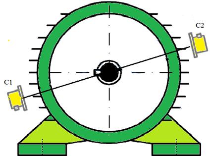
The analysis concerns the behavior, when the load varies, of the amplitude of the sensitive harmonic of rank Ksc measured using two sensors C1 and C2 shifted by 180° with respect to each other to a radius x from the axis of the machine (as shown in Figure 1.8). To simplify the analysis, we will consider the main effects generated by the components having the lowest polarities, namely of polarity p (H = 1) for the healthy machine and with polarity Hsc = 1 for the components generated by the fault. These low polarities lead to the lowest attenuation of the flux density components through the stator laminations.
Figure 1.8. Positioning of two coil sensors. For a color version of the figures in this book, see www.iste.co.uk/soualhi/electrical2.zip
For both positions: 0 (position 1 for sensor C1) and (position 2 for sensor C2), the flux density components • and • of rank K = Ksc can be expressed as the sum of a term relative to the healthy machine of amplitude and a term related to the faulty turns of amplitude , :
Position 1:
Position 2:
1
2
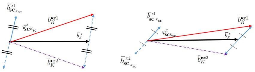
The only change between positions 1 and 2 is the change in the sign of the faulty term. This is due to the polarity Hsc=1 that changes the sign of the cosinus (cos( )= cos( )). The vector diagram for the rank K harmonic associated with a variation of the load is given in Figure 1.9 (in this diagram, we take ∅ 0). To make this diagram, it is considered that the current of the short-circuit part is modified in phase when the load varies, which leads to a change in the phase of the flux density bsc generated by the short circuit and consequently the sensitive harmonics of rank Ksc. The load variation also modifies the flux density coming from the healthy part of the machine because of the increase in the in-line current
We can observe several properties concerning the harmonic of rank K. First, we note that the amplitudes of the resulting complex quantities • and • are different in the presence of a fault (except in the case where ∅ , would be close to /2). For the healthy machine, as the faulty component , does not exist, then the amplitude of the harmonic should remain identical all around the machine. This property related to the difference in amplitude can be used for the detection of an inter-turn shortcircuit fault. However, the magnetic attenuation effects that are in theory independent of the position around the machine can disturb the analysis based on this property. Indeed, practically, structural asymmetries due to the presence of ferromagnetic parts in the environment close to the machine will possibly lead to a non-uniform attenuation of the flux density according to the angular position. It will thus be possible to obtain different amplitudes even in the case of a healthy machine. Nevertheless, in this case, the amplitudes • and • , even different, will at least evolve in the same direction as load variations.
To overcome this problem, we can exploit the behavior of the sensitive harmonics in the case of load variation. We can see in Figure 1.9 that a load variation, which induces a change in , and ∅ (and consequently ∅ , ), will lead to a difference in the amplitude variation between • and • . This difference in amplitude variation is likely to change when the load varies.
Actually, the positioning of the sensors regarding the axis of the faulty winding affects the results. Indeed, the best positioning is when the sensors are placed perfectly in the axis of the faulty winding. In this position, the difference in amplitude variation is maximum, and in this case, the
amplitudes may vary in the opposite direction [PUS 10], which is a very reliable indicator of fault.
(a) (b)
Figure 1.9. Phasor diagram variation: (a) load 1; (b) load 2
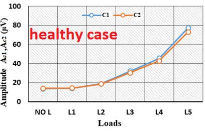
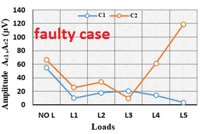
Figure 1.10 shows the variations with the load level of the Ksc rank harmonic of the emf delivered by the two sensors positioned at 180° from each other around an electrical machine. Two cases are presented: the healthy case and the case with a stator inter-turn short-circuit fault. The following observations are consistent with the theoretical analyses:
– in the healthy case, the harmonics vary in the same direction and have in this case almost the same amplitudes;
– in the faulty case, the harmonics vary differently, and sometimes in opposite directions.
These types of curves obtained in different machines can be analyzed from two indicators:
– the ratio of amplitudes (RA), which gives the ratio between the amplitudes of the harmonics measured on both sides of the machine,
– the difference of variation (DV), which is a Boolean quantity: either the harmonics vary in the same direction, or they vary in opposite directions.
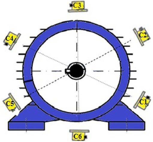
As the detection performance depends on the position of the sensors regarding the localization of the fault in the winding, it is possible to improve the diagnosis using several sensor positions around the machine. The pair-forming sensors will be shifted by π as shown in Figure 1.11, where six sensors are used. However, it will not be possible to cover the entire periphery of the machine, for example, it is not possible to place a sensor under the base of the machine.
1.3. Information fusion to detect the inter-turn short-circuit faults
As shown previously, to improve the reliability of the approach, measurements at several positions will be performed. Each measurement constitutes a piece of information regarding the presence of a fault. Fusion technique [BLO 07, KHA 13] using the belief function theory [DEM 67, SHA 76, SME 94] is used here as a frame to represent and combine information to make a final decision. This theory is a powerful mathematical framework used to deal with partial and unreliable information [DUB 10] in many fields [DEN 16].
Figure 1.10. Variation of sensitive harmonic versus the load
Figure 1.11. Measurements with three pairs of sensors