1 INTRODUCTION
1.1 Introduction
Welcome to our book on calculus.1 We are four mathematics education researchers, but we have clocked-up many decades of practical teaching of calculus at school and university level in Brazil, New Zealand, the United Kingdom and the United States. This book is about teaching calculus, it is not a calculus textbook. This book concerns introductory courses in calculus (elementary calculus) of a sin gle variable, which may be in the latter years of high school or the first year of uni versity, depending on country and/or institution. It is primarily a book for teacher educators, i.e. people who teach teachers, secondly for (school or university) teach ers who wish to know more about ways to introduce their students to calculus and thirdly for people, such as PhD students, who are contemplating doing mathematics education research on an aspect of calculus. This book offers a variety of methods to approach the teaching of calculus, provides a reader-friendly overview of research on the learning and teaching of calculus and presents educational and mathematical mat ters for consideration (Edumatters and Mathematters) at various points in the chapters. There are eight chapters:
1 Introduction
2 Calculus across time and over countries
3* Making sense of limits and continuity
4* Making sense of differentiation
5* Integration and the fundamental theorem of calculus
1 Or ‘analysis’ in some countries. The literature on calculus sometimes writes ‘the calculus’ or ‘Calculus’. We have opted for ‘calculus’ to keep the writing style plain.
DOI: 10.4324/9781003204800-1
6 Interlude: the ordering of Chapters 3, 4 and 5
7* Calculus applications: differential equations and integration
8 Beyond elementary calculus.
The chapters marked with a star (*) address the substance of elementary calculus. We now briefly describe each chapter.
Chapter 1, which you are reading, introduces the book. This introduction is followed by three sections: mathematical prerequisites for the study of calculus, theoretical approaches mentioned in this book and a mathematical overview of dif ferential and infinitesimal calculus. Mathematical prerequisites are important for teaching any course, so we thought we’d put our considerations at the beginning of the book. The section on theoretical approaches is there to help readers who do not work in the field of mathematics education. You can be a brilliant calculus teacher without knowing anything about the social-linguistic theory of commognition, but if we mention, say, a commognitive study on teaching the derivative, we want a quick way for you to find out what the theory of commognition is. The last sec tion provides a mathematical overview of differential and infinitesimal calculus. This overview is needed to fully understand parts of the following chapters as we often present differential and/or infinitesimal ways to understand calculus ideas.
Chapter 2 has two sections: a brief account of the history of calculus and a brief account of calculus around the world. Both sections could be books in themselves, so there is a need to focus on what is needed for the rest of the book. The history of calculus section outlines major landmarks from Archimedes to Leibniz and Newton to the arithmetisation of calculus in the 19th century to the invention of nonstandard analysis in the 20th century. The calculus around the world section considers school and beginning university calculus curricula from a number of countries. The approach is synchronic not diachronic; it would be nice to present the development of calculus curricula over time, but this is unrealistic given the length of the book.
Chapter 3 has four sections. The first looks at the place of limits and continuity in elementary calculus curricula and one well know curriculum, Advanced Placement Cal culus, in particular. The second section provides an overview of education research on limits and continuity. This is followed by a short history of limits and continuity. This history is important in understanding that limits have not always been a part of calcu lus and that continuity was a central construct in the early days of calculus. The final section looks at ways that limits and continuity can be introduced in your classroom.
Chapter 4 presents ways that (parts of) a first course in differential calculus can be taught and learnt meaningfully. It does not tell you how to teach differentiation but, rather, presents you with different ways to do this. The chapter discusses prior knowledge and curricula matters, ways that differentiation can be introduced, the rules for differentiation, special functions, what derivatives tell us about functions and their graphs, tasks and an overview of education research on differentiation.
Chapter 5 presents the main ideas of integral calculus and the fundamental theorem of calculus (FTC). The focus is on significant mathematical and conceptual elements involved in making sense of these ideas. Different approaches to teaching integration
and the FTC are presented along with notes on the pros and cons of these approaches. Throughout the chapter, descriptions of research about student reasoning with integrals and the FTC are presented to augment the discussion of concepts and ways of teaching.
Chapter 6 considers, and questions, the classic ordering of a first calculus course: limits, differentiation and integration. It is a very short chapter, an interlude that reflects on the previous three chapters.
Chapter 7 discusses some applications of calculus to real-world problems such as the spread of viral infections and simple harmonic motion. It begins with a consideration of first and second order ordinary differential equations and covers the nature of their solu tions as functions, how these may be approximated and their graphical representation us ing slope fields. There is also an overview of educational research on differential equations. The second part of the chapter looks at applications of integration that involve finding volumes of revolution, surface area and lengths of curves. Finally, some methods of ap proximating the values of integrals are considered with applications such as ship stability.
Chapter 8 considers aspects of calculus and/or real analysis courses that come after an elementary course in calculus. It does not attempt to describe the content of these courses but raises matters that teachers of elementary calculus should, in our opinion, note with regard to what calculus related things their students may do (or not!) in their future studies.
1.2 Mathematical prerequisites for the study of calculus
It could be argued that, apart from giving them practical arithmetic skills, one of the primary purposes of the secondary mathematics curriculum is to prepare students for the study of calculus. In which case, describing the prerequisites for the study of calculus ought to be easy. However, our goal here is not to give a list of school mathematics topics, such as arithmetic techniques, that would have little value in this context but rather to try to say what are some key constructs that will contribute to student understanding of calculus.
In the preceding sentence, we have deliberately avoided use of the word ‘skills’ in favour of constructs, whatever they are. We should explain why. One way to divide mathematics content is into skills and processes, and another way to divide math ematics content is into objects, concepts and constructs. Of course, these two groups are not totally disjoint but are related in a fundamental way, which will be explained in Section 1.3 of this chapter. Suffice it to say at this point that mathematical pro cesses can undergo a cognitive encapsulation into mathematical objects (Dubinsky & McDonald, 2001; Tall et al., 2000). We would argue, with the support of consider able research evidence (see, for example, Kieran, 2007, and the review of Rakes et al., 2010) that there has been, in many countries, a greater emphasis on the former than on the latter. For example, students may be able to add or multiply decimals without really understanding the concept of place value or be able to factorise bino mials without understanding what factors or quadratic functions are.
Hence, in the main we will place an emphasis here on what objects, concepts and constructs students would be well advised to understand in order to do well in
calculus. Occasionally we may also mention a skill or process that would also help. It will be difficult to present them in the order that would usually be met in school since this will vary from country to country, and even within countries, from school to school. In addition, the approach employed and the level of formality or rigour used will also vary considerably. So the key point is that they need to be understood in the context of what that may mean in the local curriculum.
1.2.1 Important mathematical constructs
1.2.1.1
Number
Clearly the concept of number underpins much of mathematics, and while the set of real numbers as a complete ordered field and the corresponding real number line will be a step too far for the vast majority of secondary school students, some idea of the relationships between sets of numbers and how they might be represented will be of benefit. Further, representing these using both interval and set notation is recommended. So, for example, there is value in having the sets = {12 3,.} ,, , =. 321 01 23,,,, and relationships N ⊂ Z ⊂ Q ⊂ R { ,, . (without needing a formal definition of ), along with interval notation, ( --, 1] = {x : x E Rx : 1}, , x [– 1, 3), and so on. A good understanding of proportionality will be beneficial along 111 with some basic familiarity with convergent sequences (e.g. that 1,, , , . . . gets 248 nearer and nearer to 0).
1.2.1.2
Variable
We have known for a number of years that many students’ understanding of letter or symbolic literal use in algebra does not extend to generalised number or variable (Küchemann, 1981). This may be because greater emphasis is placed in classrooms on the use of variables rather than on understanding what they are or that many school texts are silent on the definition of a variable. A key part of the difficulty here is to know what kind of definition to give to students. For example, both Schoenfeld and Arcavi (1988) and Wagner (1981) give a number of possible examples of symbol usage in mathematical statements.
We would, of course, expect variables to vary, but describing the manner in which they do is not so straightforward. Skemp (1979) says “In mathematics, an unspecified element of a given set is called a variable” (p. 228). So the statement ‘Let x ∈ ’ is used in this way to say that x is an unspecified real number. However, this can appear to be a rather static idea that says nothing about exactly how x might vary. Thompson and Harel (2021) stress the point that in order to understand both rate of change and accumulation, two fundamental ideas in calculus, students need to be conversant with the process of covarying two quantities. Addressing the thought of how variables vary, they are unconvinced by the idea that it means replacing one value with another. Instead they espouse the construct of ‘smooth variation’ and
say that “If calculus students are to understand something akin to instantaneous rate of change, they must envision that smooth variation happens in bits” (ibid, p. 512). Thus, students would benefit from experiencing quantities that do indeed vary. For example, if a conical container is filling with water such that the height of the water in the container is given by x and the corresponding volume by V(x) then V varies simultaneously with x, and it is this covariation that can provide valuable experience (Thompson & Harel, 2021). Assisting students to see, for example, the smooth vari ation of the height quantity from x to x + h as the volume varies smoothly from V(x) to V(x + h) and representing these on Cartesian axes as a continuous graph can help build understanding in preparation for calculus. Other examples that could prove useful are to think of how variables change over time. If students are familiar with basic kinematics (formulas and graphs linking distance, velocity, acceleration and average velocity), then this can also be useful for seeing this kind of variation, as well as providing good applications for later differentiation and integration. For example, if a velocity is changing with respect to time, then we may have
Vt() = 30 + 10t
and, if δt is a small change in t, and the corresponding small change in V is δV , then
V + 8V = 30 + 10 ( t + 8t ) So
8V = 108t
1.2.1.3 Function
Of course, we have already used function notation in the previous section, and we stress the point that what is provided is not an intended order for studying these concepts and neither should they be thought of as disjoint entities, but rather there is some overlap between them. While function is a fundamental concept of mathemat ics, there is a tendency, as with variable, for it to be used in many school classrooms without being defined. As a consequence many students may think of a function as an equation, a graph or an input-output process rather than as a correspondence, a mapping, a set of ordered pairs or a rule (Williams, 1998). This leads to erroneous ideas such as a function must have a formula, its graph needs to be smooth and con tinuous, or even that due to stressing the vertical line test, the graph, rather than any algebra, is the function (Thomas, 2003). In addition, often student experiences with functions, and their graphs, has been limited to construction of pointwise and global perspectives (Vandebrouck, 2011). Hence, they may evaluate the value of a function at a specific point, finding fa , say, deal with a function globally or on an inter () val by translating its graph or finding its concavity, but they rarely consider a local
perspective that involves small intervals such as [ xh, xh + ] (Thomas et al., 2017), where the behaviour of the function on small intervals of decreasing size is a focus. This becomes important for a study of, for example, when a function is continuous. Working with functions is also important in calculus. We mention just a few key aspects of this here. One is that a working understanding of simple polynomial func tions (linear, quadratic and cubic) and their Cartesian graphs seems essential, along with the concept of gradient (or slope) and its application to linear functions (e.g. an ability to identify positive and negative gradients and to ascribe approximate nu merical values to the gradients) and estimating gradients of quadratic functions using tangents. It is important to define a polynomial (function) since research has shown that a number of students do not think of examples such as 05 2x + 1 ,, as polynomials -1 + (since, they may reason, poly means greater than 1) but may also think that xx is one.
Another important concept is the domain of a function, the values of the inde pendent variable for which the function is defined. This becomes important when thinking about differentiating functions given by a formula such as fx = ln gx ) () ( () , in order to consider when g(x) might be zero or negative, and hence f is not defined, 1 as well as thinking about the values of x for which functions such as y = can be x integrated. We note in passing that both notations, y =. and fx() =. will be of value in different areas of calculus2 and so making students familiar with both is a good idea (see Chapter 2 for historical information on why both are used). Know ing and understanding a wide range of different functions is also valuable. Some other examples include trigonometric, rational, exponential and power functions. See Section 4.2.5 for a fuller discussion of some of these functions.
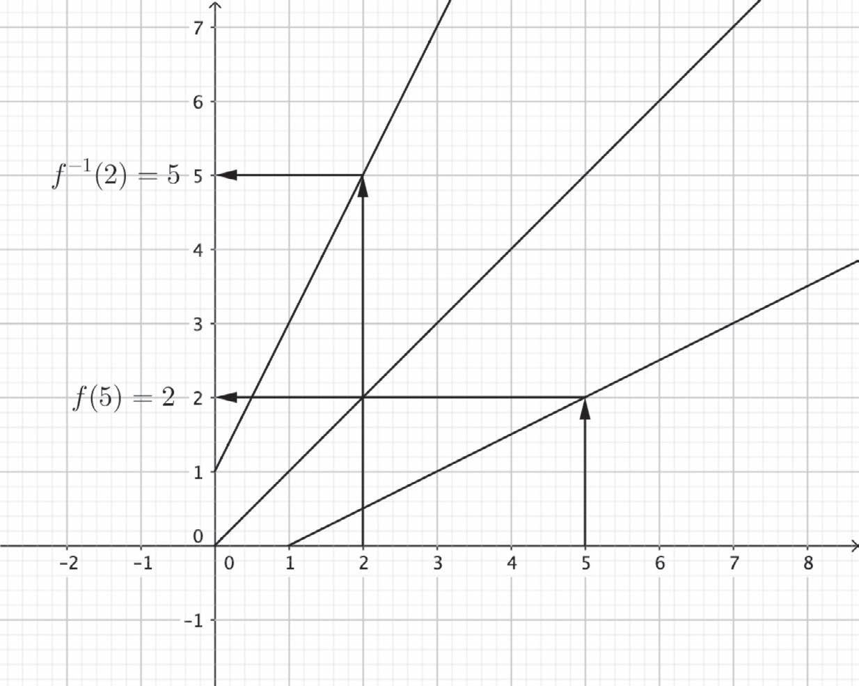
A second consideration is the concept of an inverse function and when it exists. This is when the function, possibly on a restricted domain, is 1–1 (injective) and onto (surjective), also called a bijection. In this case if y f x then x = f y = () -1 (), when it exists. This, of course, is why the standard process for finding an inverse function, to make x the subject of the equation, works. Students may be taught that the graphs of a function and its inverse are symmetric about the line y = x (see Figure 1.1). If this is used then it is important, of course, to stress that this is only the case if the x- and y-axes have the same scales.
A third useful idea is that of composition of functions, and this is best accom plished with the fx , written fg can () notation. A composite function of f and g be defined3 as
fg x ) () = f gx ) ( ( ()
2 It is worth noting here that we should use, say, f as the notation to represent a function, whereas f(x). is the value of the function f at some point x. 3 gf is also a composite function.
FIGURE 1.1 Illustrating the relationship between fa a () and f -1 ()
providing we also make sure that the domain of f contains the range of g so that fg x () is defined. Then the domain of fg is the domain of g () (or a subset of it) and the range of fg is a subset of (or equal to) the range of f. It is worth not ing that although real functions are strictly defined between two given sets (such as f :\ 0 {} - ) it is common practice in mathematics to give a rule for a function and assume that the (natural) domain is the largest subset of the real numbers for which the function is defined. Thus, instead of, say,
h :, 4 o ) - [ defined such that
hx = x - 4 () we will often be given just
hx() = x - 4 without the domain information, and we have to supply this ourselves. This makes the composition of functions trickier. For example, we might ask whether our
students could say what the natural domains would be for the functions fg and gf where ( 2x - 1)2 fx = () x + 1 and 2x - 1 gx() =
8 Introduction x - 1 2 .
In addition, it may also be useful if students have some experience working with the binomial theorem, but it is possible to introduce this topic/concept during the study of differentiation.
1.2.1.4 Geometry
An understanding of geometrical concepts can be very useful in calculus. One important example is the measurement of angles using radians (see also Section 4.4). If we define a radian to be the angle subtended at the centre of a unit circle by an arc 2n of unit length, then since the circumference of a unit circle is 2π.1 there are = 2n 1 radians in a circle. Thus 2π radians are equal to 360˚, and so, dividing by 2 and using c to represent radians,
t c = 180 . and ° 180 c = 1 n or n c 1 o = . 180
Thus the length of an arc subtending an angle of θc at the centre of a circle of radius r is e n = e • 2 rr 2n
And the corresponding area of the sector is e 2 1 2 • n r = r e 2n 2
These ideas become essential when we start to differentiate trigonometric functions such as fx = x and gx = x in order for the answers to be easier () sin () () cos () functions, since, for example fx ' º = cos x º () when x () () , rather than cos x is 180
t
in radians. This is because the limit arising in the formal definition of derivative (see Chapter 4)
( h ( sin || ( 2 ) #
lim = h ->0 ( h ( 180 || ( 2 ) when h is measured in degrees, but 1 when h is in radians.
Mathematter
Questions to ponder – concepts versus procedures
(i) A cylinder has radius r and height h, while a sphere has radius r. If the radius of each is increasing at the same rate, which is increasing faster, the volume of the cylinder or the surface area of the sphere? Explain.
(ii) Why should a student think about before they begin a process to solve
23 64 1 x x + + = ?
If they go ahead and use a procedure to ‘solve’ it, what would you say to them about the answer x =-15.?
(iii) Which of these do your students think are equations?
yx=+21, 93 6 =+ , 23 25xx() =, ab ab -+ - 35 8 , 31 33xx + () =+
What reasons can you think of for why they may think that way?
(iv) Which of these represent functions? Which polynomials? Why or why not?
a) y x =1 1 b) ht() = # c) 23 5 2 xy x +- = d) pm m () =( ( | ) ) | -sin 1 4 #
(v) If 21 0 x -= and 31 0 x += then 2131 xx -= + , since both are equal to 0, and hence x =-2. How would you discuss this reasoning with a student?
(vi) How would we get students to solve these equations?
a) (i) 25 9 x -= (ii) 23 59 x + () -= b) (i) 25 72 1 22xx xx=+ + (ii) 27 61 22xx xx=+ +
(vii) Does the function ff xx :,12 1 2 () -> () =-() R where have a maximum value?
1.3 Theoretical approaches mentioned in this book
As part of the IMPACT series of books, this book aims to integrate mathemat ics content teaching with the broader research and theoretical base of mathematics education. In particular we refer, at times, to approaches and ideas current in math ematics education research. We are aware that some readers will not be familiar with these. This section is written to provide such readers with an overview of approaches and ideas we mention. Our overview errs on the side of brevity; fuller descriptions of approaches and ideas are available in the Encyclopedia of Mathematics Education (EME, https://link.springer.com/referencework/10.1007/978-94-007-4978-8)
We start with constructivism 4 This is a theory of knowledge development that emerged, alongside other influences, from Jean Piaget’s developmental psychology. Piaget considered knowledge as cumulative and cognitive development as mov ing through four stages: sensorimotor (0 to 2 years), preoperational (2 to 7 years), concrete operational (7 to 11 years) and formal operational (12+ years). He posited, amongst other things, three constructs in cognitive development:
• Schemas – cognitive structures representing a person’s knowledge about some entity or situation, including its qualities and the relationships between these5
• Assimilation – fitting new information into existing schemas, e.g. negative numbers
• Accommodation – modification of existing schemas in the light of new informa tion assimilated.
Constructivist mathematics educators apply these constructs to all aspects of learn ers’ mathematical development. For example, Taback (1975) found that, at each Piagetian stage, limit-related schemas held by the children were inherently contra dictory. In the late 20th century, two versions of constructivism emerged: radical constructivism, cognition is the sole driver of knowledge development; and social constructivism, the cultural-historical development of knowledge precedes individual knowledge development.
Social cultural (socio-cultural) approaches, including social constructivism and activity theory,6 view individual knowledge development within social structures, historical development and the use of language and tools. Many social culturalists subscribe to Vygotsky’s (1978, p. 57) statement, “Every function in the child’s cul tural development appears twice: first, on the social level, and later, on the individual level; first between people . . . then inside the child”. The context of learning is not a side issue for social culturalists as the who with, where, with what (tools) and why of learning cannot be separated from the learning itself. For example, mathematics done by a student using a computer algebra system (CAS) cannot, for a social cultur alist, be reduced to what the student alone can do or to what the CAS can do; the
4 EME: Constructivism in Mathematics Education
5 https://dictionary.apa.org/schema
6 EME: Activity Theory in Mathematics Education
mathematics is done by the student-with-CAS. Bingolbali and Monaghan (2008) is an example of a social cultural study on derivatives as it views students’ understandings through students’ positional identities as engineers or as mathematicians.
Realistic Mathematics Education7 (RME) is an approach to the design of teaching mathematics that emerged in the Netherlands in the 1970s and is still developing. The word ‘realistic’in the title does relate to real-world situations, but it is also intended to convey that the mathematical teaching sequences designed should connect with the real-life experiences and imaginations of the students by offering them problem situ ations for the guided reinvention of mathematics. The word ‘mathematising’ was coined by RME didacticians to emphasise the verb of doing mathematics rather than just learning facts. RME distinguishes between horizontal and vertical mathematisations. The former involves mathematising extra-mathematical phenomena from the real world. Vertical mathematisation is inter-mathematical and involves building new (for the student at a particular stage in their mathematical development) mathematical connections between prior knowledge. RME has strong links with (and influenced the development of) design research and stresses: starting from problems which are meaningful to students, learning by doing and gradual mathematisation.
The Anthropological Theory of the Didactic8 (ATD) was initiated by Yves Chevallard in the 1980s and focuses on institutional aspects of mathematics education. A central construct is the didactical transposition which traces the movement, over institutions, of scholarly knowledge (produced by mathematicians, e.g. the limit notion) to curricula knowledge (knowledge to be taught) to knowledge taught and knowledge learnt (by stu dents). ATD posits two knowledge blocks praxis and logos. Praxis consists of tasks and techniques (e.g. integration by parts) to solve the tasks. Logos concerns the underlying rationale for the praxis and has two levels: technology, which concerns the discourse used in describing techniques; and theory, which provides the basis for the techno logical discourse. The theory is supposed to justify the technology by linking histori cally accumulated mathematical knowledge to knowledge taught but ATD analyses often show that this linkage is often nebulous. For example, in an ATD study of limits at high school, Barbé et al. (2005) reveal constraints that significantly determine the teacher’s practice and the mathematics taught. The development of ATD is ongoing but the aforementioned description suffices for references to ATD in this book.
Commognition9 is a word made from the words ‘communication’ and ‘cogni tion’ and is a socio-cultural approach which views cognition and communication as two sides of the same coin: thinking is communication with oneself, and learning mathematics is participation in mathematical communication. Discourses are types of communication which include words (e.g. functions); visual mediators (e.g. graphs); narratives, stories about the objects of the discourse and routines, repetitive patterns in the discourse. Routines in mathematics classes include explorations aimed at endorsing narratives, deeds which involve practical action and rituals which are things done to
7 EME: Realistic Mathematics Education
8 EME: Anthropological Theory of the Didactic
9 EME: Commognition
create a common purpose in mathematics lessons (e.g. algebraic actions to establish a point of inflection). Commognition views learning as ‘change in discourse’ which can occur at the object-level or the meta-level. At the object-level, change concerns the logical development of previously endorsed narratives of the discourse. At the meta-level, learning change does not follow logically from previously endorsed nar ratives but involves discursants (participants) making choices. Commognitive research on the teaching of learning of calculus thus pays close attention to what is said and done in classrooms with respect to the many constructs it introduces.
Embodied cognition10 is a branch of cognitive psychology, but in mathematics edu cation it represents a view that learning mathematics is a mind-body activity, not just a mental act. This is not a new idea, but embodied cognition is a relatively new term (late 20th century). This is easy to appreciate in elementary mathematics – a child using her fingers to count – but is it relevant to higher mathematics, calculus in particular? Carry out the following thought experiment: you are observing a student teacher teaching a first lesson on the derivative and introducing the gradient of the tangent to a function at a point – does the student teacher put her hand to graph at the point and incline the hand in the direction of the tangent at the point? Probably. There are now many different views on the extent and importance of embodied cognition but reference to it in this book will keep to this basic idea.
Before introducing the next two theoretical approaches, we introduce the phrase/ construct, process-object encapsulation, which refers to making an object out of a pro cess. For example, the teaching and learning of functions usually begins with an input-output process, e.g.
1014
() 4
Students usually need to spend a considerable amount of time before this concep tion moves to viewing fx() as a single entity, an object. Process-object encapsula tion permeates much of school mathematics number and algebra curriculum. Gray and Tall (1994) introduce the term ‘procept’ (process-concept) for process-object encapsulations where the student can move back and forth between process and object conceptions.
Actions, Processes, Objects, Schemas (APOS)11 is a branch of constructivism which embraces process-object encapsulation. Schemas are the end-point in learning a con cept, which starts with actions and moves to processes and then to objects and finally schemas for the concept. Students are not always successful in reaching object or schema conceptions. APOS is used widely in studies of advanced mathematics. Asiala et al. (2001) is an example of an APOS study on students’ graphical under standings of the derivative.
David Tall (with others) developed the metaphor of the three worlds of mathematics and has brought this into many accounts of learning calculus (Tall, 2013). The three
10 EME: Embodied Cognition
11 EME: Actions, Processes, Objects, Schemas (APOS) in Mathematics Education
worlds are: an embodied world, a symbolic world (developed from the embod ied world) of actions into symbolic procedures (procepts) and a formal (axiomatic) world where concepts are defined and their properties are deduced. He views these three worlds as developing over time in the life of an individual and in the history of mathematics.
1.3.1 Teacher knowledge12
An import construct, pedagogical content knowledge (PCK), in teacher education was introduced in Shulman (1986, p. 8). Good teachers, he argued, must not only possess content knowledge and pedagogical knowledge; there must be interaction (intersection in terms of Venn diagrams) between these two forms of knowledge –pedagogical content knowledge. In the field of mathematics education this idea was refined, by D. Ball and H. Bass (2002), to mathematical knowledge for teaching (MKT). They sub-divide content (mathematical) knowledge into ‘common’, ‘specialised’ and ‘horizon’ content knowledge. Common content knowledge is required by everyone; specialised content knowledge is unique to mathematics teaching; horizon content knowledge is knowledge that would benefit teaching but may not be taught because it is beyond the level being taught. The topology of the real number line is an exam ple of horizon content knowledge in the teaching of calculus at the school level.
We end this section with a short account of conversions and treatments of math ematical representations, e.g. algebraic, graphic and numeric forms of a mathemati cal construct such as the derivative. The following does not present a theoretical approach but introduces two constructs used in mathematics education research. A seminal work on representations in mathematics is Duval (2006) where the difference between conversions and treatments is considered. “Treatments are transformations of representations that happen within the same register”13 (ibid., p. 111), for example, changing yx 10 to yx 1. “Conversions are transformations of representa = =+ tion that consist of changing a register without changing the objects being denoted” (ibid., p. 112), for example, changing yx 1 to a Cartesian graph. Duval (ibid.) =+ goes on to note “Conversion is more complex than treatment because any change of register first requires recognition of the same represented object between two rep resentations whose contents have very often nothing in common”. In the following chapters of this book, we often note that multiple representations are important for learning calculus, but Duval’s conversion/treatment distinction reminds us that alter native representations of the objects of calculus also add a level of difficulty.
1.4 A mathematical overview of differential and infinitesimal calculus
When it was developed in the 17th century, calculus was ‘the infinitesimal calculus,’ –a set of methods for working with infinitesimal quantities. In the 19th century,
12 EME: Subject Matter Knowledge Within “Mathematical Knowledge for Teaching”
13 Duval (2006) defines ‘registers’ as semiotic systems that permit a transformation of representations.
infinitesimals were jettisoned from the subject because they were seen to be not rigorously defined, and calculus was reconceptualised in terms of limits. Calculus classes followed suit, and today the vast majority of classes avoid infinitesimals and instead use limits when defining the principal ideas of calculus such as derivatives, integrals and continuity. In the 1960s, Abraham Robinson developed the field of nonstandard analysis (Robinson, 1966), which allows infinitesimals to be formally defined and for calculus to be conducted rigorously using them. He also proved that essentially all the same things can be done with infinitesimal calculus as with limitsbased calculus. Some calculus classes around the globe now use infinitesimals, and some researchers have argued for the benefits of such approaches (for a survey, see Ely, 2021). One potential benefit is that notations originally invented with infini tesimals in mind can more directly refer to quantities, rather than serving as token dy short hands for limit processes. Using infinitesimals, dx has meaning on its own, b dx really is a quotient of small differences, and fx dx f () really is a sum of little bits.
We refer to infinitesimal approaches periodically in this book, since one of our goals is to stimulate the reader to conceptualise familiar elements of calculus in multiple ways and with multiple meanings. The purpose of this section is to provide some technical background for such references and to describe how infinitesimals can be rigorously defined in such a way that calculus can be performed using them. Of course, an infinitesimals-based calculus course need not formalise infinitesimals at all, just as a standard calculus course need not formalise limits with the epsilondelta definition. This section summarises the conceptual basis of such a formalisa tion, based on Keisler’s (1976) treatment, which should be consulted for further details, and which, at the time of this book’s publication, is available online for free on https://people.math.wisc.edu/~keisler/calc.html.
Robinson’s development of nonstandard analysis is one way of formalising Leib nizian infinitesimals. It allows one to imagine a continuum where it is possible to ‘zoom in’ infinitely to reveal differences between points that at a finite scale appear identical. This continuum, the hyperreal numbers, is an extension of the real num ber line, and nonstandard analysis is the theory that works with this continuum. By saying that nonstandard analysis ‘formalises’ the idea of infinitesimal quantities, we mean that it grounds these in the regular ZFC axiomatisation of modern math ematics. Robinson proved the transfer principle, that all (first-order logical) theo rems true in the hyperreal numbers (* ) are true in and vice versa, which means that standard analysis and nonstandard analysis are equivalent in scope, consistency and power. This actually allows current-day mathematicians to pursue results in * or , whichever they find handier, without sacrificing rigour. For instance, Terence Tao uses nonstandard analysis to avoid excessively complicated manage ment of epsilons, and he notes that “non-standard analysis is not a totally ‘alien’ piece of mathematics”, but is “basically only ‘one ultrafilter away’ from standard analysis” (2007). Shortly we shall see what Tao means by “ultrafilter”.
The image Robinson provides us for extending the reals to the hyperreals is to start by picturing an infinitesimal hyperreal number as a sequence of real numbers that converges to 0. Sequences that converge faster to 0 are imagined to be smaller infinitesimals than those that converge slower. Thus we get an array of infinitesimals and comparing them amounts to comparing sequences of reals. The first technicality is that we ought to view the two sequences {1, ½, ¼, 1/8, . . ., 1/2n . . .} and {3, ½, ¼, 1/8, . . ., 1/2n . . .} as the same hyperreal number, since they both converge to 0 the same way. So Robinson begins by describing a hyperreal number not as a sequence but as an equivalence class of sequences of real numbers. The idea is to consider two sequences to be equivalent, (a n) ~ (b n), if a n = b n for “most” indices n. Likewise, we want (a n) > (b n) if a n > b n for “most” n. But how do we know what “most” means? In other words, how can we decide if an index set S = {n: a n = b n} or Q = {n: a n > b n} is “large”?
One criterion for sets to be “large” is that it should allow the relation = (or >) to be transitive. We want (a ) ~ (b ) and (b ) ~ (c ) to imply (a ) ~ (c). Thus, if S = nn nn nn {n: a n = b n} is large, and T = {n: b n = c n} is large, then we need S∩T to be large too, because it might be that a n = c n only for indices n∈S∩T. A second criterion for large sets is that for any set P, exactly one of P or \P should be large. This is because we want (a ) = (b ) when P = {n: a = b } is large, and we want (a ) ≠ (b ) when Q = nn nn nn {n: a n ≠ b n} is large. Two more straightforward criteria for “largeness”: is large and ∅ is not, and if A is large and A ⊆ B, then B is large. An ultrafilter is a collection of subsets of that satisfy these four criteria for largeness. In other words, an ultrafilter is a collection of “large” sets of indices n, and on any of these index sets it is possible to coherently compare two sequences a n = b n .
In order to define the hyperreal numbers, we need to pick an ultrafilter that meets an additional criterion to make sure the hyperreals do not end up being exactly the same as the reals: the ultrafilter must be nonprincipal. This means that every finite set is small and every cofinite set is large. Proving that a nonprincipal ultrafilter even exists requires the axiom of choice, and ‘picking’ such an ultrafilter is a non-constructive endeavour. Nonetheless, this enables the hyperreals to be de fined as follows: fix a nonprincipal ultrafilter. Let R N be the set of all sequences of real numbers and say (a ) ~ (b ) if {n: a = b } is large. The hyperreals are the set of nn nn equivalence classes * = R N /∼
The hyperreals are an extension of the reals, since we can identify any real number r with the sequence {r, r, r, . . .}. It is worth checking that there indeed exist some infinitesimal hyperreals that are not just 0. Consider ε = {1, 1/2, 1/3, 1/4, . . .}. This hyperreal number ε < 1/k for any integer k, because the set S of indices on which {1, 1/2, 1/3, 1/4, . . .} < {1/k, 1/k, 1/k, . . .} is cofinite, hence large. But ε > 0, since the set of indices for which {1, 1/2, 1/3, 1/4, . . .} > {0, 0, 0, . . .} is , which is large. Likewise, ∂ = {1, 1/2, 1/4, 1/8, . . .} is an even smaller infinitesimal, and it is not difficult to show that there are uncountably many more. The reciprocals of all these infinitesimal hyperreals are all infinite numbers, which are also hyperreal.
An operation on real numbers has its analogue in * by just performing the same operation coordinate by coordinate. It can be shown that * is a field under standard arithmetic operations *+ and *×. This means some of the heuristics Leibniz used with infinitesimal and infinite numbers can be proven as theorems in the hyperreals, e.g. “an infinitesimal number times an infinitesimal number is infinitesi mal” and “the reciprocal of an infinitesimal number is infinite”.
In general any statement about real numbers has a ‘starred’ statement for hy perreals, which means that it is true on a ‘large’ set of coordinates. The transfer principle establishes that this relationship goes both ways: a (first-order) statement is true for all real numbers if and only if its starred version is true for all hyperreal numbers. An example is the following statement, which is true in : “For any positive x, there is a natural number n (∈ ) such that x > 1/n”. This sounds like it is not true in * , since there exist infinitesimals there. But the way to ‘star’ this statement is “for any positive (hyper)real x, there is a (hyper)natural number n ( ∈ * ) such that x > 1/ n ”. This is true because * contains infinite numbers. Another very important example is the Archimedean axiom for the real numbers: for any positive a and b, there exists n (∈ ) s.t. na > b. The spirit of this state ment is that a magnitude can always be iterated some number of times to exceed another given magnitude. This statement is not true in the hyperreals, which are a nonarchimedean field. Nonetheless, the statement becomes true when you allow n to be an infinite hypernatural (∈* ).
Using the least upper bound property of the reals, it is not hard to show that each finite hyperreal number p is infinitely close to exactly one real number r. This real r is called the shadow of p (“sh(p)”), or standard part of p (“st(p)”). Likewise, each real number r has a cloud or monad14 of hyperreal numbers that are infinitely close to it. Using ≈ to mean infinitely close, p ≈ st(p). The monad of hyperreals around the real number p formalises the idea that there are numbers that become visible only when you zoom in infinitely on p
When you prove a theorem in the hyperreals, and then ‘unstar’ it to get the corre sponding statement in the reals, this unstarring often entails ‘rounding’ finite hyperreal numbers to their shadow or standard part. For example, consider the function y = x2 in *. Choose an infinitesimal non-zero increment of x, calling it “dx”. We can find the corresponding increment of y, represented as dy, as follows:
dy = xdx 2 x 2 ( + ) - ()
2 2 2
dy = x + 2xdx + dx - x
dy = xdxdx 2 2 +
14 Robinson picked this term as a tribute to Leibniz. For Leibniz, a monad was a fundamental meta physical particle, not a mathematical entity used in calculus.
We can go further if we wish, and divide both sides by the infinitesimal dx, since division works normally in the field *:
dy = 2xd + x
dx ( dy J st 2xdx
Thus we can define the derivative function fx ' () = st dx = ( + ) = 2x
This is an example of how transferring between * and is done not by “pre tending infinitesimals are 0” (a complaint against infinitesimal techniques levelled by some philosophers in the early days of calculus) but rather by taking standard parts when we wish to create a statement in . Typically transferring to by taking standard parts does the same work as taking a limit in standard analysis.
Defining the definite integral provides another example of how this unstarring n replaces the use of a limit. First, we note that if a sum Lrk is defined for any natural n, by the transfer principle we can define n = n
k 0
k = 0 * rk for any hypernatural n (includ ing infinite n), and this will have all the same properties as an ordinary sum. Now b suppose we wish to define fx dx J () . First, we can find an infinitesimal dx and an a infinite hypernatural n so that b = a + n·dx. Then we partition the interval [a, b] into n increments of size dx. On each increment, find an x, and calculate f(x)dx. The b integral fx dx ( () is the standard part of the infinite sum of these f(x)dx a
References
Asiala, M., Cottrill, J., Dubinsky, E., & Schwingendorf, K. E. (2001). The development of students’ graphical understanding of the derivative. Journal of Mathematical Behavior, 16, 399–431.
Ball, D. L., & Bass, H. (2002). Toward a practice-based theory of mathematical knowledge for teaching. In E. Simmt & B. Davis (Eds.), Proceedings of the 22nd annual meeting of the Canadian mathematics education study group (pp. 3–14). CMESG.
Barbé, Q., Bosch, M., Espinoza, L., & Gascón, J. (2005). Didactic restrictions on the teacher’s practice: The case of limits of functions in Spanish high school. Educational Studies in Mathematics, 59, 235–268. Bingolbali, E., & Monaghan, J. (2008). Concept image revisited. Educational Studies in Math ematics, 68(1), 19–35.
Dubinsky, E., & McDonald, M. (2001). APOS: A constructivist theory of learning. In D. Holton (Ed.), The teaching and learning of mathematics at university level: An ICMI study (pp. 275–282). Kluwer Academic Publishers.
Duval, R. (2006). A cognitive analysis of problems of comprehension in a learning of math ematics. Educational Studies in Mathematics, 61(1–2), 103–131. Ely, R. (2021). Teaching calculus with infinitesimals and differentials. ZDM Mathematics Edu cation, 53, 591–604.
Gray, E. M., & Tall, D. O. (1994). Duality, ambiguity and flexibility: A proceptual view of simple arithmetic. The Journal for Research in Mathematics Education, 26(2), 115–141.
Keisler, H. J. (1976). Elementary calculus. Prindle, Weber & Schmidt.
Kieran, C. (2007). Learning and teaching of algebra at the middle school through college levels: Building meaning for symbols and their manipulation. In F. K. Lester (Ed.), Second handbook of research on mathematics teaching and learning (pp. 707–762). National Council of Teachers of Mathematics.
Küchemann, D. (1981). Algebra. In K. Hart (Ed.), Children’s understanding of mathematics: 11–16. John Murray.
Rakes, C. R., Valentine, J. C., McGatha, M. B., & Ronau, R. N. (2010). Methods of instructional improvement in algebra: A Systematic review and meta-analysis. Review of Educational Research, 80(3), 372–400. https://doi.org/10.3102/0034654310374880
Robinson, A. (1966). Non-standard analysis. North-Holland Publ. Comp.
Schoenfeld, A. H., & Arcavi, A. (1988). On the meaning of variable. Mathematics Teacher, 81, 420–427.
Shulman, L. (1986). Those who understand: Knowledge growth in teaching. Educational Researcher, 15(2), 4–14.
Skemp, R. R. (1979). Intelligence, learning and action: A foundation for theory and practice in educa tion. Wiley.
Taback, S. (1975). The child’s concept of limit. In H. Roskopf (Ed.), Children’s mathematical concepts. Teachers’ College Press.
Tall, D. O. (2013). How humans learn to think mathematically: Exploring the three worlds of math ematics. Cambridge University Press.
Tall, D. O., Thomas, M. O. J., Davis, G., Gray, E., & Simpson, A. (2000). What is the object of the encapsulation of a process? Journal of Mathematical Behavior, 18(2), 223–241.
Tao, T. (2007). Ultrafilters, nonstandard analysis, and epsilon management. https://terrytao.wordpress. com/2007/06/25/ultrafilters-nonstandard-analysis-and-epsilon-management/ Thomas, M. O. J. (2003). The role of representation in teacher understanding of function. In N. A. Pateman, B. J. Dougherty, & J. Zilliox (Eds.), Proceedings of the 27th conference of the international group for the psychology of mathematics education (Vol. 4, pp. 291–298). University of Hawai’i.
Thomas, M. O. J., Hong, Y. Y., & Oates, G. (2017). Innovative uses of digital technology in undergraduate mathematics. In E. Faggiano, A. Montone, & F. Ferrara (Eds.), Innovation and technology enhancing mathematics education (pp. 109–136). Springer. Thompson, P. W., & Harel, G. (2021). Ideas foundational to calculus learning and their links to students’ difficulties. ZDM – Mathematics Education, 53, 507–519. https://doi. org/10.1007/s11858-021-01270-1
Vandebrouck, F. (2011). Perspectives et domaines de travail pour l’étude des fonctions. Annales de Didactiques et de Sciences Cognitives, 16, 149–185.
Vygotsky, L. S. (1978). Mind in society: The development of higher psychological processes. Harvard University Press.
Wagner, S. (1981). An analytical framework for mathematical variables. Proceedings of the 5th international conference of psychology in mathematics education (pp. 165–170). Grenoble, France. Williams, C. G. (1998). Using concept maps to assess conceptual knowledge of function. Journal for Research in Mathematics Education, 29(4), 414–421.