Neuromechanics of Human Movement, Fifth Edition, is intended to provide a foundation for the study of how the nervous system controls the actions of muscles to exert forces on the surroundings and thereby produce movement. Because movement is constrained by the laws of physics, both the activation signals generated by the nervous system and the forces exerted by the muscles must accommodate these constraints. Accordingly, the content of the text is derived from the disciplines of neurophysiology (neuro-) and physics (mechanics) to provide a neuromechanical perspective on the study of human movement.
The text is organized into three sections. Part I focuses on Newton’s laws of motion and their application to the study of human movement. This material, typically referred to as mechanics in a physics text, outlines the physical laws that define the properties of movement. The four chapters in this section examine the concepts required to describe motion, the external forces that act on the human body, the forces that exist within the human body, and the techniques that can be used to analyze movement and include examples from running, jumping, and throwing. The most significant change from the fourth edition is the reorganization of chapters 2 and 3. Chapter 2 now includes the three sets of forces that influence human movement forces due to body mass, forces due to the surroundings, and musculoskeletal forces whereas chapter 3 focuses on how the interaction between force and motion can be studied.
Part II introduces the essential concepts from neurophysiology that are required to understand how the nervous system and muscle produce movement. Those parts of the human body involved in the production of movement are collectively known as the motor system. The three chapters in part II address excitable membranes, muscle and motor units, and voluntary movement. Chapter 5 discusses electricity, the resting membrane potential, the properties of neurons, synaptic transmission, and electromyography. Chapter 6 addresses excitation–contraction coupling, motor units, muscle mechanics, and the organization and activation of muscles. Chapter 7
examines spinal reflexes, central pattern generators, and supraspinal control of voluntary movement. The major changes from the fourth edition include expansion of the text on electromyography, imaging techniques, and control of posture; deletion of the text on motor unit types; and reorganization of the section in chapter 7 on the control of voluntary actions.
Part III focuses on the acute and chronic changes that can occur in the motor system in response to physical activity. The acute adjustments include warmup effects, flexibility, muscle soreness and damage, fatigue, muscle potentiation, and arousal. The chronic adaptations comprise strength and power training, reduced use, motor recovery after nervous system injury, and aging. The major changes from the fourth edition include revisions of the material on mechanisms that limit flexibility, the conceptualization of fatigue as a symptom that arises from interactions between fatigability and perceptions of fatigue, pacing strategies as limiting maximal performance, effectiveness of neuromuscular electrical stimulation and the underlying mechanisms, the adaptations responsible for strength gains, the capacity for motor recovery after an injury to the nervous system, and the performance capabilities of the motor system as it ages. Part III has been extensively updated to include more recent concepts and new figures.
All of the chapters in the text have been updated to reflect recent research and include updated citations. The overall number of references has been minimized in order to improve readability and make the text more accessible for students while retaining the essential information throughout.
For instructors using this text in their courses, the fifth edition provides an image bank that includes most of the figures and tables from the text, sorted by chapter. These are provided as separate files for easy insertion into tests, handouts, slide presentations, and other course materials. The image bank is free to course adopters and is available at www.HumanKinetics.com/NeuromechanicsOfHumanMovement.
Because the intent of the text is to provide a scientific basis for the study of human movement, ideas and principles are discussed in scientific terms and more attention is devoted to precise definitions and measurements than is common in everyday conversation. Also, this text uses metric units of measurement (appendix A), which are preferred because of their precise
definitions and common usage in science. Although the state of our knowledge about the neuromechanics of human movement is rather rudimentary, the fifth edition of this text provides readers with a strong foundation on which to advance the study of human movement. This goal is well illustrated by the following analogy from Sherlock Holmes: How could Holmes know of Watson’s intentions? The answer is, of course, that he used his well-known ability to apply deductive reasoning. In a similar vein, movement can be considered the conclusion of a process. Our task, based on rigorously defined terms and concepts, is to identify the steps between the starting point and the conclusion. I hope that you find the fifth edition of this text to be both a valuable resource and an inspiration for new ideas.
Note From The Illustrated Sherlock Holmes (p 369) by A C Doyle, 1985, New York: Clarkson N Potter, Inc Copyright 1985 by Clarkson N Potter, Inc Reprinted by permission
Part I
The Force–Motion Relation
Since the pioneering work of Aristotle (384-322 BC), Borelli (1608-1679), Marey (1830-1904), Sherrington (1857-1952), and Bernstein (1896-1996), we have known that movement is constrained by the laws of physics. The study of human movement, therefore, must involve an appreciation of the physical constraints imposed on the body by its surroundings. Although this text is primarily about the control of movement by the nervous system, its foundation is the principles of mechanics. As introduced in the first edition of this book (1988), such an approach is known as neuromechanics.
Part I describes the mechanical interaction between the world in which movement occurs and the body parts that are moved. The discussion includes an introduction to the terms and concepts commonly used to describe motion, an introduction to the various forces that enable human movement, and demonstrations of the biomechanical techniques used to analyze motion.
Objectives
The goal of this text is to describe the movements we perform as the interaction of the human body with the physical world in which we live. In part I, the aim is to define the biomechanics of human movement. The specific objectives are
to describe movement in terms of mechanics, to define force, to consider the forces that produce movement, to demonstrate the biomechanical techniques used to analyze movement, and to characterize the biomechanics of fundamental human movements.
Chapter 1
Describing Motion
The accurate and precise description of human movement requires the use of the terms position, velocity, and acceleration. Such a description of motion, one that ignores the causes of motion, is known as a kinematic description. Although these kinematic terms are often used in everyday language, the scientific description of movement requires that we adhere to the rigorous definitions of these motion descriptors. To emphasize the need to be precise, we first discuss the essentials of measuring physical quantities.
Measurement Rules
We use the international metric system known as the SI system (for Le Système Internationale d’Unites). It comprises seven independent base units, from which all other units of measurement are derived (appendix A).
SI System
In part I we focus on the fundamental quantities of length, mass, and time and their derivatives. Length is measured in meters (m), with 1 m defined as the length of the path traveled by light in a vacuum during a time interval of 1/299,792,458th of a second. Mass is measured in kilograms (kg), with 1 kg defined as the quantity of matter contained in the reference preserved at the International Bureau of Weights and Measures at Sèvres, France. Time is measured in seconds (s), with 1 s determined by an atomic clock as the duration of 9,192,631,770 periods of the radiation corresponding to the transition between the two hyperfine levels of the ground state of the cesium133 atom.
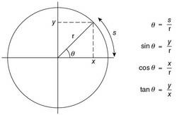
In addition to the seven base units of measurement (appendix A), there is a supplementary unit for measuring angle, the radian (rad). An angle (θ) is
equal to 1 rad (~57.3°) when the ratio of an arc length (s) to the radius of a circle (r) has a value of 1 (figure 1.1). As the ratio of two lengths, the radian is a dimensionless quantity. To become familiar with measuring angles in radians, recognize that a right angle is equal to 1.57 rad, the elbow joint is at an angle of 3.14 rad when the arm is extended, and one complete circle is 2π rad.
Figure 1.1 Definition of a radian.
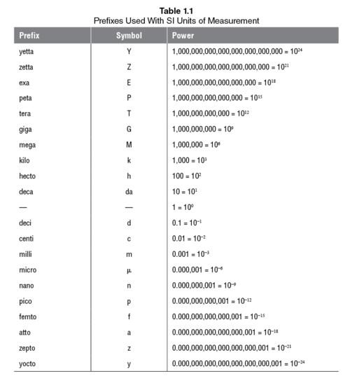
Because it is convenient for numbers to range from 0.1 to 9999, prefixes (table 1.1) can be attached to the units of measurement to represent a smaller or larger amount of the unit. The marathon (26 miles, 385 yd), for example, should be expressed as 42.4 km rather than 42,400 m; the prefix kilo (k) represents 1000, and 1 km = 1000 m. Similarly, prefixes can be used for small distances. For example, the diameter of a muscle fiber is most appropriately expressed in micrometers (μm; 1 μm = 0.000,001 m), with a typical value of 55 μm.
Changing Units
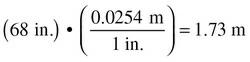
Sometimes it is necessary to change the unit of measurement from another system (e.g., English units) to an SI unit. Appendix A lists the SI units and some common conversion factors. To convert a quantity from one measurement system to another, write the required expression and cancel the units to produce the intended unit of measurement. For example, to convert your height (say 5 ft 8 in.) to SI units, multiply your height (68 in.) by the relation between inches and meters:
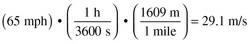
Similarly, to convert a speed from miles per hour (mph) to meters per second (m/s), convert hours to seconds and miles to meters by multiplying with the appropriate conversion factors as follows:
The advantage of using these procedures is that you will be less likely to invert a conversion factor if you pay attention to canceling units. If you are not familiar with SI units, then it is helpful to build familiarity by remembering reference values, such as your height (m), mass (kg), and weight (N), rather than memorizing conversion factors. Similarly, to judge whether or not a movement is fast, compare the speed of the movement with the average speed (10 m/s) of a person who runs 100 m in 10 s.
When converting units of measurement for area, the conversion factor must be squared. To convert centimeters squared to meters squared, for example, visualize a square with sides of 1 m (100 cm) in length and hence an area of 100 × 100 cm2 or 1 × 1 m2 . Thus, the area of the square is 10,000 cm2 or 1 m2; that is, 1 m2 = 1002 cm2 . Similarly, the conversion factor must be raised to a power of three when converting units of measurement for volume.
Accuracy and Significant Digits
When we measure a physical property of an object, we obtain an estimate of its true value. The closeness of the estimate to the true value indicates the accuracy of the measurement. The accuracy depends on the resolution of the measurement device. For example, if we measure the body mass of an individual who has an actual mass of 79.25 kg, we need a scale that can measure one-hundredths of a kilogram to obtain an accurate estimate. The digits in a number that indicate the accuracy of a measurement are known as the significant digits. The number 79.25 has four significant digits; the number 79.3 has three significant digits; and the numbers 79, 790, 7900,
0.79, and 0.079 all have two significant digits. When reporting data, one way to decide how many significant digits to use is to round the standard deviation to two significant digits and then match the mean to the number of decimal places in the standard deviation (Hopkins et al., 2009).
Two practices concerning significant digits are usually followed when performing calculations. First, the number of digits to the right of the decimal point in the answer when adding or subtracting should be the same as for the term in the calculation with the least number of significant digits to the right of the decimal point. Similarly, the answer when multiplying or dividing should have the same number of significant digits as the least accurate term in the calculation. Second, greater accuracy is required when estimating the difference to three significant digits when the measurements involve small differences. For example, if one group of subjects took 1.2503 s to perform a movement and another group took 1.2391 s, then the difference between the two groups would be 0.0112 s. To find the difference to three significant digits (0.0112), it was necessary to measure movement time to five significant digits.
Motion Descriptors
Movement involves the shift from one position to another. It can be described in terms of the size of the shift (displacement) and the rate at which it occurs (velocity and acceleration).
The position of an object refers to its location in space relative to a reference location. For example, the 100 m race in track and field refers to the position of the finish line relative to the start position; the height of a person specifies the position of the feet below the head; the width of a soccer goal indicates the position of one side of the goal relative to the other side; the third and fifth positions in ballet refer to the position of one foot with respect to the other; and so on. When an object experiences a change in position, it has been displaced and motion has occurred. Motion can be detected only by comparing an object’s position at one instant in time with its position at another instant. Motion, therefore, is an event that occurs in space and time.
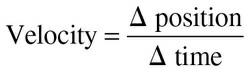
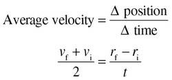
The term displacement indicates the size of the change in position, whereas the terms velocity and speed describe both the spatial (space) and temporal (time) aspects of the motion. Velocity tells us how fast and in what direction, whereas speed defines how fast. Because it has both magnitude and direction, velocity is a vector quantity that defines the change in position with respect to time. It indicates how rapidly the change in position occurred and the direction in which it took place. Speed is simply the magnitude of the velocity vector and does not indicate the direction of the displacement. Because displacement refers to a change in position, velocity can be described as the time rate (derivative) of displacement. In calculus terminology, velocity is the derivative of position with respect to time.
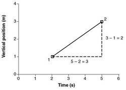
Figure 1.2 shows the vertical position of an object above some baseline value at two different instants in time. The figure indicates that the object was displaced by 2 m during the 3 s period and experienced an average velocity in moving from position 1 to position 2 of 0.67 m/s, where m/s refers to meters per second (this unit of measurement can also be expressed as m•s 1). Stated more explicitly,
where Δ (delta) indicates the change in each variable. Graphically, velocity refers to the slope of the position–time graph. Because a line graph (such as figure 1.2) shows the relation between two variables, a change in the slope of the line as it becomes more or less steep indicates a change in the relation between the variables. We determine the slope of the line numerically by subtracting an initial-position value from the final position (Δ position) and dividing the change in position (displacement) by the amount of time it took for the change to occur (Δ time). Slope, therefore, refers to the rate of change in a variable: The steeper the slope, the greater the rate of change; conversely, the lesser the slope, the slower the rate of change.
(1.1)
Figure 1.2 A position–time graph.
Many concepts in this text are presented in the form of graphs to show the relation between selected variables. Figure 1.2 shows the relation between position and time. The relation can be indicated as the line, or data points, plotted on the graph. The main purpose of a graph is to show the trend or pattern of the relation between the variables; more precise quantitative data are presented as tables or sets of numerical values. To interpret a graph, first identify the variables indicated on the axes and then examine the relation between the variables. The relation between position and time in figure 1.2 is relatively straightforward and can be represented by a single measurement, the slope of the line.
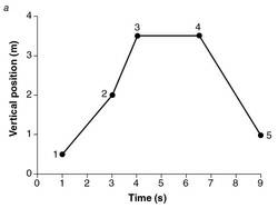
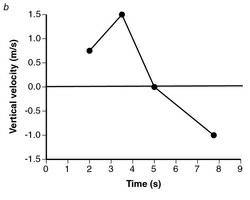
The displacement of an object can vary in both magnitude and direction. Figure 1.3a shows the vertical position of an object at five instances in time. The average velocity for each displacement can be calculated with equation 1.1: position 1 to 2 = 0.75 m/s; position 2 to 3 = 1.5 m/s; position 3 to 4 = 0 m/s; and position 4 to 5 = 1.0 m/s. These values are plotted in figure 1.3b. Velocity increases with the steepness of the slope of the position–time graph (figure 1.3a); for example, position 2 to 3 = 1.5 m/s versus position 1 to 2 = 0.75 m/s. A change in the direction of displacement is indicated by a difference in the slope of the line between two positions. The downward slope from position 4 to position 5 shows a downward vertical displacement and is indicated as a negative velocity in figure 1.3b. Conversely, the absence of a change in position (e.g., position 3 to 4) corresponds to a zero velocity. This example illustrates an important point about velocity: When the sign of the velocity value (positive, negative, or zero) changes, the movement has changed direction. Furthermore, when the direction of a movement changes, the velocity–time graph must pass through zero. Figure 1.3b indicates that an
object initially moved in one direction (arbitrarily called the positive direction note the positive slope in figure 1.3a), then was stationary (zero velocity), and finally moved in the other direction (negative slope).
Figure 1.3 (a) The variation in velocity associated with unequal changes in magnitude and direction in a position–time graph, and (b) the average velocities of the displacements.
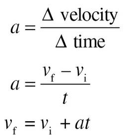
It is not sufficient to describe motion only in terms of displacement and velocity. For example, velocity is not constant when a ball held 1.23 m above the ground is dropped and reaches the ground 0.5 s later. The change in position is 1.23 m, and the average velocity is 2.46 m/s (1.23 m/0.5 s). But velocity changes over time. It begins with a zero velocity at release and increases to a value of 4.91 m/s just before contact with the ground after falling 1.23 m. The rate of change in velocity is referred to as acceleration; that is, acceleration is the derivative of velocity with respect to time or the second derivative of position with respect to time. The acceleration the ball experiences while it falls is constant and has a value of 9.81 m/s2; thus, acceleration indicates the change in meters per second each second (m/s2). Consequently,
(1.2)
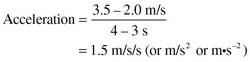
If the variable on the y-axis of figure 1.3a were changed to vertical velocity so that point 2 had the coordinates of 2.0 m/s and 3 s and point 3 had the coordinates of 3.5 m/s and 4 s, the rate of change from point 2 to point 3 (the acceleration) could be calculated with equation 1.2 as follows:
Similarly, the average acceleration for the other changes in vertical velocity would be as follows: point 1 to 2 = 0.75 m/s2; point 3 to 4 = 0 m/s2; and point 4 to 5 = 0.83 m/s2 . As with velocity, therefore, acceleration can have both magnitude and direction and thus is a vector quantity. Moreover, just as velocity can be represented graphically as the slope of the position–time graph, acceleration corresponds to the slope of the velocity–time graph.
The acceleration the ball experienced when it was dropped from a height of 1.23 m was due to the gravitational attraction between two masses planet Earth and the ball. The force of gravity produces a constant acceleration of approximately 9.81 m/s2 at sea level; this is usually written as 9.81 m/s2 to indicate the downward direction. A constant force always produces a constant acceleration; conversely, the absence of a force or the application of a pair of balanced forces means that the object is at rest or traveling at a constant velocity and does not accelerate.
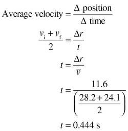
Example 1.1 Kinematics of the 100 m Sprint
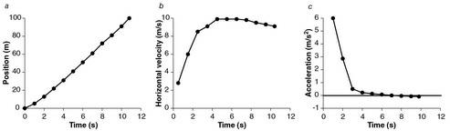
As an example of the relations among position, velocity, and acceleration, consider the kinematics of a person sprinting 100 m as fast as possible. To describe the kinematics of the performance we need to determine the position of the runner at various times during
the race. One way to do this is to record a video of the runner and measure the displacement of the hip joint. Figure 1.4a shows the position of the runner’s hip joint every 1 s, beginning the moment the race began and ending at 10.8 s when the runner crossed the finish line. The change in position between any two consecutive data points in figure 1.4a represents the displacement that occurred during that interval. The data in figure 1.4a show the position–time relation of the runner’s hip joint during the 100 m sprint.
From figure 1.3a, we know that the slope of the position–time graph tells us about the velocity of the runner. Because the runner moved toward the finish line during the entire sprint, velocity did not change direction and remained positive throughout the sprint. With the application of equation 1.1 to each interval of displacement, we can determine the average velocity for each interval and graph the velocity–time data for the runner as in figure 1.4b. Although we know that the runner began with a velocity of 0 m/s, the average velocity for the first interval (0-1 s) of available data was 2.8 m/s, which is plotted at the midpoint of the first interval. Similarly, we can derive the acceleration–time graph for the runner with equation 1.2 for each velocity interval and graph the data in figure 1.4c. Each acceleration value is plotted at the midpoint of the corresponding velocity interval. The positive and negative values in figure 1.4c indicate that the direction of acceleration was first positive (forward) and then slightly negative (backward).
Figure 1.4 (a) Position, (b) velocity, and (c) acceleration of a runner’s hip joint during a 100 m sprint.
Constant Acceleration
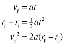
When acceleration is constant, motion can be described with some simple equations. These equations can be used to find the velocity of an object or the distance it has moved after it has been accelerated. From the elementary definitions of velocity (equation 1.1) and acceleration (equation 1.2), we can derive algebraic expressions involving time (t), position (r), velocity (v), and acceleration (a). In these equations of motion, the subscripts i and f indicate the initial and final values at the beginning and end of selected time (t) intervals, and the average (ā) and instantaneous (a) values for acceleration are the same because acceleration is constant. The resulting equations are as follows:
(1.3)
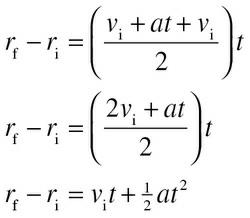
As described previously, a ball dropped from a height of 1.23 m will reach the ground 0.5 s later with a final velocity of 4.9 m/s. According to equation 1.3, the variables that influence final velocity are the initial velocity (v i) of the ball, the ball’s acceleration (a), and the duration of the fall (t). In this example, v i is 0, a is the acceleration due to gravity ( 9.81 m/s2), and t is 0.5 s. We can use a similar approach to determine how far an object will be displaced (Δr) after a given amount of constant acceleration. The equation is derived from our definition of velocity:
Substitute equation 1.3 for v f:
(1.4)
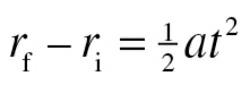
This equation indicates that the change in position (displacement) of an object depends on three variables: its initial velocity (v i), the constant acceleration (a) it experiences, and time (t). This relation can be used to determine the change in position of an object during a movement. As an example, consider an individual who dives off a 10 m tower. By varying the value of t from 0 to 1.5 s in 0.1 s increments, we can determine the change in position (r f r i) for each 0.1 s interval and thereby obtain the trajectory (position–time graph) of the diver during the performance. When the initial velocity of the diver is zero, as in this example, equation 1.4 reduces to
If we assume that the effects of air resistance are small and can be ignored, then the acceleration is simply that due to gravity and is constant during the dive. We can use equation 1.4 to determine the displacement during each 0.1 s interval and calculate the set of position–time data that represent the trajectory of the diver.
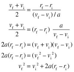
A similar approach can be used to derive an equation for determining the final velocity for an action as a function of displacement (equation 1.5) rather than time (equation 1.4).
In this expression t is unknown, so we rearrange equation 1.4 to express t as the dependent variable [t = (v f v i)/a] and substitute for t.
(1.5)
When the initial velocity for an interval is zero, such as for the object beginning at rest, then the equations can be simplified:
Example 1.2 Penalty Kick in Soccer
When a player takes a penalty kick in soccer, the goalie stands
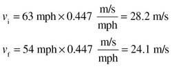
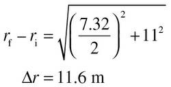
stationary in the middle of the goal (7.32 m wide) with the ball placed on the penalty spot (11 m in front of the goal). Suppose that a player made a penalty kick such that the ball left her foot with an initial velocity of 63 mph and traveled along the ground into the goal just inside the goalpost with a final velocity of 54 mph.
a. What was the velocity of the ball in SI units just after it left her foot and when it entered the goal?
b. What was the distance (change in position) the ball traveled from the penalty spot to the goal?
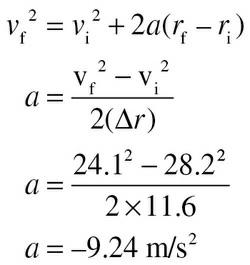
c. What was the average acceleration of the ball between the foot and the goal?
d. How much time did the goalie have to reach the ball from the moment it left the player’s foot until it entered the goal?
Example 1.3 Calculation of Velocity and Acceleration
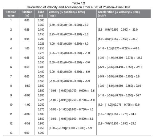
Kinematic analyses are usually based on a set of position–time data that are obtained with a motion capture system such as a video camera. A video record of a movement provides a set of still images (frames) that are subsequently projected individually onto a measuring device, and the locations of selected landmarks are determined. The positions of the landmarks are often expressed in x-y coordinates. Once we have a set of position–time data, we can use equations 1.1 and 1.2 to determine the average velocity and average acceleration between each position measurement. Table 1.2 provides an example of this procedure.
The 13 position values listed in table 1.2 indicate the location of an object at 13 different instants in time. The measurements show that the object first rose above an initial position (0.0 m) to a height of 1.0 m before being displaced by an equal amount ( 1.0 m) below the original position and finally returning to 0.0 m. We calculate the velocity of the object during this motion by applying equation 1.1 to the intervals of time for which position information is available.
Table 1.2 shows velocity as determined for each interval between two measurements of position. The first velocity value, for example, was obtained by dividing the displacement during the first interval (0.59 0.0 = 0.59 m) by the time elapsed during the interval (0.1 0.0 = 0.1 s) to yield the velocity for that interval (0.59/0.1 = 5.9 m/s). The calculated value (5.9 m/s) represents the average velocity over that interval and consequently is recorded in table 1.2 at the midpoint in
time of the interval (0.05 s). Similarly, the first acceleration value ( 23.0 m/s2), which was determined with equation 1.2, is listed at the midpoint in time (0.10 s) of the first velocity interval (0.05-0.15 s).
By this procedure the average value of velocity is determined for each position interval and the average acceleration is calculated for each velocity interval. Thus, from a set of 13 position measurements, we calculate 12 values for velocity and 11 for acceleration.
The data in table 1.2 indicate that velocity is positive when position increases (positions 1 to 4 and 10 to 13) and is negative when position decreases (positions 4 to 10). A similar relation exists between the slope (increase or decrease) of the change in velocity and the sign of the acceleration values. These relations among position, velocity, and acceleration are shown in figure 1.5.