INTRODUCTION TO CEM SYSTEMS
In the early 1970s, a better way was needed to monitor stack emissions than by manual stack tests. In general, manual methods are conducted by inserting a probe into a stack, extracting a sample, and analyzing the sample in a laboratory, which is a time-consuming process. Manual source tests also require a degree of preparation, and the coordination and prior scheduling of a test may result in source operations being highly tuned before such testing takes place. Manual test results, therefore, may not necessarily be representative of day-to-day emissions. Clearly, for monitoring plant emissions and the performance of pollution control equipment on a more realistic basis, alternative measurement techniques are needed.
A BRIEF HISTORY
Attempts were made in the 1960s to use ambient air analyzers and process industry analyzers to measure source emissions. Ambient air analyzers were not successful at that time due to the instability of dilution systems. However, process analyzers did prove to be useful, particularly those that employed ultraviolet and infrared photometric techniques. Then, in the late 1960s and early 1970s, successful developments emerged in instrumentation in Germany and the United States. Ambient analyzers were redesigned to measure gases at higher concentration levels, and the so-called “in-situ” analyzers were developed, which can measure gases in the stack without sample extraction. These methods, in addition to new German optical systems for opacity monitors and the development of luminescence measurement techniques in
the United States, provided a technological base from which continuous emission monitoring (CEM) regulations could be established.
Continuous emission monitoring requirements in the United States were first promulgated in 1971. However, the CEM industry did not begin to develop until after 6 October 1975 when the U.S. Environmental Protection Agency (U.S. EPA) established performance specifications for CEM systems and required their installation in a limited number of sources. Since then, CEM systems have been applied to a wider range of sources, and over 50 years of experience has led to the evolution of analyzers and monitoring systems with ever-improving performance The technology is considered mature, having a solid foundation in reliable instrumentation, procedures, and standards that can assure the quality of source emission data at specified limits of accuracy and precision.
The earliest focus of CEM technology was on the analyzer – the instrument that measures. However, it was soon found that the process of transporting the gas to the analyzer was a source of many problems. Such problems were addressed in a number of ways by CEM “systems” integrators. Those who understood the effects of corrosive stack gases on materials and the effects of pressure and temperature on gas transport were the first to design and successfully market systems that worked under severe sampling conditions.
The difficulties associated with extractive systems led to the idea of measuring the flue gases as they exist in the stack or duct, without conditioning. This idea was realized in the development of “in-situ” analyzers, secondgeneration source monitoring systems especially designed
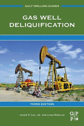
to avoid problems inherent in extracting gases. In-situ systems have been designed to measure gas concentrations, flue gas opacity, flue gas flow, and particulate matter concentrations. Many present-day CEM systems are a combination of extractive and in-situ systems (Figure 1-1).
Third-generation systems emerged with the promulgation of the Clean Air Act Amendments of 1990 and the implementation of the acid rain allowance trading program. Requirements to report emissions in tons per year led to the demand for systems that could measure pollutant mass rate. As a result of this program, flow monitors and dilution-extractive systems were added to the inventory of monitoring methods. It was in the acid rain program that CEM systems found their maturity. To assure the success of plant monitoring programs, both equipment and personnel resources were made available by corporate management. And here, it was found that for the success of monitoring programs, trained and experienced personnel can be equally important as the equipment.
A fourth wave of continuous emission monitoring applications came after 2000 with the delayed and piecemeal regulatory development of rules for hazardous air pollutants. The program to control hazardous air pollutant emissions was promulgated in the 1990 Clean Air Act Amendments along with the acid rain program; however, due to the enormity of the task of regulating 187 hazardous air pollutants from 174 source categories, the program was slow to start. It wasn’t until after 2000 that
continuous monitoring requirements for air toxics began to come into effect, but the need to develop new and more sophisticated monitoring systems for measuring particulate matter, mercury, and hydrochloric acid was apparent before that time. A new generation of monitoring systems was developed, measuring a wider range of compounds and materials, at ever lower concentrations, by incorporating advanced measurement and miniaturization techniques developed in response to national military and security concerns.
The business of continuous emission monitoring is largely dependent upon environmental regulations and is almost cyclical with the ebb and flow of environmental rule-making. As new regulatory programs are developed, it is found necessary that a means be provided to keep track of progress or lack of progress. When emission limits are mandated, enforcement programs require a measure of whether emission limits are met or not. Intermittent manual stack testing is clearly not adequate for this purpose, and it has been demonstrated that continuous emission monitoring systems can provide data of sufficient precision and accuracy to support enforcement programs and allowance trading programs. With emission limits becoming ever more stringent and the proper operation of pollution control equipment ever more critical, continuous emission monitoring systems have evolved where they can today, meet the most demanding applications.
TYPES OF MONITORING SYSTEMS
A CEM system is actually composed of several subsystems: the sampling interface, the gas analyzer(s), and the data acquisition/controller system. The sampling interface is a subsystem that either transports or separates the flue gas from the analyzer. CEM systems are characterized in terms of the design of this interface. In extractive systems, the interface consists of a system that extracts and conditions the gas before entering the analyzer. In in-situ systems, the interface is simpler, composed of flanges designed to align or support the monitor and blower systems used to minimize interference from particulate matter. The data acquisition/controller subsystem is integral to the proper operation of the total system. The control system controls automatic functions of the system, such as calibration, probe purging, and alarming. The data acquisition system receives the analyzer data, converts it into appropriate units, records it, and provides reports for both internal and external use. Today, CEM data acquisition systems are frequently networked to engineering, corporate, and even agency offices, where the data are used for a variety of operational and management purposes. Both extractive and in-situ systems operate in the source environment and must operate continually under changing stack and ambient conditions. Although this is not necessarily a problem for properly designed and maintained systems, alternative approaches have been sought. One of these approaches, remote sensing, has been applied with limited success, but has not been used widely. Another alternative, the correlation of stack emissions to process parameter data, has led to computerized “predictive emission monitoring systems” or PEMS. These systems have been employed successfully in a number of applications and have considerable potential if used in tandem with extractive or in-situ monitoring
hardware. The monitoring methods discussed earlier are classified in Figure 1-2 and discussed further in the following sections.
Extractive Systems
Extractive gas monitoring systems were the first to be developed for source measurements. In these systems, gas is extracted from a duct or stack and transported to analyzers to measure the pollutant concentrations. Many of the early extractive systems first diluted the gas using rotameters, and then applied ambient air analyzers for measurements. However, frequent problems occurred in maintaining stable dilution ratios, so analyzers were subsequently developed to directly measure the flue gas at source-level concentrations in the range of 100–1000 ppm or higher. These source-level extractive systems were quite successful and received their widest application in the 1970s and early 1980s.
Many of the problems associated with the earlier dilution systems have since been eliminated by new techniques developed in the 1980s. The advent of the “dilution probe” made dilution systems viable for source measurements. Dilution systems are now relatively easy to construct and exhibit good performance. They are particularly useful for monitoring water-soluble gases and provide a platform for the application of a new generation of analyzers that are able to measure part per billion concentration levels.
In order for an instrument to measure gas concentrations, the gas sample must be free of particulate matter. Often, water vapor is removed and the sample is cooled to instrument temperature. This requires the use of valves, pumps, chillers, sample tubing, and other components necessary for gas transport and conditioning. “Hotwet” systems, which measure hot gases without water
removal, operate continuously at elevated temperatures, eliminating the need for water removal systems. Extractive systems use an umbilical line to transport the flue gas sample from the stack or duct to an analyzer cabinet or temperature-controlled shelter. This line is heated in source-level systems where the conditioning system is located in the shelter.
Dilution-extractive systems became popular in the 1990s for determining pollutant mass emission rates at U.S. coal-fired power plants subject to acid rain cap-andtrade regulations. Dilution-extractive CEM systems measure on a wet basis, an advantage when required to report emissions in units of tons/year or kg/hr. Dilutionextractive systems are available where the sample dilution takes place in a specially designed in-stack probe or, alternatively, in a probe box outside of the stack, where a variety of dilution techniques are available. In either case, when the flue gas sample is diluted at the stack, a heated umbilical line is not always needed to transport the diluted sample to a CEM shelter.
Close-coupled systems are extractive systems where the sample conditioning and analysis are conducted directly on the stack. In these systems, the analyzer is connected directly to the sample probe. These systems avoid sample losses for “sticky” or reactive gases due to gas transport and also reduce system costs by not requiring an umbilical line.
In-Situ Systems
In-situ systems consist primarily of an analyzer that employs some type of sensor to measure the gas directly in the stack, or projects light through the stack to make measurements. The opacity monitor and flow monitor illustrated in Figure 1-1 are typical examples of in-situ analyzers. There are two classifications of in-situ analyzers: point and path. Point analyzers consist of an electrooptical or electroanalytical sensor mounted on the end of a probe that is inserted into the stack. The point instack measurement is usually made by a sensor over a distance of only a few centimeters. Path analyzers, on the other hand, measure along a path across the width of the duct or diameter of the stack. In these “cross-stack” gas analyzers, light is transmitted through the gas, and the interaction of the light with the flue gas is used to obtain a quantitative value of the pollutant concentrations. In single-pass instruments, light is transmitted from a unit on one side of the stack to a detector on the other side, making only one pass through the stack. In a double-pass system, light is reflected from a mirror on the opposite side, doubles back on itself, and is detected back at the “transceiver.”
In-situ analyzers are used to measure the concentrations of pollutant and combustion gases and particulate matter, flue gas opacity, and flue gas velocity (flow). Both
point and path techniques are used to monitor gas and particulate concentrations. Opacity monitors (transmissometers) are path monitors and can be either singlepass or double-pass systems, measuring the transmittance of visible light through the stack. Flow monitors are designed in either point or path configurations, depending upon the analytical technique.
Using wavelength-tunable lasers, in-situ gas monitoring systems are experiencing renewed popularity, particularly for the measurement of reactive gases such as HCl and NH3. More attention is being paid to verifying system calibration using NIST traceable calibration gases, an important issue in the United States. In-situ point monitors using laser-light scattering techniques have become popular for monitoring flue gas particulate matter concentrations. Light-scattering particle sizing techniques are developing, but this technology has lagged behind in source monitoring applications for many years.
Remote Sensors
Remote sensing systems have no interface between the stack gases and the sensing instrument, other than the ambient atmosphere. They thus avoid problems associated with a stack or duct interface. These systems can detect emission concentrations merely by projecting light up to the stack (active systems) or by sensing the light radiating from the “hot” molecules emitted from the stack (passive systems). However, due to an inherent problem in defining the length of the measurement path in the plume, the accuracy of gas concentration data is poorer than that obtained by the extractive or in-situ techniques. This problem is also an issue in making flue gas measurements using laser systems mounted on unmanned aerial vehicles (drones), a developing source monitoring technology.
The U.S. EPA has developed Method 9A for monitoring stack exit opacity, using a laser light detection and ranging technique (LIDAR). The method is particularly useful at night or under atmospheric conditions that are not favorable to a visible emissions observer (VEO) performing EPA test method 9. In a related development, a digital camera technique for measuring plume opacity has been standardized by ASTM in ASTM standard D7520-16. Although not a continuous method, data using this method are being accepted by regulatory agencies for visible emissions compliance determinations.
Test methods and certification procedures have not been standardized for remote sensing systems used to monitor gaseous emissions. Since the regulatory applicability of remote pollutant gas measurements to stationary sources has not yet been established, these systems for source emissions monitoring are not extensively applied in commercial applications. They have, however, seen wider application in “fence-line” monitoring,
particularly at petroleum refineries and chemical plants. Attempts are frequently made to correlate emissions data with long-path remote sensing data obtained along a plant perimeter. Such correlations typically devolve into research studies and have met with limited success as a regulatory tool.
Unmanned aerial vehicles (UAVs) (drones) offer significant potential in source monitoring applications (Villa et al. 2016). UAV systems can obtain grab sample for laboratory analysis, or, as part of an active remote system, incorporate a stationary mirror to reflect light projected from a ground-based analyzer. Using lasers, two drones standing-off from a stack exit can make crossstack gas measurements. Four drones could measure on two diameters. UAV platforms can carry simple miniature sensors, readily available from hand-held monitors, to measure flue gases in real time using a stand-off probe or by flying through the stack. For compliance measurements, a probe can be inserted from the UAV “down” the stack, as it hovers at a fixed position next to the stack. The availability, at present, of miniature and micro analyzers provides many options for analysis using UAV platforms. Flares and smaller process stacks with limited access or without sampling platforms are seen as potential applications for this technology.
Performance specification and certification procedures have not been developed for remote sensing systems or UAVs; however, this technology is relatively new. Calibration procedures and precision and accuracy issues relative to in-stack measurements must first be standardized for UAV data to be credible. Standards developed by independent standards bodies such as ASTM or ISO may provide a basis for future agency requirements. Because the regulatory applicability of remote and UAV pollutant gas measurements to stationary sources has not yet been established, they will not be discussed further, but do bear watching in the technical literature.
Parameter Monitoring Systems
Alternative approaches to emissions monitoring have been developed that do not require the use of analytical instrumentation, but rely instead on inputs from process sensors, such as thermocouples, pressure transducers, and fuel flow meters. Data from these sensors can be used in a variety of ways in environmental regulatory programs. The parameter information can be either used directly as a surrogate to substitute for concentrationbased emissions data or it can be incorporated into a model to predict emissions.
U.S. regulatory programs have long used parameter data such as pressure drop or temperature to monitor the performance of emission control equipment. The parameter data has been used either as a regulatory trigger to initiate enforcement action directly or as an indicator of
noncompliance with permit conditions. Control equipment and unit operational parameters can also be used directly in continuous parameter monitoring systems (CPMS) as part of a continuous monitoring system (CMS). This regulatory approach does not require the use of continuous emission monitoring systems although a CEM system can be a part of a CMS. The U.S. air toxics standards make extensive use of this method.
A more recent approach has been used to develop emission models based on process parameter data. Models are developed by first correlating parameter data to emissions data. An initial study is performed by varying and monitoring process and control equipment parameters while monitoring flue gas emissions using reference methods or CEM systems. One can then correlate the data using engineering calculations, least squares methods, or neural net techniques to develop a model that “predicts” emissions from parameter data. Such predictive emission monitoring systems (PEMS) employ from 3 to 20 input parameters and have been applied to a variety of sources. They are most successful on sources with minimal variation in fuels and operating conditions.
Analytical Techniques Used in CEM System Instrumentation
The analytical techniques used in extractive and in-situ CEM systems encompass a wide range of chemical and physical methods. These vary from chemical methods using simple electrochemical cells to advanced electrooptical techniques such as wavelength modulation and Fourier-transform infrared spectroscopy. Table 1-1 summarizes the analytical techniques that are used in currently marketed CEM systems for gases. Table 1-2 gives a summary of analytical techniques used in continuous emission monitoring systems for particulate matter (PM CEMS).
Techniques used for laboratory analysis, as well as techniques applied specifically for emissions monitoring, have been incorporated into commercially marketed systems. New analyzers have been developed using established electro-optical methods, but are beginning to incorporate new light sources and detectors, such as tunable diode lasers, quantum cascade lasers, and diode arrays and new techniques such as cavity ringdown spectroscopy. The incorporation of microprocessors into today’s analyzers has added useful features such as data storage, troubleshooting diagnostics, and external communication.
To lower the cost of CEM systems, CEM system manufacturers are employing multi-gas techniques to avoid subsystem duplication that occurs when using single-gas dedicated analyzers. One approach is to use multi-gas methods such as dispersive, FTIR, or photoacoustic
TABLE 1-1 Analytical Techniques Used in Continuous Emission Monitoring Systems for Gases and Volumetric Flow/Velocity Gases
Flow/Velocity
Extractive In-situ In-situ
Absorption spectroscopy:
Differential absorption
Photoacoustic
Gas filter correlation
Fourier transform IR
Luminescence methods:
Fluorescence (SO2)
Chemiluminescence (NOx)
Electroanalytical methods:
Polarography
Potentiometry
Calorimetry
Electrocatalysis (O2)
Paramagnetism (O2)
Methods for HAPS:
Differential absorption
Gas chromatography
Mass spectrometry
Fourier-transform IR
Ion-mobility spectrometry
Atomic emission (Metals)
Atomic absorption (Metals)
Atomic fluorescence (Metals)
Path:
Differential absorption – IR/UV
Second-derivative spectroscopy
Wavelength modulation
Gas filter correlation
Point:
Differential absorption – IR/UV
Gas filter correlation
Path:
Acoustic velocimetry
Time-of-flight
Point:
Differential pressure
Thermal sensing
TABLE 1-2 Analytical Techniques Used in Particulate Matter Continuous Emission Monitoring Systems (PM CEMS)
Extractive In-Situ
Point Point:
Beta radiation attenuation
Light scattering
Light scattering
Contact charge transfer
Electrodynamic induction
spectrometry. Another approach is to incorporate discrete, multiple, and interchangeable sensors into a single chassis.
Succeeding chapters present details of both extractive and in-situ systems – their advantages, disadvantages, and limits of application. The sampling interface is of particular importance in extractive system design and is treated separately in Chapter 3. Extractive system analyzers are discussed in Chapter 5. For in-situ system design, the analyzer type is most important. In-situ monitors for measuring gases are discussed in Chapter 6 and monitors designed for measuring flue gas flow, opacity and particulate matter in Chapters 7–9.
Mercury monitoring, a field in itself, has advanced significantly, within 15 years of research and development.
Path
Transmissometry
Light scattering
This topic is treated separately in Chapter 12, to outline how a new generation of mercury monitoring systems has evolved to enable continuous monitoring of stationary source mercury emissions down to less than 1 μg/m3. Monitoring for hazardous air pollutants (HAPs) has developed along with increased concerns over their toxic effects. Monitoring requirements for these materials, implemented incrementally over the past 20 years, are discussed in Chapter 13.
Data Acquisition and Handling Systems
CEM system analyzers do not stand alone, but are part of a larger system as seen in Figure 1-1. The assembly of
analyzers is coordinated and controlled to provide emissions data that are subsequently recorded and reported. These roles were all originally considered part of the data acquisition and handling system (DAHS or DAS). Today, control functions are commonly separated from the DAHS by using data loggers, programmable logic controllers (PLCs), or separate microprocessor systems. This simplifies the CEM system by providing more flexibility for both system control and data acquisition and reporting.
Hardware used in CEM recording and reporting systems has evolved from the now archaic strip chart recorders to computer systems integrated into the plant distributive control system and the plant local area network, corporate wide area network, or intranet. In special cases, remote terminal units are used to provide emissions data to environmental control agencies either continuously on a real-time basis or on demand.
CEM software has evolved significantly, principally due to the demands of the U.S. EPA Acid Rain Program. Requirements to report all emissions data plus plant operational data, on a quarterly basis, have led to sophisticated multitasking programs, having the capability of editing and back-filling data according to prescribed algorithms. Today’s programs offer flexibility to both CEM system operators and environmental engineers in evaluating data quality and in preparing internal and external reports.
Programming tends to be customized to meet the demand of each plant installation with flexible and userconfigurable programs, making this task somewhat easier. The integration of CEM system data into plant distributive control systems and information networks has become a larger task. This requires considerable coordination between plant information technology personnel, plant engineers, the CEM system integrator, and the data acquisition system provider. This is often the most difficult job associated with the installation of a new CEM system.
THE ROLE OF QUALITY ASSURANCE
In the 1970s, industry frequently presented quite valid arguments that the performance of continuous monitoring systems was questionable. Two basic principles of CEM technology were soon learned:
1. There is no one “best” type of system for all applications.
2. A CEM system must be maintained if it is to operate.
During this period, aggressive CEM system vendors frequently sold their systems to anyone who could be convinced to buy their product. This resulted in
misapplications of both in-situ and extractive systems. The resulting poor performance led to unfortunate perceptions about the reliability of the technology and bankruptcy and absorption of several companies. This is a process that continues still today. From this experience, formal procedures for specifying and evaluating CEM systems have been developed and should be used by companies planning major CEM system purchases.
Errors in application have not been the only reason for poor CEM system performance. It is often assumed that after a CEM system is installed, it can generate data as routinely as a thermocouple or pressure gauge. It must be realized that routine maintenance programs are necessary for the continuing operation of extractive system plumbing and electro-optical systems. Although this necessity is now well understood, awareness of this need did not develop in the United States until the early 1980s. A CEM specialty conference of the Air Pollution Control Association held in Denver in 1981 pointed out the need for established and effective CEM system quality assurance (QA) programs. By the time of a subsequent conference held in Baltimore in 1985, the U.S. Environmental Protection Agency proposed CEM system quality assurance requirements and many companies were reporting the success of their own QA programs in improving CEM system performance. In 1989, the U.S. EPA promulgated quality assurance procedures for CEM systems used for compliance determinations, specifying requirements for calibration and periodic audits. With this lesson learned, when new performance specifications are promulgated, quality assurance procedures specific to the pollutant are published concurrently. This can be seen in the almost concurrent publication of Appendix F quality assurance procedures for particulate monitoring systems, mercury monitoring systems, and hydrochloric acid monitoring systems with the publication of their respective performance specifications in Appendix B of Part 60.
Like an automobile, where the oil must be changed and the tires rotated, a CEM system requires routine checks and replacements. QA programs incorporating daily and weekly checks, periodic audits, and preventive maintenance procedures have been found to be the key to continuing CEM system operation. Systems with such programs today show better than 98% data availability.
APPLICATION
CEM systems were originally required by regulatory agencies in the United States for monitoring the effectiveness of air pollution control equipment in removing pollutants from flue gases. As indicators of control equipment performance, the data could be used to track plant performance and target sources that were not meeting their
emission limitations. Manual source tests would then be conducted on targeted sources to determine if, indeed, they were failing to be in compliance with emission limitations.
However, the extension of CEM data to direct enforcement applications has grown in both federal and state programs. By stating specifically in a rule or permit that a CEM system provides enforceable data that determines if an emission limit is being met or exceeded, the earlier link to control equipment performance is not as important. In addition, the promulgation of the “credible evidence” rule now allows the use of CEM system data in litigation.
CEM systems also provide the basis for the U.S. EPA acid rain control program mandated in the 1990 Clean Air Act Amendments. Here, CEM systems determine the “allowances,” the number of tons per year of SO2 emissions that are traded between the electrical utilities. This successful regulatory program has led to significant SO2 reductions in the United States within two years of its implementation. The over 2000 utility CEM systems installed to track allowances have contributed much to this success, providing an accurate database necessary to instill confidence in the trading market.
Another trading program is found in the Cross-State Air Pollution Rule, where NOx emissions are traded between electrical utilities and other sources in the northeastern states. These regulatory programs as well as economic forces led to an 89% decrease in SO2 emissions and an 82% decrease in NOx emissions from 1995 to 2017.
Although emission monitoring systems have been applied principally to satisfy such regulatory requirements, CEM system data can also be used proactively by plant and corporate management by providing a base of information on compliance status or for consideration in legal issues. As a result of both agency environmental programs and proactive source monitoring, the CEM database provides assurance to the public that emissions are being monitored to address environmental concerns.
However, the essential purpose of CEM systems should not be forgotten when providing for the timely submission of emissions reports. That purpose is to use CEM system data to control plant operations to meet emissions limitations (Figure 1-3). The continuous record of emissions data enables plant operators and engineers to optimize plant performance and control equipment operation. On a continuous basis, emissions can then be maintained within regulated limits. In some cases, operating costs can be reduced and data can be gathered for plant design and maintenance information. In sum, the focus should not be on the quarterly emissions report, but rather, on how to use the data to improve operational efficiencies to minimize emissions.
Plant emissions Continuous emissions data
Plant operations control
Emissions reporting
Figure 1-3 Industry uses of CEM system data.
SUMMARY
The technology of continuous emissions monitoring has not been static. The use of CEM systems for allowance trading programs and emissions enforcement programs, the demands for increased system availability, and advances in data handling and reporting have led to more sophisticated systems with better reliability. CEM systems have advanced considerably over 50 years of development, with improved sampling techniques, analyzers, and data processing systems being integrated into today’s systems to meet the challenges posed by new requirements. Also, by implementing CEM system quality assurance programs and by properly managing the monitoring programs, high system availability can be achieved. This high availability is a necessity today, where inaccurate data or missing data can incur both regulatory and economic penalties.
BIBLIOGRAPHY
Air Pollution Control Association (1981). Proceedings –Continuous Emission Monitoring: Design, Operation and Experience. SP-43. Pittsburgh: AWMA.
Air Pollution Control Association (1986). Transactions –Continuous Emission Monitoring – Advances and Issues. TR-7. Pittsburgh: APCA.
Air Pollution Control Association (1990). Proceedings –Continuous Emission Monitoring – Present and Future Applications. SP-71. Pittsburgh: AWMA.
Air Pollution Control Association (1993). Continuous Emission Monitoring – A Technology for the 90s. SP-85. Pittsburgh: AWMA.
Air Pollution Control Association (1995). Acid Rain & Electric Utilities – Permits, Allowances, Monitoring & Meteorology VIP-46. Pittsburgh: AWMA.
Air Pollution Control Association (1996). Continuous Compliance Monitoring Under the Clean Air Act Amendments. VIP-58. Pittsburgh: AWMA.
Air Pollution Control Association (1997). Acid Rain & Electric Utilities II. Pittsburgh: AWMA.
Baumbach, G. (1996). Air Quality Control: Formation and Sprces, Dispersion Characteristics and Impact of Air Pollutants - Measuring Methods. Techniques for Reduction
of Emissions and Regulations for Air Quality Control Springer. Berlin.
Baukal, C.F. (2011). Industrial Combustion Testing. Boca Raton: CFC Press.
Central Pollution Control Board (CPCP) (2018). Guidelines for Continuous Emission Monitoring Systems. Revision-01. Delhi, India. Central Pollution Control Board. http://www. indiaenvironmentportal.org.in (accessed 3 June 2021).
Cohn, P.E. (2006). Analisadores Industriais. Rio de Janeiro: Instituto Brasileiro de Petróleo e Gás. Editora Interciência Ltda.
Curtis, D., Averdieck, W., Kanchan, S.K., and Parre, A.A. (2018). CEMS: Continuous Emission Monitoring System: A Technical Guidance Manual. New Delhi: Centre for Science and Environment.
Down, R.D. and Lehr, J.H. (ed.) (2004). Environmental Instrumentation and Analysis Handbook. Wiley. Electric Power Research Institute (1993). Continuous Emissions Monitoring Guidelines: 1993 Update. Report No. EPRI TR-102386 V1 & V2. Palo Alto, CA: EPRI.
Environment Canada (2005). Protocols and Performance Specifications for Continuous Monitoring of Gaseous Emissions from Thermal Power Generation. EPS 1/PG/7. Ottawa: Environment Canada. European Commission (2017). Guidance Document. The Monitoring and Reporting Regulation – Continuous Emissions Monitoring Systems (CEMS). European Commission Directorate General Climate Action. https:// ec.europa.eu/clima/sites/clima/files/ets/monitoring/docs/ gd7_cems_en.pdf (accessed 3 June 2021)
Federal Ministry of the Environment, Nature Conservation and Nuclear Safety (2008). Air Pollution Prevention Manual on Emission Monitoring. Research Report 360 16 004 UBA – FB 001090. Dessau-Rosslau, Germany. Federal Environment Agency.
Indiana Department of Environmental Management (IDEM) (2017). Compliance Branch Guidance Manuals. CEMS/ COMS, Forms and Information and Guidance. Indiana Department of Environmental Management Office of Air Quality – Compliance. www.in.gov/idem/airquality (accessed 3 June 2021).
International Energy Agency (IEA) (1997). International Workshop on Continuous Emissions Monitoring. London: IEA Coal Research.
International Energy Agency (IEA) (1998). CEM98 –International Conference on Emissions Monitoring. EPA 450/2-84-004. London: IEA Coal Research.
Jahnke, J.A. (1984). Transmissometer Systems – Operation and Maintenance, an Advanced Course. EPA 450/2-84-004. Environmental Protection Agency-Air Pollution Training Institute. Research Triangle Park
Jahnke, J.A. (1991). APTI Course 474 – Continuous Emissions Monitoring Systems. EPA 450/2-91006A. Environmental Protection Agency-Air Pollution Training Institute. Research Triangle Park.
Jahnke, J.A. (1993). Continuous Emission Monitoring, 1ee. New York: Van Nostrand Reinhold.
Jahnke, J.A. (1994). An Operator’s Guide to Eliminating Bias in CEM Systems. EPA 430-R-94-016. Environmental Protection Agency-Acid Rain Division.
Jahnke, J.A. (2000). Continuous Emission Monitoring, 2ee. New York: Wiley.
Jahnke, J.A. and Aldina, G.J. (1979). Continuous Air Pollution Source Monitoring Systems Handbook. EPA 625/6-79-005. Cincinnati, OH: Environmental Protection Agency-Center for Environmental Research Information.
Jahnke, J.A., Peeler, J.W., Juneau, P.J., and Kinner, L.L. (1997). Handbook – Continuous Emission Monitoring Systems for Non-criteria Pollutants. EPA/625/R-97/001.
Jiang, Y., Yong, L., and Hongjie, L. (ed.) (2000). Stationary Source Emissions and Continuous Automatic Monitoring, Chinesee. China Standard Press.
Lillis, J.E. and Schueneman, J.J. (1975). Continuous emission monitoring: objectives and requirements. Journal of the Air Pollution Control Association 25 (8): 804–809.
Lipták, B.G. and Venczel, K. (2016a). Instrument and Automation Engineer’s Handbook – Fifth Edition Volume I Measurement and Safety. Boca Raton: CRC Press.
Lipták, B.G. and Venczel, K. (2016b). Instrument and Automation Engineer’s Handbook – Fifth Edition Volume II Analysis and Analyzers. Boca Raton: CRC Press.
New Jersey Department of Environmental Protection (2010). Guidelines for Continuous Emissions Monitoring System (CEMS), Continuous Opacity Monitoring Systems (), Periodic Monitoring Procedures (PMPS), and Annual Combustion Adjustments (ACAs). Technical Manual #1005. New Jersey Department of Environmental Protection – Air Quality Permitting Program Bureau of Technical Services. www.state.nj.us/dep/aqpp/techman.html (accessed 3 June 2021).
Pennsylvania Department of Environmental Protection (PADEP) (2006). Continuous Source Monitoring Manual –Revision 8. 274-030-001. Pennsylvania Department of Environmental Protection. www.dep.pa.gov (accessed 3 June 2021)
Rausch, A., Werhahn, O., Witzel, O., Ebert, V., Vuelban, J., Gersl, J., Kvernmo, G., Korsman, J., Coleman, M., Gardiner, T., and Robinson, R. (2015) Metrology to Underpin future Regulation of Industrial Emissions. 17th International congress of Metrology, 07008. 07008. www.cfmetrologie.edpsciences.org. (accessed 24 January 2022)
Schakenbach, J., Vollaro, R., and Forte, R. (2006). Fundamentals of successful monitoring, reporting and verification under a cap-and-trade program. Journal of the Air & Waste Management Association 56: 1576–1583.
Skoog, D.A., West, D.M. Holler, F.J., and Crouch, S.R. (2017). Principles of Instrumental Analysis, 7ee. Boston, MA: Cengage Learning.
U.S. EPA (2020a). Code of Federal Regulations – Standards of Performance for New Stationary Sources. 40 CFR 60. Washington, DC: Office of the Federal Register.
U.S. EPA (2020b). Code of Federal Regulations – Performance Specifications, 40 CFR 60 Appendix B. Washington, DC: Office of the Federal Register.
U.S. EPA (2020c). Code of Federal Regulations – Quality Assurance Procedures. Protection of the Environment, 40 CFR 60 Appendix F. Washington, DC: Office of the Federal Register.
U.S. EPA (2020d). Code of Federal Regulations – National Emission Standards for Hazardous Air Pollutants for Source
Categories, 40 CFR 63. Washington, DC: Office of the Federal Register
U.S. EPA (2020e). Code of Federal Regulations – Permits Regulation, 40 CFR 72. Washington, DC: Office of the Federal Register
U.S. EPA (2020f). Code of Federal Regulations – Sulfur Dioxide Allowance System. 40 CFR 73. Washington, DC: Office of the Federal Register.
U.S. EPA (2020g). Code of Federal Regulations – Continuous Emission Monitoring. 40 CFR 75. Washington, DC: Office of the Federal Register.
U.S. EPA. (2020h). Code of Federal Regulations – Specifications and Test Procedures, 40 CFR 75 Appendix A. Washington, DC: Office of the Federal Register.
U.S. EPA (2020i). Code of Federal Regulations – Quality Assurance and Quality Control Procedures, 40 CFR 75 Appendix B. Washington, DC: Office of the Federal Register. Vermont Air Quality and Climate Division (2002) Continuous Emission Monitoring Regulations – Revision 5. Vermont Department of Environmental Conservation. www.dec. vermont.gov (accessed 3 June 2021).
Villa, T.F., Gonzalez, F., Mljievic, B. et al. (2016). An overview of small unmanned aerial vehicles for air quality measurements: present applications and future perspectives. Sensors 16 (1072): 1–29.
Wenlong, W., Xiaofeng, T., Song, C. et al. (ed.) (2011). Thermal Power Plant Continuous Flue Gas Emission Monitoring System Technology and Use. Beijing, China: Electric Power Press.
White, J.R. (1995). Survey your options: continuous emissions monitoring. Environmental Engineering World July-August: 6–10.
Wiegleb, G., Franconia, O., Reinmann, J. et al. (2016). Gasmesstechnik in Theorie und Praxis . Springer Vieweg.
Willard, H.H., Merritt, L.L., Dean, J.A., and Settle, F.A. (2004). Instrumental Methods of Analysis, 7ee. New York: CBS Publishers.
Zhang, C. (2007). Fundamentals of Environmental Sampling and Analysis. Hoboken: Wiley.
CEM REGULATIONS
Environmental control agencies have been the driving force for the installation of continuous emission monitoring systems. The emergence of CEM regulation in the 1970s brought a new perspective to emissions monitoring by requiring a wide range of sources to install systems and by requiring the installed systems to meet specified levels of performance. Although instrumentation had been applied in the 1960s to monitor product loss in the process industries, it was not until environmental control agencies began implementing pollutant monitoring rules that the CEM industry began to develop. This development began almost simultaneously in the United States and the Federal Republic of Germany (FRG). Monitoring requirements have since extended throughout the European Union (EU), to Canada, Latin America, the Middle East, and Asia.
National environmental regulatory programs have been initiated to protect the health and welfare of their citizens. Ultimately, regulatory agencies establish limits for pollutant emissions from stationary, mobile, and area sources. This book addresses emissions from stationary sources, i.e., emissions from “smoke stacks.” By measuring the amount of pollutants emitted from stationary sources, assessments can be made as to their contribution to environmental problems. The data that they generate can also serve as a basis for future emission control regulations. Once in place, continuous emission monitoring systems provide a means of keeping score. Although measurements can be made manually and periodically as they were before the 1970s, continuous emission monitoring provides an ongoing record of how well emissions are being controlled and a means of determining at any time, the compliance status of an emissions source with its emission agency-specified emission limits.
To be used effectively in any environmental program, CEM data must be representative, accurate, precise, and credible. In this regard, calibration, performance testing, certification testing, and periodic auditing are essential in maintaining credibility. An environmental agency monitoring strategy cannot be successful without including these elements.
Continuous monitoring requirements were first promulgated for fossil-fuel-fired steam generators in the United States in December 1971. In 1974, Germany passed the Federal Immission Control Act, which incorporated continuous monitoring requirements. Also, in 1974, pollutant emission limits and further monitoring requirements were published as “Technical Instructions on Air Quality Control” (TA-Luft) in the Federal Republic of Germany. However, intensive monitor development did not begin until 1975 when the U.S. EPA published “performance specification procedures” for continuous emission monitors, and the German Federal Ministry of the Interior (BMI) published its corresponding “suitability testing guidelines.”
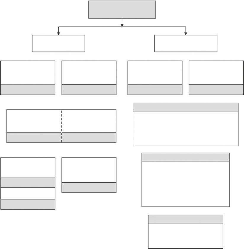
Since then, CEM regulations have expanded, affecting a wider range of sources and requiring a wider range of pollutants to be monitored. The basic CEM program elements established in the 1970s underlie most of the current regulations. The foundation of any regulatory continuous monitoring program incorporates three basic elements: (i) implementing rules, (ii) performance specifications, and (iii) quality assurance requirements. These three elements provide the necessary support for the application of CEM technology (Figure 2-1).
When placed on uneven surfaces of a wide range of industrial applications, agency regulatory policies must be robust enough to enable CEM systems to produce
accurate data. Continuing this analogy, when taking a photograph, a tripod serves to provide a stable base for a camera; the sharpness of the picture depends on the quality of the tripod as well as the quality of the camera. In the same sense, the quality of the data produced by a CEM system is dependent on both the system and the elements that support it.
Implementing rules address the source categories and types of units required to monitor emissions, whereas performance specifications provide design, installation, and certification criteria. Quality assurance (QA) requirements specify procedures necessary for obtaining accurate data on a continuing basis. These elements support a CEM program, and a failure in definition of any one element can lead to an ineffective or failed regulatory program. Each of these elements incorporates a number of integral parts, which are illustrated in Figure 2-2.
The regulatory development of implementing rules, performance specifications, and quality assurance
requirements are discussed later in this chapter. Details of performance specification, performance specification test procedures, and quality assurance programs are discussed in the dedicated chapters that follow.
IMPLEMENTING RULES IN THE UNITED STATES
Implementing rules specify the type of source affected by the rule and may further specify types of process units required to monitor emissions. For example, a Kraft pulp mill recovery furnace may be required to monitor opacity and total reduced sulfur (TRS), or a petroleum refinery sulfur recovery unit may be required to monitor SO2 and H2S emissions through an implementing rule.
The rule should also specify why monitoring is required – its purpose. This may not always be stated or may be ill-defined, particularly in permits. However, distinctions are important in the case of litigation. Purposes for which CEM systems are typically installed are as follows:
Control equipment operation and maintenance monitoring
Compliance monitoring
Emissions accounting
Public perception monitoring
The first U.S. Federal CEM implementing rules required the installation of CEM systems to monitor the performance of emissions control equipment. Since CEM systems provide a continuous record that shows if a source is either below or above its emissions limits (emissions
Elements of a CEM rule
standards), it was soon noted that the data could also be used for enforcement purposes. Implementing rules followed that required the installation of CEM systems to be used directly for enforcement. Another purpose for the installation of CEM systems is to provide the data necessary to support emissions accounting programs, such as the EPA acid rain program. Pollutant and flow monitoring data are used in these programs to calculate emissions in units of tons per year. A regulatory instrument called an “allowance” is equivalent to a right to emit one ton per year of a given pollutant and a source must have in its possession, the number of allowances equal its mass emissions expressed in tons/year. Here, CEM systems are the measurement tool used to track allowances.
Public perception monitoring (or more euphemistically, “good neighbor” monitoring) refers to more stringent monitoring requirements established for sources such as municipal and hazardous waste combustors. In this case, extensive monitoring requirements are specified, coupled with plant operational interlock criteria where waste feed is shut off if emission limits should be exceeded. The continual oversight given by this instrumentation is intended to provide assurances to the public that environmental concerns associated with these types of sources are being addressed.
In addition to addressing source categories, operational units, and monitoring purposes, implementing rules also specify source specific monitoring details, such as instrument span requirements, data conversion equations, averaging periods, quality assurance, and reporting requirements. These details are important for using the data, but are often overlooked, particularly in state permits. Although there is a greater awareness of the need to specify such requirements in the implementing rules, when they are not incorporated, the rule may be too ambiguous to fulfill its regulatory intent. The variety of implementing rules that require the installation of CEM systems are examined further in the following sections.
U.S. Federal Implementing Rules
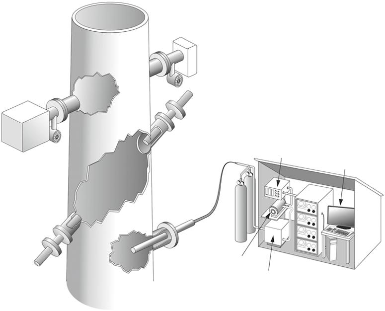
U.S. federal stationary source emissions standards and monitoring requirements are drafted by offices of the Environmental Protection Agency. The most important of these is the Office of Air Quality Planning and Standards (OAQPS), which developed the first CEM implementing rules and performance specifications in the early 1970s (U.S. EPA 1975). Other EPA offices have instituted CEM programs based on the original OAQPS regulations, modifying them for their own regulatory applications. Figure 2-3 summarizes CEM regulatory programs that have been instituted.
In the United States, rules are first developed by the respective office and proposed in the Federal Register (FR), a document published on each government busi-
ness day that includes regulatory proposals, promulgations, notices, and discussions concerning the rulemaking. After public hearings, comment, and revision, the regulations and requirements are promulgated and adopted into the U.S. Code of Federal Regulations (CFR). The CFR is a multivolume compendium of U.S. regulations for federal government agencies, which is revised annually to incorporate any new rules or changes in existing rules. It is the principle reference for environmental regulation in the United States.
Code of Federal Regulation citations are given in the format: (Title) CFR (Part). For example, 40 CFR 60 refers to the part of the code where the New Source Performance Standards (NSPS) are found. Performance specification test procedures for CEM systems are found in 40 CFR 60 Appendix B (U.S. EPA 2020c). Federal Register citations are given in the format: (Volume No.) FR (Page No.) (Date). As another example, the final performance specification test procedures 1–4 were published in the Federal Register in 1975 at 40 FR 46240 10/ 6/75. CFR publications can be found on http://www.ecfr. gov. Federal Register publications can be found on http:// www.govinfo.gov/app/collection/fr. Federal Register publications can be useful by providing a background behind decisions that went into a final rule. Preambles to final rules include EPA’s responses to comments submitted on the proposed rule on which the final rule is based. Most of the rules do not stand alone and refer to other rules, test methods, monitoring specifications, and quality assurance requirements in other subparts and/or appendices of the Code of Federal Regulations.
Once promulgated, implementing rules may be amended or superseded by subsequent rules. This can create some confusion, particularly when rules overlap, as has been the case with the acid rain rules of 40 CFR 75 and the New Source Performance Standards of 40 CFR 60. Because the source-specific standards are written at different times by different people, the formats, terminology, and specifications are sometimes inconsistent between the different standards. Although there are periodic attempts to harmonize the rules, inconsistencies often remain.
New Source Performance Standards, 40 CFR 60 U.S. EPA regulations concerning stationary sources are found under Title 40 Subchapter C of the Code. Newly constructed sources are required to meet New Source Performance Standards (NSPS), which are given in Part 60 of Title 40 (expressed as 40 CFR 60). Each source category, such as the electric utilities, municipal incinerators, or cement plants, is assigned a Subpart letter (Subpart Da, Eb, and F, respectively) by which it is referred to in the CFR (U.S. EPA 2020a).
The rules prepared by this office affect newly constructed sources. A “new source” is defined as one
New source performance standards (NSPS)
40 CFR 60
Rulemaking requiring CEM systems
Minimum emission monitoring requirements State agency programs
Cross state air pollution rule CSAPR
pollutants (NESHAPS) 40 CFR 51 App. P
40 CFR 61
Incineration standards hazardous waste
40 CFR 266
Sewage sludge
40 CFR 503?
CFR 63
greenhouse gas reporting rule 40 CFR 75
40 CFR 98
40 CFR 96
Permit programs
• Prevention of significant deterioration (PSD) 40 CFR 52
• Compliance assurance monitoring (CAM) (CEM Option) 40 CFR 64
• Other
State rulemaking and initiatives
Examples:
• RGGI/WSI (NE states carbon trading, CA carbon trading)
• RECLAIM (CA)
• PA requirements
• NH3 monitoring (NJ, VA, RI)
• HCI monitoring (CT, PA)
Discretionary programs
• Variances
• Orders
• Agreements
Figure 2-3 U.S. Rulemaking requiring CEM systems.
constructed after the date the rules are first proposed in the Federal Register. An “existing source” is a source constructed before that date. Rules for existing sources are given by the individual states, usually in facility operating permits, with federal guidance and approval. The Part 60 Subparts address primarily new sources, but also include subparts that provide guidance to the states to develop rules for existing sources. When meeting the federal guidance requirements, the rules for specific source categories can be incorporated into the State Implementation Plan (SIP) (U.S. EPA 2020b). Source categories required to install CEM systems under NSPS are given in Table 2-1.
Table 2-1 shows the depth of CEM applications in U.S. industry and power production, but it should also be viewed as a guide to the Part 60 Subparts. The table gives applicability dates that distinguish “existing”
sources from “new” and modified or reconstructed sources. The table lists those source categories required to monitor the concentration of gaseous pollutants, flue gas opacity, and/or particulate matter (PM). The table also lists the types of operational units on which a CEM system is to be installed. For example, Subpart BB for Kraft pulp mills may require monitoring on a number of devices, such as the recovery furnace, lime kiln, and digester contained within the plant. Sources such as the electric utilities or municipal waste combustors may have multiple boilers or combustors, all of which may require monitoring.
Note that most of the “effective dates” are old, and one might consider that “new” sources first affected by this program are now “old.” When Part 60 source requirements prove to be inadequate, new subparts are added to address newer “new” sources. This is the case
TABLE 2-1 (Continued)
Category Part 60 Subpart Affected Units Effective Datea,b
refineries Ja Fluid Catalytic Cracking Units Sulfur Recovery Units
a NSPS applies if construction commenced after this date.
b NSPS applies if modification or reconstruction commenced after this date.
c CEM requirements are as applicable when meeting the conditions of the subpart.
d Rule applies if constructed before this date.
e Organic monitoring device based on IP, photoionization, or thermal conductivity.
Source: Data from U.S. EPA (2020b).
for Subparts D and Da for electric utilities, Subparts Ea and Eb for municipal waste combustors, and Subparts J and Ja for petroleum refineries. The newer rules become more proscriptive and often require the installation of CEM systems not required in earlier subparts. Both new and existing stationary sources can be further regulated through programs such as the acid rain program of 40 CFR 75 and the air toxics program of 40 CFR 63, in addition to state permit requirements. Each of these programs can impose additional monitoring requirements.
Not listed in the table are operational units or smaller sources that instead of installing CEM systems may alternatively be required to monitor process parameters such as pressure drops, temperatures, or fuel flow rates. Regulatory relief is applied to smaller sources where it can be a burden to purchase, operate, and maintain a CEM system. Here, the less stringent parameter monitoring requirements for low-emitting sources may not be especially significant when considering their relatively smaller contribution to the atmospheric pollution burden.
The subparts tend to be complex. Accordingly, they should be referred to for detailed information concerning units of the emissions standards, monitoring requirements, reporting requirements, and exceptions.
General Provisions for the NSPS Subparts
General provisions pertinent to CEM systems required for sources regulated under the NSPS subparts are present in four sections of Part 60 of the Code. These sections are as follows:
§60.7 Notification and Recordkeeping
§60.8 Performance Tests
§60.11 Compliance with Standards and Maintenance Requirements
§60.13 Monitoring Requirements
Each of these sections gives important requirements regarding the opacity and gas monitoring systems mandated for source categories addressed by the subparts. These should be read in tandem with the subparts. For example, §60.7 gives requirements for Part 60 sources with installed CEM systems to submit excess emission reports and describes the information that is to be included in the report. In §60.8, requirements are given for conducting performance tests to determine whether the facility is within its compliance limits. Here, the performance tests conducted are those reference test methods of 40 CFR 60 Appendix A specified for the source category (e.g. acid plant, electric utility) (U.S. EPA 2020c).
Section 60.11 incorporates a requirement that has been central to U.S. EPA stationary source regulatory policy. This requirement [§60.11(d)] states:
At all times, including periods of startup, shutdown, and malfunction, owners and operators shall, to the extent practicable, maintain and operate any affected facility including associated air pollution control equipment in a manner consistent with good air pollution control practice for minimizing emissions. Determination of whether acceptable operating and maintenance procedures are being used will be based on information available to the Administrator which may include but is not limited to, monitoring results, opacity observations, review of operating and maintenance procedures, and inspection of the source.
This policy, formulated in the early 1970s, is reprised in the compliance assurance monitoring and credible evidence rules that resulted from congressional concerns addressed in the 1990 Clean Air Act Amendments (which is discussed below).
Section 60.13 incorporates important requirements for Part 60 CEM systems. This section is sometimes forgotten after a CEM program has been implemented, but nevertheless, contains essential program requirements. Among these requirements are given as follows:
• Performance Specification Tests. Part 60 installed systems must show that they meet performance specifications of 40 CFR 60 Appendix B (U.S. EPA 2020d) by conducting a performance specification test (Note: “performance specification tests” are used to certify CEM systems and are not the same as the “performance tests” of §60.8 conducted to determine source compliance with emission limits).
• Quality Assurance Requirements. In the absence of other quality assurance requirements, as a minimum; the system must conduct a zero and span drift check once every 24 hours, zero and span adjustments must be made if the drift exceeds twice the value of the drift performance specification of Appendix B, and the zero and span check procedures must be written.
• Representativeness. All CEM systems are to be installed such that measurements representative of actual emissions are obtained.
• Alternative Performance Test Requirements. An alternative to conducting reference method tests for determining relative accuracy may be requested if the pollutant emissions are less than 50% of the emissions limit (60.13(j)(1)). When applicable, this allows conducting a cylinder gas test (audit) (CGA) instead of a relative accuracy test audit (RATA).
NESHAP, 40 CFR 61 The National Emission Standards for Hazardous Air Pollutants (NESHAP), formerly legislated under Section 112 of the Clean Air Act, require continuous monitoring for a limited number of sources
covered under Part 61 of Title 40. As in Part 60, general monitoring instructions regarding notification, recordkeeping, etc. are given in the “general provisions” prior to the source requirements. Few pollutants were regulated under the NESHAP program due to uncertainties associated with risk assessments and scheduling mandates (Mohin 1992). Source categories affected by this subpart and monitoring requirements are discussed further in Chapter 13 on monitoring hazardous air pollutants.
The Air Toxics Program, 40 CFR 63 Title III of the 1990 Clean Air Amendments replaced the previous NESHAP program. Title III identified 189 hazardous air pollutants (HAPs) (later reduced to 187), to be regulated for sources emitting more than 10 tons/year of any one listed pollutant or 25 tons/year of a combination of listed pollutants. EPA has promulgated emission limits and engineering standards for the principal sources emitting HAPS (or “air toxics”). The sources must apply “maximum achievable control technology,” where MACT technology is the best control achieved in practice by 12% of the best controlled similar sources. However, MACT encourages process changes or other pollution prevention activities rather than the application of control equipment.
The air toxics, or “MACT standards,” also incorporate monitoring requirements to determine, on a continuous basis, whether emission limits are being met. Most MACT standards require parameter monitoring, in other words a “continuous parameter monitoring system (CPMS)” that is described in a “monitoring plan,” rather than the installation of CEM systems. However, where control devices are used that can be effectively monitored, such as carbon adsorbers and incinerators, CEM systems are either required or suggested as an alternative to parameter monitoring. The Part 63 Subparts give the emissions standards and monitoring requirements for HAPs emitted from 174 listed industries. Rather than requiring the monitoring of specific pollutants from the list of 187 HAPs, the use of surrogate analyzers is often allowed (such as a particulate monitor to monitor metal emissions or a total hydrocarbon monitor rather than a speciating instrument). Sources required to monitor HAPs and methods used to measure them are discussed further in Chapter 13.
Compliance Assurance Monitoring (CAM) 40 CFR
64 The compliance assurance monitoring program (CAM) was initiated from a congressional requirement included in the 1990 Clean Air Act Amendments (§702 (b) of the amendments). This amendment to Section 114 of the Clean Air Act states:
The Administrator shall in the case of any person which is the owner or operator of a major stationary source, and may in the case of any other person, require enhanced monitoring and submission of compliance certifications.
Compliance certifications shall include (A) identification of the applicable requirement that is the basis of the certification, (B) the method used for determining the compliance status of the source, (C) the compliance status of the source, (D) whether compliance is continuous or intermittent, (E) other such facts as the administrator may require.
The amendment addressed the concern of Congress that the compliance status of most emission sources was determined only periodically by conducting manual stack tests. It was viewed that since source operations may be highly tuned during such testing, operations may not necessarily be representative of day-to-day performance. Congress gave EPA the task to devise a strategy that can assure Congress (and the public) that emissions standards and limitations are being met continually, not just intermittently.
The Compliance Assurance Monitoring (CAM) rule was developed as a response to the requirement that essentially places the burden back upon the source. The CAM rule applies to sources required to obtain a Part 70 or 71 air permit and having emission units with active control devices, whose potential pre-control device emissions are at or above the emission thresholds that define a “major” source (such as 100 tons per year). Affected sources are to develop a “CAM Plan” that will provide assurance to the agency that they are meeting their emissions limitations (Neulicht et al. 1996). The CAM plan provides for the recording of work practice procedures, equipment monitoring, and inspection procedures related to pollution control compliance. CEM systems that measure pollutant emissions directly or by parameter monitoring techniques that provide indirect determinations may also be used. A guidance document on how to write a plan has been prepared by the U.S. EPA (OAQPS 1998).
Methods incorporated into the plan are to specify indicator ranges, within which the emission source is assumed to be in compliance. The range may be simply a range of pollutant concentration, or a range of pressure drops, temperatures, voltage settings, fuel flow, gas flows, and so on. Exceeding the range then triggers a requirement for initiating corrective action.
The CAM program emphasizes the use of plant sensors and parameter monitoring techniques to avoid the installation of CEM systems. This was due to public comment on an earlier “enhanced monitoring” rule intended to meet the requirements of §702 (b) of the 1990 CAA amendments. This earlier rule, viewed as a “CEM rule,” was withdrawn, due in part to outcry over assumed CEM system costs. However, the costs associated with developing CAM plans, modifying plans when plant operations change, and reporting parameter data may ultimately be comparable to the cost of CEM systems and process monitors. If a CEM system is already installed for compliance monitoring through a permit, NSPS, or other requirement, additional monitoring is not required.