Where can buy Geophysical monitoring for geologic carbon storage lianjie huang ebook with cheap pric
Geophysical Monitoring for Geologic Carbon Storage Lianjie Huang
Visit to download the full and correct content document: https://ebookmass.com/product/geophysical-monitoring-for-geologic-carbon-storage-li anjie-huang/
More products digital (pdf, epub, mobi) instant download maybe you interests ...
Geophysical Monitoring for Geologic Carbon Storage
Editor
Lianjie Huang
Geophysical Monitoring for Geologic Carbon Storage
Lianjie Huang, Los Alamos National Laboratory, USA
Storing carbon dioxide in underground geological formations is emerging as a promising technology to reduce carbon dioxide emissions in the atmosphere. A range of geophysical techniques can be deployed to remotely track carbon dioxide plumes and monitor changes in the subsurface, which is critical for ensuring for safe, long-term storage.
Geophysical Monitoring for Geologic Carbon Storage provides a comprehensive review of different geophysical techniques currently in use and being developed, assessing their advantages and limitations.
Volume highlights include:
• Geodetic and surface monitoring techniques
• Subsurface monitoring using seismic techniques
• Subsurface monitoring using non-seismic techniques
• Case studies of geophysical monitoring at different geologic carbon storage sites
The American Geophysical Union promotes discovery in Earth and space science for the benefit of humanity. Its publications disseminate scientific knowledge and provide resources for researchers, students, and professionals.
Geophysical Monograph Series
217 Deep Earth: Physics and Chemistry of the Lower Mantle and Core Hidenori Terasaki and Rebecca A. Fischer (Eds.)
218 Integrated Imaging of the Earth: Theory and Applications Max Moorkamp, Peter G. Lelievre, Niklas Linde, and Amir Khan (Eds.)
219 Plate Boundaries and Natural Hazards Joao Duarte and Wouter Schellart (Eds.)
220 Ionospheric Space Weather: Longitude and Hemispheric Dependences and Lower Atmosphere Forcing Timothy FullerRowell, Endawoke Yizengaw, Patricia H. Doherty, and Sunanda Basu (Eds.)
221 Terrestrial Water Cycle and Climate Change Natural and Human-Induced Impacts Qiuhong Tang and Taikan Oki (Eds.)
222 Magnetosphere-Ionosphere Coupling in the Solar System Charles R. Chappell, Robert W. Schunk, Peter M. Banks, James L. Burch, and Richard M. Thorne (Eds.)
223 Natural Hazard Uncertainty Assessment: Modeling and Decision Support Karin Riley, Peter Webley, and Matthew Thompson (Eds.)
224 Hydrodynamics of Time-Periodic Groundwater Flow: Diffusion Waves in Porous Media Joe S. Depner and Todd C. Rasmussen (Auth.)
225 Active Global Seismology Ibrahim Cemen and Yucel Yilmaz (Eds.)
226 Climate Extremes Simon Wang (Ed.)
227 Fault Zone Dynamic Processes Marion Thomas (Ed.)
228 Flood Damage Survey and Assessment: New Insights from Research and Practice Daniela Molinari, Scira Menoni, and Francesco Ballio (Eds.)
229 Water-Energy-Food Nexus – Principles and Practices P. Abdul Salam, Sangam Shrestha, Vishnu Prasad Pandey, and Anil K Anal (Eds.)
230 Dawn–Dusk Asymmetries in Planetary Plasma Environments Stein Haaland, Andrei Rounov, and Colin Forsyth (Eds.)
231 Bioenergy and Land Use Change Zhangcai Qin, Umakant Mishra, and Astley Hastings (Eds.)
232 Microstructural Geochronology: Planetary Records Down to Atom Scale Desmond Moser, Fernando Corfu, James Darling, Steven Reddy, and Kimberly Tait (Eds.)
233 Global Flood Hazard: Applications in Modeling, Mapping and Forecasting Guy Schumann, Paul D. Bates, Giuseppe T. Aronica, and Heiko Apel (Eds.)
234 Pre-Earthquake Processes: A Multidisciplinary Approach to Earthquake Prediction Studies Dimitar Ouzounov, Sergey Pulinets, Katsumi Hattori, and Patrick Taylor (Eds.)
235 Electric Currents in Geospace and Beyond Andreas Keiling, Octav Marghitu, and Michael Wheatland (Eds.)
236 Quantifying Uncertainty in Subsurface Systems Celine Scheidt, Lewis Li, and Jef Caers (Eds.)
237 Petroleum Engineering Moshood Sanni (Ed.)
238 Geological Carbon Storage: Subsurface Seals and Caprock Integrity Stephanie Vialle, Jonathan Ajo-Franklin, and J. William Carey (Eds.)
239 Lithospheric Discontinuities Huaiyu Yuan and Barbara Romanowicz (Eds.)
240 Chemostratigraphy Across Major Chronological Eras Alcides N. Sial, Claudio Gaucher, Muthuvairavasamy Ramkumar, and Valderez Pinto Ferreira (Eds.)
241 Mathematical Geoenergy: Discovery, Depletion, and Renewal Paul Pukite, Dennis Coyne, and Daniel Challou (Eds.)
242 Ore Deposits: Origin, Exploration, and Exploitation Sophie Decree and Laurence Robb (Eds.)
243 Kuroshio Current: Physical, Biogeochemical and Ecosystem Dynamics Takeyoshi Nagai, Hiroaki Saito, Koji Suzuki, and Motomitsu Takahashi (Eds.)
244 Geomagnetically Induced Currents from the Sun to the Power Grid Jennifer L. Gannon, Andrei Swidinsky, and Zhonghua Xu (Eds.)
Geophysical Monograph Series
245 Shale: Subsurface Science and Engineering Thomas Dewers, Jason Heath, and Marcelo Sánchez (Eds.)
246 Submarine Landslides: Subaqueous Mass Transport Deposits From Outcrops to Seismic Profiles Kei Ogata, Andrea Festa, and Gian Andrea Pini (Eds.)
247 Iceland: Tectonics, Volcanics, and Glacial Features Tamie J. Jovanelly
248 Dayside Magnetosphere Interactions Qiugang Zong, Philippe Escoubet, David Sibeck, Guan Le, and Hui Zhang (Eds.)
249 Carbon in Earth’s Interior Craig E. Manning, Jung-Fu Lin, and Wendy L. Mao (Eds.)
250 Nitrogen Overload: Environmental Degradation, Ramifications, and Economic Costs Brian G. Katz
251 Biogeochemical Cycles: Ecological Drivers and Environmental Impact Katerina Dontsova, Zsuzsanna Balogh-Brunstad, and Gaël Le Roux (Eds.)
252 Seismoelectric Exploration: Theory, Experiments, and Applications Niels Grobbe, André Revil, Zhenya Zhu, and Evert Slob (Eds.)
253 El Nino Southern Oscillation in a Changing Climate Michael J. McPhaden, Agus Santoso, and Wenju Cai (Eds.)
254 Dynamic Magma Evolution Francesco Vetere (Ed.)
255 Large Igneous Provinces: A Driver of Global Environmental and Biotic Changes Richard. E. Ernst, Alexander J. Dickson, and Andrey Bekker (Eds.)
256 Coastal Ecosystems in Transition: A Comparative Analysis of the Northern Adriatic and Chesapeake Bay Thomas C. Malone, Alenka Malej, and Jadran Faganeli (Eds.)
257 Hydrogeology, Chemical Weathering, and Soil Formation Allen Hunt, Markus Egli, and Boris Faybishenko (Eds.)
258 Solar Physics and Solar Wind Nour E. Raouafi and Angelos Vourlidas (Eds.)
259 Magnetospheres in the Solar System Romain Maggiolo, Nicolas André, Hiroshi Hasegawa, and Daniel T. Welling (Eds.)
260 Ionosphere Dynamics and Applications Chaosong Huang and Gang Lu (Eds.)
261 Upper Atmosphere Dynamics and Energetics Wenbin Wang and Yongliang Zhang (Eds.)
262 Space Weather Effects and Applications Anthea J. Coster, Philip J. Erickson, and Louis J. Lanzerotti (Eds.)
263 Mantle Convection and Surface Expressions Hauke Marquardt, Maxim Ballmer, Sanne Cottaar, and Jasper Konter (Eds.)
264 Crustal Magmatic System Evolution: Anatomy, Architecture, and Physico-Chemical Processes Matteo Masotta, Christoph Beier, and Silvio Mollo (Eds.)
265 Global Drought and Flood: Observation, Modeling, and Prediction Huan Wu, Dennis P. Lettenmaier, Qiuhong Tang, and Philip J. Ward (Eds.)
266 Magma Redox Geochemistry Roberto Moretti and Daniel R. Neuville (Eds.)
267 Wetland Carbon and Environmental Management Ken W. Krauss, Zhiliang Zhu, and Camille L. Stagg (Eds.)
268 Distributed Acoustic Sensing in Geophysics: Methods and Applications Yingping Li, Martin Karrenbach, and Jonathan B. Ajo-Franklin (Eds.)
269 Congo Basin Hydrology, Climate, and Biogeochemistry: A Foundation for the Future Raphael M.Tshimanga, Guy D. Moukandi N’kaya, and Douglas Alsdorf (Eds.)
270 Muography: Exploring Earth’s Subsurface with Elementary Particles László Oláh, Hiroyuki K. M.Tanaka, and Dezső Varga (Eds.)
271 Remote Sensing of Water-Related Hazards Ke Zhang, Yang Hong, and Amir AghaKouchak (Eds.)
272 Geophysical Monitoring for Geologic Carbon Storage Lianjie Huang (Ed.)
Geophysical Monograph 272
Geophysical Monitoring for Geologic Carbon Storage
Lianjie Huang
Editor
This Work is a co-publication of the American Geophysical Union and John Wiley and Sons, Inc.
All rights reserved. No part of this publication may be reproduced, stored in a retrieval system, or transmitted, in any form or by any means, electronic, mechanical, photocopying, recording or otherwise, except as permitted by law. Advice on how to obtain permission to reuse material from this title is available at http://www.wiley.com/go/permissions.
Published under the aegis of the AGU Publications Committee
Matthew Giampoala, Vice President, Publications
Carol Frost, Chair, Publications Committee
For details about the American Geophysical Union visit us at www.agu.org.
The right of Lianjie Huang to be identified as the editor of this work has been asserted in accordance with law.
Registered Office
John Wiley & Sons, Inc., 111 River Street, Hoboken, NJ 07030, USA
Editorial Office
111 River Street, Hoboken, NJ 07030, USA
For details of our global editorial offices, customer services, and more information about Wiley products visit us at www.wiley.com.
Wiley also publishes its books in a variety of electronic formats and by print-on-demand. Some content that appears in standard print versions of this book may not be available in other formats.
Limit of Liability/Disclaimer of Warranty
While the publisher and authors have used their best efforts in preparing this work, they make no representations or warranties with respect to the accuracy or completeness of the contents of this work and specifically disclaim all warranties, including without limitation any implied warranties of merchantability or fitness for a particular purpose. No warranty may be created or extended by sales representatives, written sales materials or promotional statements for this work. The fact that an organization, website, or product is referred to in this work as a citation and/or potential source of further information does not mean that the publisher and authors endorse the information or services the organization, website, or product may provide or recommendations it may make. This work is sold with the understanding that the publisher is not engaged in rendering professional services. The advice and strategies contained herein may not be suitable for your situation. You should consult with a specialist where appropriate. Further, readers should be aware that websites listed in this work may have changed or disappeared between when this work was written and when it is read. Neither the publisher nor authors shall be liable for any loss of profit or any other commercial damages, including but not limited to special, incidental, consequential, or other damages.
Library of Congress Cataloging-in-Publication Data
Names: Huang, Lianjie, editor.
Title: Geophysical monitoring for geologic carbon storage / edited by Lianjie Huang.
Description: Hoboken, NJ : Wiley-American Geophysical Union, 2022. | Includes bibliographical references and index.
Identifiers: LCCN 2021059926 (print) | LCCN 2021059927 (ebook) | ISBN 9781119156833 (cloth) | ISBN 9781119156857 (adobe pdf) | ISBN 9781119156840 (epub)
LC record available at https://lccn.loc.gov/2021059926
LC ebook record available at https://lccn.loc.gov/2021059927
Cover Design: Wiley
Cover Image: Kevin Eaves/Shutterstock
Set in 10/12pt Times New Roman by Straive, Pondicherry, India
10 9 8 7 6 5 4 3 2 1
and Surface Monitoring 2 Geodetic Monitoring of the Geological Storage of Greenhouse Gas Emissions
Donald Vasco, Alessandro Ferretti, Alessio Rucci, Giacomo Falorni, Sergey Samsonov, Don White, and Magdalena Czarnogorska
3 Surface Monitoring, Verification, and Accounting (MVA) for Geologic Sequestration Storage Samuel Clegg, Kristy Nowak-Lovato, Robert Currier, Julianna Fessenden, and Ronald Martinez
Seismic Response of Fractured Sandstone During Geological Sequestration of CO2: Laboratory Measurements at Mid (Sonic) Frequencies and X-Ray CT
and Attenuation: Rhyolite and Carbonate Examples
13 Tracking Subsurface Supercritical CO2 Using Advanced Reflection Seismic and Well Log-Based Workflows Incorporating Fluid Density and Pore Pressure Effects: Relevance to Reservoir Monitoring and CO2 EOR
Alan Mur, Thomas M. Daley, and William Harbert
Part III Subsurface Nonseismic Monitoring
14 Monitoring Carbon Storage Sites With Time-Lapse Gravity Surveys
Delphine Appriou and Alain Bonneville ......................................................................................................
15 Fundamentals of Electrical and Electromagnetic Techniques for CO2 Monitoring
Erika Gasperikova and H. Frank Morrison ...................................................................................................
16 Monitoring Geologic Carbon Sequestration Using Electrical Resistivity Tomography
Xianjin Yang and Charles Carrigan
17 Monitoring of Large-Scale CO2 Injection Using CSEM, Gravimetric, and Seismic AVO Data
Svenn Tveit and Trond Mannseth
18 Self-Potential Monitoring for Geologic Carbon Dioxide Storage
Yuji Nishi and Tuneo Ishido
Part IV Case Studies of Geophysical Monitoring
19 Microseismic Monitoring, Event Location, and Focal Mechanisms at the Illinois Basin–Decatur Project, Decatur, Illinois, USA
Robert A. Bauer, Robert Will, George El-Kaseeh, Paul Jaques, Sallie Greenberg, and Michael Carney
20 Associated Storage With Enhanced Oil Recovery: A Large-Scale Carbon Capture, Utilization, and Storage Demonstration in Farnsworth, Texas, USA
Balch and Brian McPherson .............................................................................................................
21 Testing Geophysical Methods for Assessing CO2 Migration at the SECARB Early Test, Cranfield, Mississippi, USA
22 Toward Quantitative CO2 Monitoring at Sleipner, Norway
Anouar Romdhane, Bastien Dupuy, Etor Querendez, and Peder
23 Geophysical Monitoring of CO2 Injection at Ketzin, Germany
Peter Bergmann, Magdalena Diersch, Julia Götz, Monika Ivandic, Alexandra Ivanova, Christopher Juhlin, Juliane Kummerow, Axel Liebscher, Stefan Lüth, Sjef Meekes, Ben Norden, Cornelia Schmidt-Hattenberger, Florian Wagner, and Fengjiao Zhang
24 Geophysical Monitoring Techniques: Current Status and Future Directions
LIST OF CONTRIBUTORS
Delphine Appriou
Pacific Northwest National Laboratory Richland, Washington, USA
Robert Balch
Petroleum Recovery Research Center New Mexico Institute of Mining and Technology Socorro, New Mexico, USA
Robert A. Bauer
Illinois State Geological Survey University of Illinois at Urbana-Champaign Champaign, Illinois, USA
Peter Bergmann ROSEN Technology and Research GmbH Lingen, Germany
Alain Bonneville
Pacific Northwest National Laboratory Richland, Washington, USA and College of Earth, Ocean and Atmospheric Sciences Oregon State University Corvalis, Oregon, USA
David W. Bowen
Department of Earth Sciences Montana State University Bozeman, Montana, USA
Michael Carney Greenway Technical Consulting Services, Inc. Houston, Texas, USA
Charles Carrigan
Atmospheric, Earth, and Energy Division Lawrence Livermore National Laboratory Livermore, California, USA
Ting Chen
Geophysics Group
Los Alamos National Laboratory Los Alamos, New Mexico, USA
Samuel Clegg
Chemistry Division
Los Alamos National Laboratory Los Alamos, New Mexico, USA
Vincent Clochard
IFP Energies Nouvelles Paris, France
Dustin Crandall Leidos Corporation
National Energy Technology Laboratory
U.S. Department of Energy Pittsburgh, Pennsylvania, USA
Robert Currier
Chemistry Division
Los Alamos National Laboratory Los Alamos, New Mexico, USA
Magdalena Czarnogorska
Canada Centre for Mapping and Earth Observation Natural Resources Canada Ottawa, Ontario, Canada
Thomas M. Daley
Energy Geoscience Division Lawrence Berkeley National Laboratory Berkeley, California, USA
Daniel Delaney Department of Physics College of Natural Sciences and Mathematics University of Alaska Fairbanks, Alaska, USA
Huseyin Denli Geophysics Group
Los Alamos National Laboratory Los Alamos, New Mexico, USA
Bryan DeVault Vecta Oil & Gas Ltd. The Woodlands, Texas, USA
Magdalena Diersch
Centre for Geological Storage
GFZ German Research Centre for Geosciences Potsdam, Germany
Bastien Dupuy
Applied Geoscience Group
SINTEF Industry
Trondheim, Norway
Peder Eliasson
Applied Geoscience Group
SINTEF Industry Trondheim, Norway
George El-Kaseeh
GSNA Consulting Services, Inc. Klein, Texas, USA
Giacomo Falorni TRE Altamira Inc. Vancouver, British Columbia, Canada
Alessandro Ferretti
TRE ALTAMIRA Srl Milan, Italy
Julianna Fessenden
Earth and Environmental Sciences
Los Alamos National Laboratory Los Alamos, New Mexico, USA
Erika Gasperikova Energy Geosciences Division
Lawrence Berkeley National Laboratory Berkeley, California, USA
Kai Gao Geophysics Group Los Alamos National Laboratory Los Alamos, New Mexico, USA
Julia Götz Centre for Geological Storage GFZ German Research Centre for Geosciences Potsdam, Germany
Sallie Greenberg Illinois State Geological Survey University of Illinois at Urbana-Champaign Champaign, Illinois, USA
Igor Haljasmaa Leidos Corporation
National Energy Technology Laboratory
U.S. Department of Energy Pittsburgh, Pennsylvania, USA
William Harbert
Oak Ridge Institute for Science and Education
National Energy Technology Laboratory Pittsburgh, Pennsylvania, USA and Department of Geology and Environmental Science University of Pittsburgh Pittsburgh, Pennsylvania, USA
Susan D. Hovorka Gulf Coast Carbon Center Bureau of Economic Geology
Jackson School of Geosciences
The University of Texas at Austin Austin, Texas, USA
Hui Huang Geophysics Group Los Alamos National Laboratory Los Alamos, New Mexico, USA
Lianjie Huang Geophysics Group
Los Alamos National Laboratory Los Alamos, New Mexico, USA
Tuneo Ishido
Research Institute for Geo-Resources and Environment Geological Survey of Japan National Institute of Advanced Industrial Science and Technology Ibaraki, Japan
Monika Ivandic Department of Earth Sciences Uppsala University Uppsala, Sweden
Alexandra Ivanova Centre for Geological Storage
GFZ German Research Centre for Geosciences Potsdam, Germany
Paul Jaques Schlumberger Cambridge, UK
Christopher Juhlin
Department of Earth Sciences
Uppsala University Uppsala, Sweden
Timothy Kneafsey
Earth and Environmental Sciences
Lawrence Berkeley National Laboratory Berkeley, California, USA
Juliane Kummerow
Centre for Geological Storage
GFZ German Research Centre for Geosciences Potsdam, Germany
Axel Liebscher
Centre for Geological Storage
GFZ German Research Centre for Geosciences Potsdam, Germany
Youzuo Lin
Geophysics Group
Los Alamos National Laboratory Los Alamos, New Mexico, USA
Stefan Lüth
Centre for Geological Storage
GFZ German Research Centre for Geosciences Potsdam, Germany
Trond Mannseth
NORCE Norwegian Research Centre AS Bergen, Norway
Ronald Martinez Chemistry Division Los Alamos National Laboratory Los Alamos, New Mexico, USA
Brian McPherson Energy and Geoscience Institute University of Utah Salt Lake City, Utah, USA
Sjef Meekes TNO Utrech, The Netherlands
H. Frank Morrison
University of California at Berkeley Berkeley, California, USA
Alan Mur
Ikon Science Ltd Houston, Texas, USA
Seiji Nakagawa
Earth and Environmental Sciences
Lawrence Berkeley National Laboratory Berkeley, California, USA
Yuji Nishi
Research Institute for Geo-Resources and Environment Geological Survey of Japan National Institute of Advanced Industrial Science and Technology Ibaraki, Japan
Ben Norden
Centre for Geological Storage
GFZ German Research Centre for Geosciences Potsdam, Germany
Kristy Nowak-Lovato Chemistry Division
Los Alamos National Laboratory Los Alamos, New Mexico, USA
Christopher Purcell CNOOC International Houston, Texas, USA
Etor Querendez
Applied Geoscience Group SINTEF Industry Trondheim, Norway
Anouar Romdhane Applied Geoscience Group SINTEF Industry Trondheim, Norway
Alessio Rucci TRE ALTAMIRA Srl Milan, Italy
Sergey Samsonov
Canada Centre for Mapping and Earth Observation
Natural Resources Canada Ottawa, Ontario, Canada
Cornelia Schmidt-Hattenberger Centre for Geological Storage
GFZ German Research Centre for Geosciences Potsdam, Germany
Xuefeng Shang Geophysics Group
Los Alamos National Laboratory Los Alamos, New Mexico, USA
Yee Soong
Leidos Corporation
National Energy Technology Laboratory
U.S. Department of Energy Pittsburgh, Pennsylvania, USA
Lee H. Spangler
Energy Research Institute
Montana State University Bozeman, Montana, USA
Sirui Tan
Geophysics Group
Los Alamos National Laboratory Los Alamos, New Mexico, USA
Svenn Tveit
NORCE Norwegian Research Centre AS Bergen, Norway
Donald Vasco
Energy Geosciences Division
Lawrence Berkeley National Laboratory Berkeley, California, USA
Florian Wagner Department of Geophysics
Steinmann Institute University of Bonn Bonn, Germany
Yi Wang Geophysics Group
Los Alamos National Laboratory Los Alamos, New Mexico, USA and
Laboratory of Seismology and Physics of Earth’s Interior School of Earth and Space Sciences University of Science and Technology of China Hefei, China
Don White
Geological Survey of Canada
Natural Resources Canada Ottawa, Ontario, Canada
Robert Will
WRG Subsurface Consulting LLC Littleton, Colorado, USA
Xianjin Yang
Atmospheric, Earth, and Energy Division
Lawrence Livermore National Laboratory Livermore, California, USA
Fengjiao Zhang
Department of Earth Sciences
Uppsala University Uppsala, Sweden
Zhifu Zhang
Geophysics Group
Los Alamos National Laboratory Los Alamos, New Mexico, USA and
School of Geophysics and Information Technology
China University of Geoscience Beijing, China
Zhigang Zhang
Geophysics Group
Los Alamos National Laboratory Los Alamos, New Mexico, USA
PREFACE
Geologic carbon storage is the storage of carbon dioxide, generally in supercritical form, in underground geological formations. This kind of underground storage is emerging as a promising technology for dealing with increasing concentrations of carbon dioxide in Earth’s atmosphere. Ensuring safe and long-term CO2 storage in different subsurface settings requires site characterization and monitoring during and post-CO2 injection. A range of geophysical monitoring techniques can be deployed in this regard, to remotely track subsurface CO2 plumes and to monitor fracture/fault zones (one of the primary leakage paths), caprock integrity, and mineralogical changes. This book provides a comprehensive reference to different geophysical techniques currently used and being developed for monitoring geologic carbon storage and for assessing their advantages and limitations.
The book is divided into four parts, three describing different monitoring methods and techniques and one presenting case studies from around the world. Part I contains two chapters on geodetic and surface monitoring techniques, specifically Interferometric Synthetic Aperture Radar (InSAR) and frequency modulated spectroscopy. Part II looks at subsurface monitoring using seismic techniques, including optimal design for cost-effective monitoring using microseismic networks and time-lapse active seismic surveys; offset, walkaway, and 3D vertical seismic profiling (VSP) monitoring/imaging; quantifying time-lapse changes of subsurface geophysical properties; site characterization using multicomponent seismic data; and workflows for determining fluid and pressure effects resulting from a supercritical CO 2 injection in a sandstone reservoir using 4D reflection seismic data and well logs. Part III looks at subsurface monitoring
using nonseismic techniques with chapters on timelapse gravity surveys; electrical and electromagnetic techniques; electrical resistivity tomography; integrated controlled source electromagnetic (CSEM), gravimetric, seismic amplitude-versus-offset (AVO) monitoring; and self-potential monitoring. Finally, Part IV presents five case studies of geophysical monitoring at different geologic carbon storage sites. The first three are in the United States: the Illinois Basin-Decatur Project in Decatur, Illinois; Phase III of the Southwest Partnership on Carbon Sequestration in Farnsworth, Texas; and the Southeast Regional Sequestration Partnership project in Cranfield, Mississippi. Two further examples are presented from Europe: the Sleipner project in Norway, and the CO2 injection project at Ketzin in Germany.
I thank all the authors for their contributions and numerous reviewers for their careful review of the chapter manuscripts. Appreciation also goes to AGU and Wiley for their support during the preparation and production of this book. Particularly, I thank Dr. Estella Atekwana from the AGU Books Editorial Board and the AGU Publications Director, Dr. Jenny Lunn, for helpful feedback on the manuscript. I also express gratitude to staff at Wiley, including Dr. Rituparna Bose, Emily Bae, Kathryn Corcoran, Poornima Devi, Layla Harden, Karthiga Mani, Nithya Sechin, Bobby Kilshaw, Carol Kromminga, Angela Cohen, Shiji Sreejish, and Bhavani Ganesh Kumar for their support.
Lianjie Huang
Los Alamos National Laboratory, USA
1
Evaluating Different Geophysical Monitoring Techniques for Geological Carbon Storage
Lianjie Huang1 and Xianjin Yang2
ABSTRACT
Various geophysical techniques can be used to monitor geologic carbon storage and ensure that it is safe in the long term. Seismic methods are often used to monitor CO2 migration in the deep regions of a geologic carbon storage site while nonseismic methods provide complementary monitoring from shallow subsurface to the surface. This chapter gives an overview of the geophysical monitoring methods presented in this book including Interferometric Synthetic Aperture Radar (InSAR), frequency modulated spectroscopy, induced microseismic monitoring, time-lapse active seismic monitoring, gravity, electrical and electromagnetic techniques, controlled-source electromagnetic method, electrical resistivity tomography (ERT), and self-potential measurements.
1.1. INTRODUCTION
Geologic carbon storage, or geologic carbon sequestration, is an emerging technology to permanently store or sequester separated and captured anthropogenic carbon dioxide (CO2) from industrial sources into deep geologic formations. Some large-scale anthropogenic CO2 sources include coal-fired or gas-fired power plants, oil and gas refineries, steel mills, and cement plants. The purpose of geologic carbon storage is to mitigate the rising CO2 concentration in Earth’s atmosphere and to substantially reduce its impact on the global warming.
Geophysical monitoring is crucial for ensuring safe, long-term geologic carbon storage. A geologic carbon storage project requires site characterization before CO2 injection to evaluate if the site is suitable for geologic carbon storage, and monitoring of CO2 migration during and after CO2 injection. Various geophysical monitoring
1 Geophysics Group, Los Alamos National Laboratory, Los Alamos, New Mexico, USA
2 Atmospheric, Earth, and Energy Division, Lawrence Livermore National Laboratory, Livermore, California, USA
techniques can remotely track subsurface CO2 plumes and provide crucial information to mitigate potential leakage risks. A geologic carbon storage project should integrate complementary geophysical monitoring techniques to form a comprehensive monitoring plan because various geophysical monitoring techniques have their own advantages and limitations. Joint analyses of information from different geophysical monitoring techniques can increase the monitoring confidence. Monitoring plans must be adaptable during different phases of a geologic carbon storage project from site characterization to injection to postinjection site care. The type of monitoring technique that should be deployed also depends on the monitoring targets, such as the atmosphere, drinking water aquifers, cap rock, and storage formation.
This book provides a comprehensive reference to different geophysical techniques currently used and being developed for monitoring geologic carbon storage, and assesses their advantages and limitations. Part I introduces two techniques for geodetic and surface monitoring. Part II is on subsurface monitoring using seismic techniques. Part III focuses on subsurface monitoring using nonseismic
Geophysical Monitoring for Geologic Carbon Storage, Geophysical Monograph 272, First Edition. Edited by Lianjie Huang.
techniques. Part IV presents five case studies of geophysical monitoring at different worldwide geologic carbon storage sites.
The field of geophysical monitoring for geologic carbon storage is rapidly growing. Many new technologies are being developed. This book does not aim to include all possible geophysical monitoring technologies but rather presents an overview of current techniques and their applications, drawing on examples from geologic carbon storage sites across the world.
1.2. GEODETIC AND SURFACE MONITORING
Geodetic monitoring, including global positioning system (GPS) monitoring, tilt and Interferometric Synthetic Aperture Radar (InSAR), measures displacements and strains, both on the surface and within the interior of the Earth. Space-based InSAR is perhaps the most cost-effective geodetic technique for remote monitoring of land-based geologic carbon storage sites.
CO2 injection might cause Earth’s surface to deform. Geodetic monitoring is a cost-effective approach to monitoring reservoir integrity and detecting possible CO2 leakage. The technique involves repeated measurements of the deformation of Earth’s surface. In Chapter 2, Vasco et al. present a geodetic monitoring technique using InSAR. InSAR, which provides high spatial resolution and broad surface coverage, is particularly suitable for monitoring large-scale geologic carbon storage. Multi-temporal analysis can improve the accuracy of surface displacement measurements. Data interpretation and inversion techniques may be used to relate the observed surface displacements to the CO2 injectioninduced volume change at depth. Some advantages of geodetic monitoring include: (1) observations are usually frequent in time, from every few minutes to every few months; (2) geodetic measurements are often conducted remotely, simplifying data collection and enabling costeffective monitoring; (3) geodetic observations are sensitive to fluid volume and pressure changes associated with geologic carbon storage; and (4) geodetic monitoring may be able to detect CO2 leakage and the upward migration of fluid under pressure because the magnitude of surface displacement increases dramatically when the fluid-injection-induced defor mation approaches the surface. InSAR monitoring has been successfully used at a gas storage site at In Salah, Algeria, where it has been determined that the flow in the reservoir was influenced by large-scale fault/fracture zones. InSAR monitoring at the Aquistore CO2 storage project in Canada and the Illinois Basin Decatur Project in the United States indicates no major surface deformation that might be attributed to stored carbon dioxide. InSAR can possibly monitor ground deformation with an accuracy of 0.5 cm.
InSAR data quality may be compromised by diverse land surface environments and unfavorable site conditions, such as mining and construction activities, groundwater recharge, swelling clays, and slope instabilities.
Surface monitoring is used to detect CO2 on the surface when some of the injected CO2 migrates to the surface. Most surface monitoring techniques involve monitoring absolute changes in bulk CO2 concentration, which is complicated by the diurnal cycle. In Chapter 3, Clegg et al. present a surface monitoring technique using frequency modulated spectroscopy, which uses changes in the carbon stable isotope ratio in CO2 to distinguish anthropogenic and natural CO2. Passive and active absorption spectroscopy can measure the absolute concentration of atmospheric CO2 and derive seepage from the sequestration site using changes from the background diurnal concentrations. Absorption spectroscopy has the advantage of both point source in situ analysis and wide area remote analysis of the area above a geologic carbon storage site.
1.3. SUBSURFACE SEISMIC MONITORING
Seismic monitoring can use active seismic surveys and/ or microseismic events induced by CO2 injection and migration. Microseismic monitoring uses sensors/geophones deployed on the surface covering the monitoring region, and/or sensors/geophones in one or more boreholes to monitor induced microseismic events smaller than what surface seismic arrays can detect. For costeffective microseismic monitoring, we need to understand how many sensors/geophones are needed, and how to distribute them spatially to monitor targets of interest, such as the CO2 storage reservoir, caprock, faults, and so on. In Chapter 4, Chen and Huang present a methodology to determine the optimal number of geophones using a surface seismic monitoring network or a borehole geophone array for cost-effective monitoring of target regions. They determine the optimal number of seismic stations based on the trade-off curve of the event location accuracy versus the total number of seismic stations. They design an optimal microseismic monitoring network based on widely accepted guiding principles, and the relationship between the location accuracy of microseismic events and the total number of seismic stations. The method is based on the trade-off curve between the mean location accuracy and the number of seismic stations. In practical applications, three-component geophones can provide more useful information of shear-wave signals to improve microseismic monitoring compared with one-component geophones.
Active seismic monitoring uses time-lapse seismic reflection/transmission data. The underlining physical principle of this monitoring technique is based on the effects of
(supercritical) carbon dioxide on subsurface elastic parameters. CO2 injection and migration alter elastic parameters such as compressional and shear velocities, density, and seismic attenuations in isotropic geologic formations, and also anisotropic parameters in anisotropic geologic formations. Studies of rock physics on the effects of CO2 injection and migration form the foundation of timelapse seismic monitoring for geologic carbon storage. In Chapter 5, Nakagawa and Kneafsey present laboratory measurements of the seismic response of fractured sandstone during geologic carbon sequestration. They employ a modified resonant bar technique to make laboratory measurements, and give the dynamic Young’s modulus, shear modulus, and attenuation in core samples with supercritical CO2 injected, within a sonic frequency band of ~1 kHz to ~2 kHz. They use X-ray CT to understand the distribution of supercritical CO2 injected into the core samples. Their laboratory experiment results show that changes in seismic-wave velocities and attenuations strongly depend on the fracture orientation. In Chapter 6, Delaney et al. use laboratory ultrasonic experiments to study rock physics properties of rhyolite and carbonate samples, and the effects of pressure, temperature, porosity, and fluid saturation on their rock properties. In their experiments, they vary the pore-filling fluids, effective pressures, and temperatures. They find that the framework composition, porosity, heterogeneities, temperature, effective pressure and pore-filling fluids are first-order controls on trends in elastic parameters and wave attenuation. Their findings could provide insight on using amplitude versus offset (AVO) for seismic monitoring. Their results show that the quality factor of compressional waves measuring compressional-wave attenuation is inversely proportional to rock porosity and is weakly dependent on temperature. These results reveal the relationships of the ultrasonic velocity and the quality factor as a function of both temperature and effective pressure.
Time-lapse 3D seismic monitoring, or 4D seismic monitoring, is considered as the most effective tool for 3D subsurface monitoring of CO2 injection and migration. However, time-lapse 3D seismic surveys and data processing are costly and time consuming. For the similar purpose of optimal design of a microseismic monitoring network, Gao et al. in Chapter 7 introduce a numerical method for designing optimal time-lapse seismic monitoring surveys by analyzing sensitivities of elastic waves in isotropic and anisotropic media with respect to reservoir geophysical property changes. Conventional seismic surveys are designed based on seismic-wave illumination of the entire subsurface imaging region, and require a large number of sources and receivers to produce high-resolution images of the subsurface. By contrast, time-lapse seismic monitoring is
not designed to image the entire subsurface region, but only the target monitoring regions, such as the CO2 storage reservoir, caprock, and faults. Therefore, timelapse seismic monitoring needs only seismic information from such regions, rather than from the entire subsurface region. The optimal design of time-lapse seismic surveys is based on elastic-wave sensitivity analysis, that is, numerical modeling of elastic-wave changes with respect to changes of geophysical properties within target monitoring regions. The method numerically solves the elastic-wave sensitivity equations obtained by differentiating the elastic-wave equations with respect to geophysical parameters, such as density, compressional- and shear-wave velocities, and saturation parameters, in isotropic and anisotropic media. Receivers should be placed in surface regions for surface seismic surveys or borehole locations for vertical seismic profiling (VSP) surveys with significant values of elastic-wave sensitivity energies. The number of receivers needed for cost-effective timelapse seismic monitoring is only a fraction of a regular 3D seismic survey.
The 3D surface seismic monitoring has the advantage of monitoring a large subsurface area to track CO2 migration in the 3D space. However, seismic imaging/monitoring resolution decreases with the depth, particularly for CO2 storage at geologic formations at several kilometers in depth. Compared with surface seismic monitoring, VSP monitoring improves seismic imaging/monitoring resolution in the deep region when receivers are placed in the deep region of the subsurface. The image resolution of VSP monitoring is usually twice that of surface seismic monitoring. The limitation of VSP monitoring is that the lateral monitoring range is smaller than surface seismic monitoring.
VSP surveys use active seismic sources at various offset locations (offset VSP), or along various walkway lines from the monitoring well (walkaway VSP), or using a 2D surface source distribution (3D VSP). Offset VSP monitoring uses only a few offset source points, and has the lowest cost among the three different types of time-lapse VSP survey. However, offset VSP can monitor only in the sparse azimuthal directions along a monitoring well to offset source directions. 3D VSP monitoring is the most expensive among the three VSP monitoring approaches, with the highest spatial coverage of the monitoring region. The walkaway VSP monitoring is the trade-off between the offset VSP monitoring and 3D VSP monitoring.
In Chapter 8, on offset VSP monitoring, Zhang and Huang study the capability of offset VSP imaging for monitoring CO2 injection/migration, and present monitoring results at the Aneth CO2-EOR (Enhanced Oil Recovery) field in Utah. The offset VSP monitoring uses a permanent geophone string with 60 levels and 96
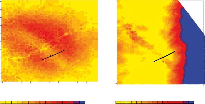
channels cemented into a monitoring well. Because of uncertainties in the offset VSP source locations during repeat VSP surveys, they present a method to use travel times of the downgoing VSP waves and double-difference tomography to invert for the “true” VSP source locations. This approach addresses the source repeatability issue in practical offset VSP monitoring. Zhang and Huang apply wave-equation migration imaging of the preprocessed and balanced time-lapse offset VSP data from the Aneth CO2-EOR field and the inverted “true” VSP source locations to infer the reservoir changes. To reduce the imaging noise of the offset VSP data, they employ an angledomain imaging condition with reflection angle constraint for different offset VSP data sets to produce time-lapse migration images, showing reservoir changes caused by CO2 injection/migration along different offset directions are different, indicating an anisotropic CO2 migration pattern relative to the injection wells.
In Chapter 9 on walkaway VSP monitoring, Wang et al. apply reverse-time migration (RTM) to time-lapse walkaway VSP data acquired at the SACROC CO2-EOR field in Scurry County, Texas, USA, to reveal changes in the reservoir caused by CO2 injection and migration. Before they apply RTM to the data, they perform statics correction and amplitude balancing to the time-lapse walkaway VSP data sets. To mitigate the image artifacts caused by the limited subsurface seismic illumination of the walkaway VSP surveys, they analyze and process the RTM images in the angle domain to greatly improve the image quality.
Because of limited seismic illumination of VSP surveys, migration imaging of VSP data often contains significant image artifacts, which can be alleviated using an angle-domain imaging condition. This alleviation is tedious if not impossible for 3D VSP data. 3D leastsquares reverse-time migration (LSRTM) is an alternative approach to addressing such a problem. To demonstrate the improved imaging capability of 3D LSRTM of 3D VSP data, Tan et al., in Chapter 10, apply the method to a portion of the 3D VSP data acquired at the Cranfield CO2-EOR field in Mississippi, USA, for monitoring CO2 injection to obtain a high-resolution 3D subsurface image. LSRTM solves for a reflectivity model by minimizing the difference between the observed data and modeled data. The advantages of LSRTM over RTM of VSP data include: (1) LSRTM significantly improves the spatial resolution of the layer images, and (2) LSRTM extends the horizontal imaging region to areas that cannot be imaged using RTM.
Besides time- lapse seismic imaging, quantifying changes of subsurface geophysical properties caused by CO2 injection/migration can provide crucial information of CO2 plumes. In Chapter 11, Lin et al. present a doubledifference seismic-waveform inversion method to jointly
invert time-lapse seismic data for reservoir changes of elastic parameters. Inverting individual time-lapse seismic data sets separately may result in significant inversion artifacts and inaccurate inversion results. Doubledifference acoustic- or elastic-waveform inversion constrains time-lapse seismic data sets with each other to improve the robustness of inversion of time-lapse changes and reduce inversion artifacts. In Lin et al.’s doubledifference seismic-waveform inversion methods, they employ an energy-weighted preconditioner, a spatial priori information (target monitoring regions), and a modified total-variation regularization scheme to improve the inversion accuracy of changes of subsurface geophysical properties. They validate the method using time-lapse walkaway VSP data acquired at the SACROC CO2-EOR field, and reveal the velocity decrease in the geologic formation where CO2 was injected.
Multicomponent seismic surveys acquire not only compressional-wave signals, but also shear-wave signals that carry useful information for high-resolution subsurface site characterization and monitoring. When using shear-wave sources, the multicomponent seismic surveys record the full nine-component elastic wavefields, which are the most complete seismic data. Such data contain compression-to-compression and shear-to-shear waves in addition to converted waves including compression-toshear and shear-to-compression waves. Multicomponent seismic data are far more sensitive to fracture zones than compressional-wave data, allowing improved characterization/monitoring of potential leakage pathways or preferential flow directions compared with onecomponent data. In Chapter 12, on site characterization using multicomponent seismic data, DeVault et al. describe joint inversion of multicomponent seismic data for deriving elastic parameters from multicomponent data and demonstrate the unique advantages for geophysical CO2 reservoir characterization. They present results of joint inversion for characterizing the Duperow CO2-bearing zone at Kevin Dome, Montana, USA. They demonstrate that the additional amplitude and polarization information contained in multicomponent data allows for the estimation of shear impedance, density, and azimuthal anisotropic parameters with much greater accuracy than using compressional-wave seismic data.
In Chapter 13, Mur et al. develop forward modeling workflows for predicting fluid and pressure effects resulting from supercritical CO2 (scCO2) injection in a sandstone reservoir using 4D reflection seismic data and well logs. They use a 3D prestack seismic data set, two 3D seismic poststack volumes, and a wireline log from the sandstone reservoir, to perform forward modeling and predict reservoir seismic response of fluid substituted CO2 as a component of the pore-filling fluid mix in a reservoir unit. They use time-lapse 3D seismic data acquired
before and after CO2 injection and postinjection common midpoint stacks to determine regions of possible fluid density and pore pressures signatures. The lateral changes in amplitude versus offset (AVO) can be an indicator of pore-filling fluid changes. They implement the AkiRichards method to model reflected wave amplitudes at increasing offset angles on time-lapse prestack seismic data from the Cranfield Field, Mississippi, USA. They present results on the effects of seismic-wave reflectivity caused by the injection of CO2 in a sandstone reservoir at Cranfield, and predict the fluid effects of CO2 presence in the reservoir by applying fluid substitutions to produce reservoir property models and compare these effects with an actual 4D seismic survey.
1.4. SUBSURFACE NONSEISMIC MONITORING
Migration of CO2 at a geologic carbon storage site causes subsurface mass redistribution. Lower density CO2 displaces higher density brine, which results in reduction of the bulk formation density. Time-lapse gravity monitoring is sensitive to the bulk density changes. Gravity sensors can be deployed on the ground surface or in a borehole or on the seafloor. When CO2 is present at a subsurface depth of greater than 700 m, CO2 exists in a supercritical state and its density ranges from 0.25 to 0.70 g/cm3. The density contrast between brine and CO2 in a CO2 storage site is often less than 0.5 g/cm3
In Chapter 14, Appriou and Bonneville introduce the gravity method and discuss its modeling and application to various geologic carbon storage sites. Detection of gravity variations accompanying mass redistributions in the subsurface caused by fluid movements in reservoirs provides a unique means to monitor the dynamics of a carbon sequestration site. With the recent advancement in instrument capabilities, the gravity method provides a promising monitoring technique.
Because a CO2 storage reservoir is often located at a large depth and spatial resolution of gravity surveys decreases with the depth, there are often limited applications that land surface gravity surveys can provide. To improve the plume resolution, a gravimeter must be located closer to a CO2 plume, either in a borehole or on the seafloor for an offshore geologic carbon storage site. There have been only two gravity monitoring applications at commercial-scale CO2 storage sites. A seafloor gravity monitoring survey was performed at the Sleipner CO2 storage site in Norway. The high repeatability of 1.1–4.3 μGal in gravity measurements was achieved in a dynamic seafloor environment. Hydrocarbon production is another source of reservoir density change and complicates the gravity interpretation. The gravity anomaly reached tens of μGal after injection of 18 MMT CO2
Gravity monitoring estimated that the mass of CO2 in the storage reservoir agrees with the injected CO2 mass without leakage.
Compared with seismic monitoring, gravity monitoring is more cost-effective and may be deployed between repeated seismic surveys if the model predicts a measurable gravity response. Downhole and seafloor gravity monitoring of deep CO2 storage is more effective than surface gravity surveys, which may be better suited for monitoring shallow CO2 leakage.
The injection of carbon dioxide results in increased resistivity, which may be detected by electrical and EM imaging techniques, such as electrical resistivity tomography, complex resistivity method, magnetotelluric method, controlled source EM, and other EM methods. In Chapter 15, Gasperikova and Morrison present the electrical and electromagnetic (EM) techniques to map the electrical resistivity of the subsurface for monitoring CO2 injection and migration. Both surface and borehole resistivity methods are relatively insensitive to horizontal resistive layers of CO2 plumes. Monitoring with electromagnetic sources at depth shows great promise for detecting and monitoring the emplacement of tabular zones or bodies of resistive CO2. Surfacebased EM techniques with an induction coil source are not suitable for detection of CO2 plumes deeper than 1,000 m.
Electrical and EM methods can be used to monitor CO2 leakage into the shallow geologic formations. Gasphase CO2 increases the bulk electrical resistivity. On the other hand, brine leakage and dissolved CO2 in groundwater decrease the electrical resistivity. Electrical and EM monitoring should account for both effects of fluid salinity and CO2 saturation.
Electrical resistivity tomography (ERT) is an alternative high-resolution technique for the shallow aquifer and deep reservoir monitoring. In Chapter 16, Yang and Carrigan describe the ERT method for tracking migration of a supercritical CO2 plume in a deep storage reservoir and for detecting CO2 leakage in a shallow aquifer. With downhole electrodes close to the target of interest, ERT can characterize the temporal and spatial resistivity changes effectively. A resistive supercritical CO2 plume displaces conductive brine and increases the bulk resistivity of storage formation. However, brine leakage and CO2 dissolution in a shallow aquifer lower the bulk resistivity of the formation. They present two case histories to demonstrate the capability of ERT that provides daily tomographic images of CO2 distribution, which complements temporally sparse wireline logs and cross-well seismic data. The surface ERT method is effective for monitoring shallower than 100 m in depth. The primary challenge of cross-well ERT is the high cost of using two or more closely spaced monitoring wells to deploy vertical electrode arrays. Single-well ERT may be used when closely spaced monitoring wells are not available.
The controlled source electromagnetic (CSEM) method is mostly an offshore monitoring technique using electromagnetic remote-sensing technology to map the electric resistivity distribution of the subsurface. In Chapter 17, Tveit and Mannseth introduce a Bayesian sequential inversion methodology for combining geophysical data types of different resolutions. They first use CSEM or gravimetric data to invert for a low-resolution result, which is used as prior information for inversion of seismic amplitude-versus-offset (AVO) data to improve resolution. The unknown geophysical parameters, for example, electric conductivity, density, and seismic velocity, are represented using a carefully designed parameterization based on the level-set framework, which allows for representation of region boundaries defined by the large-scale CO2 plume and slowly varying geophysical properties inside and outside the CO2 plume. They show that seismic AVO inversion results are improved with the sequential inversion methodology using prior information from either CSEM or gravimetric inversion.
Fluid flow through a porous media can generate electrical potential gradient or streaming potential along the flow path. The self-potential (SP) technique is a passive electrical monitoring method that measures spontaneous or natural electrical potential from the subsurface. In Chapter 18, Nishi and Ishido introduce the SP monitoring technique. Two SP mechanisms are studied with numerical simulations. The electrokinetic coupling mechanism produces SP caused by changing reservoir conditions such as pressure disturbance from results of reservoir simulation. The geobattery mechanism creates a galvanic cell caused by subsurface electrochemical conditions near a metallic well casing. CO2 injection alters deeper reducing environment and redox potential, which results in an SP anomaly. If a substantial amount of CO2 migrates upward into a shallow fresh water aquifer through a vertical fault and creates substantial pressure disturbances, observable self-potential measurements caused by electrokinetic coupling would provide a costeffective monitoring method for CO2 leakage detection. They observed a local self-potential increase near the wellhead of an injection well associated with CO2 injection at the Aneth oil field in southeastern Utah, USA.
1.5. CASE STUDIES OF GEOPHYSICAL MONITORING
In Chapter 19, Bauer et al. present a case study of microseismic monitoring at the Illinois Basin Decatur Project of the Midwest Geological Sequestration Consortium. The project site is located in east-central Illinois in the north-central area of the Illinois Basin in the midcontinent region of the United States. For over
three years, the project safely injected nearly 1.1 million tons of supercritical carbon dioxide into the base of a 500-m thick saline sandstone reservoir at a depth of 2.14 km. They collected a unique data set encompassing an extensive quantity of microseismic and concurrent operational monitoring data before, during, and after injection operations, and presented results of microseismic event location and focal mechanisms. They demonstrate the compatibility of technical and operational activities under evolving and challenging conditions.
In Chapter 20, Balch and McPherson present an overview of the Phase III of the Southwest Partnership on Carbon Sequestration (SWP) in Farnsworth, Texas, USA. The project has completed its injection period with the storage of over 700,000 tonnes of CO2 at an active commercial-scale CO2-EOR field. They summarize the interrelationship of monitoring activities, the status of postinjection monitoring, and the optimization required to maximize storage while providing the greatest oil production incentive to the field operator, among others.
In Chapter 21, Hovorka gives an experimental study of testing and assessing geophysical monitoring methods for tracking CO2 migration during large volume injection at the Southeast Regional Sequestration Partnership project in Cranfield, Mississippi, USA. The project uses several geophysical tools to detect CO2 in the injection zone, including time-lapse 3D seismic, 3D VSP, time-lapse cross-well seismic, electrical resistance tomography, borehole gravity, time-lapse wireline sonic, pulsed neutron logging, and fluid density logging. The experiment reveals the strengths and weaknesses of different monitoring methods. Interference among different monitoring tools is significant. The site operator should avoid deploying as many tools as possible, but rather select best tools for the job and deployment condition. Monitoring data play an important role in calibrating the reservoir model.
In Chapter 22, Romdhane et al. describe a case study on quantitative monitoring at Sleipner in Norway. They evaluate a methodology combining high-resolution seismic-waveform tomography and rock physics inversion for monitoring the CO2 plume at Sleipner. They show that using multiparameter seismic inversion or multiphysics integration of data can lead to a better discrimination between the different effects of CO2 injection/migration on rock physics properties and reduce inversion uncertainties.
Finally, in Chapter 23, Bergmann et al. present an overview of geophysical monitoring of CO2 injection at Ketzin in Germany. They describe seismic measurements and electrical resistivity tomography performed during the period of site development and CO2 injection. They find that a combination of several geophysical methods is preferred.
ACKNOWLEDGMENTS
This work was supported by the U.S. Department of Energy (DOE) through the Los Alamos National Laboratory (LANL) operated by Triad National Security, LLC, for the National Nuclear Security Administration (NNSA) of U.S. DOE under Contract No. 89233218CNA000001, and through Lawrence Livermore
National Laboratory (LLNL) under Contract DE-AC5207NA27344. We thank the AGU Publications Director Dr. Jenny Lunn and Dr. Estella Atekwana of the AGU Books Editorial Board for their careful review and valuable comments. We also thank David Li of LANL for his review. This chapter is approved for public release by LANL (LA-UR-21-27246) and by LLNL (LLNL-BOOK-824879).
Part I Geodetic and Surface Monitoring
2
Geodetic Monitoring of the Geological Storage of Greenhouse Gas Emissions
Donald
Vasco1, Alessandro Ferretti2, Alessio Rucci2, Giacomo Falorni3, Sergey Samsonov4, Don White5, and Magdalena Czarnogorska4
ABSTRACT
Geodetic monitoring involves the repeated measurement of the deformation of the Earth. As discussed here, it is a cost-effective approach for inferring reservoir integrity and detecting possible leakage associated with the geological storage of greenhouse gas emissions. Most geodetic methods have favorable temporal sampling, from minutes to months depending upon the technique adopted, and can detect anomalous behavior in a timely fashion. Satellite-based approaches such as Interferometric Synthetic Aperture Radar (InSAR), with their high spatial resolution and broad coverage, are particularly well suited for monitoring industrial-scale storage efforts. Multitemporal analysis, such as permanent scatterer techniques, are improving the accuracy of surface displacement measurements to better than 4 – 5 mm. New satellites, including the recent X-band systems, are allowing for the routine estimation of two components of deformation. Data interpretation and inversion techniques may be used to relate the observed displacements to injection-related volume change at depth. InSAR monitoring was used successfully at a gas storage site at In Salah, Algeria, where it was determined that the flow in the reservoir was influenced by large-scale fault/fracture zones. InSAR observations are also key components of the monitoring programs at the Aquistore CO2 storage project in Canada, and the Illinois Basis Decatur Project in the United States. Current InSAR data from both sites indicate no major surface deformation that might be attributed to the stored carbon dioxide, suggesting that the injected fluid remains at depth.
2.1. INTRODUCTION
1Energy Geosciences Division, Lawrence Berkeley National Laboratory, Berkeley, California, USA
2 TRE ALTAMIRA Srl, Milan, Italy
3 TRE Altamira Inc., Vancouver, British Columbia, Canada
4 Canada Centre for Mapping and Earth Observation, Natural Resources Canada, Ottawa, Ontario, Canada
Geodetic monitoring, the repeated measurement of displacements and strains, both on the surface and within the interior of the Earth, provides an important class of techniques for assuring the safety of geological storage and for detecting leakage. There are important advantages associated with geodetic methods. The observations are usually gathered frequently in time, from every few minutes to every few months, depending upon the type of data. There are a diverse set of instruments for measuring strain and displacement in various configurations, either on the Earth’s surface, at depth, or even from space. Thus, geodetic measurement may often be gather remotely, greatly simplifying data collection and allowing for costeffective monitoring, particularly in comparison with more intrusive techniques such as seismic surveys. The Earth often deforms in response to fluid injection, particularly at the volumes and rates associated with the geological storage of carbon dioxide. Therefore, geodetic observations
Geophysical Monitoring for Geologic Carbon Storage, Geophysical Monograph 272, First Edition. Edited by Lianjie Huang.
are sensitive to fluid volume and pressure changes and may be used to monitor the fate of injected fluids. The magnitude of surface displacement increases dramatically as the source driving the deformation approaches the surface. Thus, geodetic monitoring is well suited to detecting leakage and the upward migration of fluids under pressure. In this chapter, we will discuss the use of geodetic data for monitoring injected carbon dioxide. Our primary focus will be on space-based Interferometric Synthetic Aperture Radar (InSAR) as this is perhaps the most cost-effective geodetic technique for land-based storage sites.
2.2. OBSERVATIONAL METHODS
2.2.1. Overview
Given its practical applications, geodesy, the measurement of distances and changes in distances (displacements), is probably one of the oldest scientific disciplines. Early leveling work and distance-measuring techniques involving the use of calibrated rods and chains date back to ancient times and continue to this day, though they have largely been replaced by satellite-based and laserbased techniques. Another early technique was the measurement of the local slope, the horizontal gradient of surface elevation, using a calibrated bubble level. This has evolved to modern day, highly accurate, capacitancebased tilt meters, capable of determining angular changes with nanoradian precision (Wright, 1998), optical fibertilt meters (Chawah et al., 2015), and portable tilt meters and extensometers (Hisz et al., 2013). Advanced tilt meters are now self leveling and may be used in boreholes and on the seabed. Trilateration by a constellation of satellites is the basis for the Global Positioning System (GPS), and Global Navigation Satellite Systems (GNSS) in general. This technology appears in many applications including the monitoring of subsurface fluid flow (Moreau & Dauteuil, 2013). Both tilt and GNSS measurements usually have high temporal resolution, with observations gathered every few minutes or hours (Schuite et al., 2017). However, cost often constrains one to a sparse network of instruments, limiting the spatial resolution of the displacement field. Leveling is similarly restricted to point measurements, typically gathered along roads or other open areas.
There is another class of observation techniques that can best be described as scanning systems. In these devices, propagating waves are reflected off objects of interest and the returns are used to estimate distances. Most commonly, electromagnetic waves are utilized. However, there are also sonar (sound waves) and seismic (elastic waves) systems that are used in particular applications. For example, time-lapse seismic surveys have been used to extract seismic time strains over deforming
reservoirs, a measure of the vertical strain in the subsurface. Such a technique has the advantage that the wave is sensing displacements at depth and even within the reservoir. Such displacements will typically be much larger than surface displacements. Shortly after the invention of the laser, the phase shift of its signal was used to measure changes in distance. Such laser ranging has progressed and is now used over a wide range of scales from engineering applications to airborne LiDAR surveys and even satellites (Eitel et al., 2016) and is useful for mapping geologic hazards (Joyce et al., 2014). Longer wavelength microwave signals are used in InSAR imaging, perhaps the most promising geodetic technology for monitoring the geological storage of carbon dioxide (Massonnet & Feigl, 1998; Rosen et al., 2000; Ferretti, 2014). In the next section, we describe this approach in much more detail. In Field Applications, section 2.4, we illustrate the use of InSAR observations at three storage sites.
2.2.2. SAR Interferometry
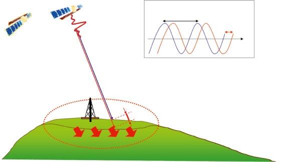
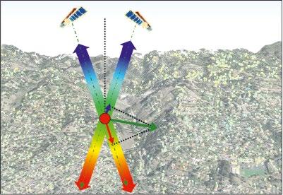
Radar sensors, mounted on satellite platforms, airplanes, or even a tripod on the ground, make it possible to measure ground displacement with millimeter accuracy, thanks to a particular technique known as SAR (Synthetic Aperture Radar) interferometry (InSAR) (see Ferretti, 2014, for a comprehensive review). The satellites both send and receive signals, recording the complex returns and using them for both imaging and range (distance) estimation (Fig. 2.1). Unlike optical systems, the sensors operate in the microwave domain, with wavelengths of a few centimeters, 100,000 times longer than those of the visible spectrum. Being an active system, a radar sensor can function 24 hours a day and year-round, as it can see through clouds, fog, and rain, independent of the Earth’s illumination.
An important feature of a SAR system is its ability to record both amplitude and phase information. While the amplitude depends on the amount of energy backscattered toward the sensor, the phase is related to the distance between the phase center of the radar antenna and the target on ground. More precisely, the phase value φ of a pixel P of a radar image can be modeled as a mixture of four distinct contributions (Ferretti et al., 2007a):
Pr an 4 , (2.1)
where ϑ is the phase shift related to the location and to the reflectivity of all elementary scatterers within the resolution cell associated with pixel P. The coefficient 4 r is the most significant contribution in any geodetic
Figure 2.1 A schematic showing the relationship between ground displacement and signal phase shift. The numeric value of the wavelength, λ, is that used by the ERS satellites operated by the European Space Agency (ESA).
application, as it is associated with the sensor-to-target distance r. The term a is a delay introduced by the medium (the Earth’s atmosphere) that the electromagnetic wave propagates through. This quantity, known as the atmospheric phase screen (APS), is often the main source of noise and can compromise the quality of any distance estimate. The last term, n, is a phase contribution related to system noise (thermal noise, quantization, etc.).
The phase values contained in a single SAR image are of little practical use, as it is impossible to separate the different contributions in equation (2.1), at least without prior information. The basic idea of SAR interferometry is to measure the phase change, or interference, over time, between two radar images, generating an interferogram I:
Pr an 4 (2.2)
If we consider an idealized situation where the noise is negligible, the surface character (reflectivity) and atmospheric conditions are constant between the two SAR acquisitions, then equation 2.2 reduces to
explains why interferometric SAR techniques can measure range variations with high sensitivity: the unit of length of the measurement is the wavelength (a few centimeters long) rather than the range resolution of the radar sensor (typically a few meters). A displacement of the radar target by a distance of λ/2 will create a phase shift of 2π radians. Therefore, a range variation of just 1 mm creates a phase shift of more than 20 degrees between two SAR images acquired in the X-band (λ = 3 cm), which can be easily detected.
A direct approach, involving the computation of phase variations on a pixel-by-pixel basis between two radar images, can be used successfully only if the reflective character of the radar target does not change over time, the signal-to-noise-ratio (SNR) is high enough, and the atmospheric phase components are negligible. When this is not the case, the analysis of a single interferogram is not sufficient to produce useful estimates and a multiinterferogram approach is required. In fact, the analysis of long temporal series of SAR images, as described in the next subsection, is perhaps the best way to disentangle the different phase contributions and retrieve highquality displacement data.
2.2.3 Multitemporal Analysis
Therefore, if a point on the ground moves during the time interval between the acquisition of the two radar images with similar geometry, the distance between the sensor and the target changes, creating a phase shift proportional to the displacement (Fig. 2.1). Equation (2.3)
Techniques utilizing a suite of interferograms, multiinterferogram approaches, are aimed at overcoming limitations associated with phase decorrelation and atmospheric effects. The PSInSAR technique (Ferretti et al., 2000, 2001), developed in the late nineties, initiated a “second generation” of algorithms addressing the
I
I
difficulties related to conventional (single-pair) analyses. The basic idea is to compare many SAR images and to focus the analysis on high-quality radar targets, usually referred to as permanent scatterers (PS). Such targets exhibit very stable radar signatures and allow the implementation of powerful filtering procedures to estimate and remove atmospheric disturbances, so that extremely accurate displacement data can be estimated. Common to all geodetic applications, the displacements are computed with respect to a stable reference point.
A recent enhancement of the permanent scatterer technique, the SqueeSAR algorithm (Ferretti et al., 2011), allows for two families of stable points on the Earth’s surface, permanent scatterers and distributed scatterers. As noted above, permanent scatterers (PS) are radar targets that are highly reflective (backscatter significant energy), generating very bright pixels in a SAR scene. Permanent scatterers are associated with stable features such as buildings, metallic objects, pylons, antennae, outcrops, and so on. Distributed scatterers (DS) are radar targets usually composed of a localized collection of pixels in the SAR image, all exhibiting a very similar radar signature. Such scatterers usually correspond to rocky areas, detritus, and areas generally free of vegetation. Temporal decorrelation, though still present in distributed scatterers, is small enough to allow for the retrieval of their displacements. Provided enough SAR images are available, one can determine a time series of range change (displacement along the line of sight) regardless of the type of scatterer identified by the algorithm. Thus, estimates of the geographic coordinates of the measurement point (located with a precision of about 1 m), average annual velocity of the measurement point (with a precision dependent on the number of data available, but typically less than 1 mm/yr), and time-series of scatterer displacement (with a precision typically better than 4 – 5 mm for individual measurements).
In order to successfully perform a multi-interferogram analysis, a minimum number of satellite images (approximately 10 – 15) are required. This is necessary to create a reliable statistical analysis of the radar returns, making it possible to identify pixels that can be used in the analysis. The higher the number of images acquired and processed, the better the quality of the results. For displacement data associated with permanent and distributed scatterers, a key factor is the distance from the reference point. The relative accuracy can be better than a few millimeters for a distance less than the average correlation length of the atmospheric components (about 4 km at midlatitudes). Average displacement rates can be estimated with a precision better than 1 mm/yr, depending on the number of data available and the temporal span of the acquisitions (Ferretti, 2014).
2.2.4 Two-Dimensional Displacement Decomposition
Satellite SAR interferometry measures only the projection of the three-dimensional displacement vector along the satellite line of sight. The data from any given interferogram are, therefore, single component distance measurements. However, it is possible to combine radar data acquired from different acquisition geometries to approximate two-dimensional displacement fields (Rucci et al., 2013). In fact, all SAR sensors follow near-polar orbits and every point on Earth can be imaged by two different acquisition geometries: one with the satellite flying from north to south (descending mode), looking westward (for right-looking sensors) and the other with the antenna moving from south to north (ascending mode), looking eastward. This is the reason why, by combining InSAR results from both acquisition modes, it is possible to estimate two components of displacement.
To illustrate how the decomposition is performed, imagine a Cartesian reference system where the three axes correspond to the East-West (X), North-South (Y), and Vertical (Z) directions. Consider the case in which two estimates of the target range change are available, obtained from both ascending and descending radar acquisitions, namely r a and rd (Fig. 2.2). In the Cartesian reference system X-Y-Z, the range change of a scatterer on ground can be expressed as:
where d x, d y, and d z represent the component of the displacement d along the E-W, N-S, and Vertical directions, and l x, l y, l z are the direction cosines of the look vector.
Given our knowledge of the satellite orbit, the line of sight of the radar antenna is known, as are the
Figure 2.2 Example of motion decomposition combining ascending and descending acquisition geometry.
corresponding direction cosines of the velocity vector r a and rd. It is thus possible to write the following system of equations:
where l x, a, l y, a, l z, a, and l x, d, l y, d, l z, d are the direction cosines of the satellite line of sight for both ascending and descending acquisitions. The problem is poorly posed if we now want to invert for the full three-dimensional velocity vector, as there are three unknowns (d x, d y, and d z) and only two equations. However, because the satellite orbit is almost circumpolar, the sensitivity to possible motion in the north-south direction is usually very small (the direction cosines l y, a and l y, d are close to 0). This allows us to rewrite the system in the following form:
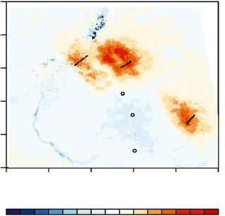
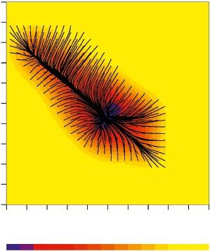
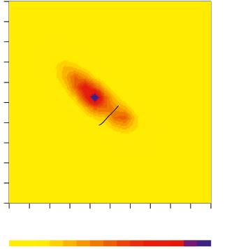
layer, then it is important to include the impermeable boundaries of the layer. Or, if the injected fluid induces the opening of a tensile fracture, then the strike and dip of the feature will need to be specified, perhaps by a datafitting procedure. For a tensile fracture, the volume change is completely determined by the aperture change over the fracture. Thus, the nature of the elemental source will be different from the volume expansion of a grid block. In fact, the expansion of a grid block can be modeled by three orthogonal tensile fractures, one along each axis. Other, more complicated source combinations are possible, such as slip induced along a tensile fracture. A correct formulation of the problem requires knowledge of the geology as well as of the general stress conditions at depth. Furthermore, one must be willing to modify the formulation in light of new information. For example, at In Salah, a double-lobed pattern of surface deformation indicated a tensile feature at depth, giving rise to a modified source model.
an equation that may be solved for d x and d z
2.3. DATA INTERPRETATION AND INVERSION METHODS
When a volume of fluid is introduced under pressure at some depth within the Earth, it changes the state of rockfluid system around the injection site. The nature of the change is determined by the temperature, composition, pressure, and flow rate of the fluid and the initial conditions within the host formation. Generally, the injected fluid will displace the in-situ fluid, leading to pressure and, consequently, volume changes that depend on the compressibility of the system as a whole. These volume changes will lead to strain within the Earth that will be transmitted outward from the injection site, ultimately reaching the Earth’s surface. Given sufficient strain at depth, the resulting surface displacement can be large enough to produce a significant signal, observable by modern geodetic instruments such as a SAR satellite. Such signals can produce valuable information concerning the source of the deformation.
Given an observable pattern of surface deformation, one can attempt to infer properties of the source generating the deformation. That is, one can invert the observed data to estimate parameters describing the source. One of the most important aspects of an inversion for volume change is how the source model is parameterized. In order to effectively represent the source, one must know its basic geometrical properties and boundary conditions. For example, if the injected fluid is confined to a porous
Under favorable circumstances, surface deformation may be used to image the migration of the injected and displaced fluid at depth and the geological features that are controlling it. Needless to say, making such inferences will require knowledge of the properties of the fluids involved and of the overburden. However, the nature of the injected fluid is usually well known and the structure and properties of the overburden are also constrained by seismic data and well logs. One does not typically inject fluid blindly into the Earth. For the sake of our discussion, we will assume that the Earth behaves elastically at a sufficient distance from the source and for the time intervals in question, a few months to a few years. Furthermore, we will assume that the elastic properties can be reasonably estimated from the available data. Other rheological models, such as viscoelasticity, are certainly possible and are not a barrier to the approach that we shall lay out here. However, for the conditions associated with the geological storage of greenhouse gases, an elastic overburden is a reasonable model.
Geodetic methods do not really allow us to image fluid flow directly. In particular, displacements at the surface and within the overburden are responding to the effective volume changes induced by fluid injection and withdrawal. Imagine a box around that part of the reservoir influenced by fluid injection or withdrawal. If we cut out the reservoir and simply applied the same displacements as those caused by the fluid flow to the boundaries of the box, the resulting deformation in the overburden, and on the surface, would be the same. So, in reality, one can solve only for such effective displacements or volume changes. Other assumptions, such as constitutive laws for the reservoir, are required if we are to interpret the volume changes in terms of fluid pressure changes, thermal expansion, or nonelastic processes. Therefore, we will
formulate our inversion in terms of reservoir fractional volume change in order to minimize the number of assumptions that must be invoked.
In an elastic Earth, the displacement at the surface, and in the overburden, is linearly related to the volume changes within the source region (Aki & Richards, 1980; Vasco et al., 1988). Thus, one can write the calculated displacements as an integral over with source volume V as
For InSAR observations, the data will consist of rangechange values, given by the projection of the displacement vector onto the satellite look vector l = (l1, l2, l3). Thus, the range change will be given by r = l u and the projection applied to equation 2.9 gives
where Δv(y) is the fractional volume change at source location y. The quantity Gi(x, y) is a Green’s function representing the i-th displacement component at location x that results from a point volume increase at y. The Green’s function encapsulates the physics of the propagation of elastic deformation from the source to the observation point, obtained by solving the governing equation with a point source. For a simple medium with sufficient symmetry, such as a homogeneous half-space, it is possible to produce an analytic Green’s function. For a more general medium, one must resort to numerical approaches in order to compute Gi(x, y). Even a layered medium requires a numerical approach to compute the Green’s function (Wang et al., 2006).
Equation (2.7) constitutes the forward problem whereby the injected volume is specified and the displacement at the observation points is calculated. For computational purposes, the source volume is usually decomposed into a discrete sum of N elementary volumes, such as rectangular grid blocks, and the total volume has the basis function representation
If we write the collective range-change data for all of the pixels as a vector r, then the corresponding set of linear constraints, each in the form of equation 2.11, may be written as a matrix equation
In the inverse problem, observational data are used to estimate the distribution of volume change at depth. The most common approach is a least-squares formulation in which one seeks a model v that minimizes the sum of the square of the residuals
Note that the volumes may be taken to be quite small and sources are often decomposed into one or more point-like sources. Substituting the volume expansion (2.8) into the integral 2.7, and using the linearity of integration, results in the expression
While it is possible to try to estimate the volume change for a full three-dimensional source model by minimizing S, the solution will most likely be nonunique or poorly determined. That is, there will be many possible solutions and solving the least-squares constraint equations will not lead to a stable answer. One can stabilize the solution by adding penalty terms to the misfit function S, representing aspects of the model that are considered undesirable, a procedure known as regularization. For example, the magnitude of deviations from an initial or prior model,
It is assumed that the fractional volume change given by Δυi is constant over the elemental volume Vj. The function Gij(x) represents the integral of the Green’s function Gi(x, y) over Vj,
is often included as a penalty term. A term penalizing model roughness is also commonly used to regularize the inverse problem. Note that if one takes v0 equal to zero, the norm penalty will have the undesired effect of biasing the solution to have the largest changes at the shallowest depth. That is, in order to minimize the magnitude of the solution, most significant anomalies are placed close to the surface where they will have the greatest effect on the observations.
Given fluid injection and production data, it is often useful to constrain the changes in particular formations
to try to honor the fluid volume information in addition to fitting the geodetic data. For example, given the net injected volumes, νi, in a specific set of grid blocks, BI, we can add the penalty term
to the data misfit function S, where f is a scaling factor to account for the fact that the injection of a cubic meter of water leads to a change that is a fraction of the injected volume. If no such information is available, or if one is uncertain about how to scale the injected fluid volume to fractional volume changes at depth, it is still possible to penalize changes that are far from the well. That is, we can bias the solution to try to put the most significant volume changes near the injection site, where the pressure changes should be the largest. For example, if a well is located at x w, then the penalty function takes the form
nonlinear, first-order eikonal equation is equivalent to the system of ordinary differential equations,
where Δ(x w, i) is a function measuring the distance between the well and the center of the i-th grid block.
One of the advantages of geodetic observations is the relatively dense temporal sampling in comparison with other geophysical methods. For example, SAR data may be gathered at weekly to monthly intervals, leading to a time series of range change for each scatterer. Hence, it is possible to image the time evolution of the volume changes and to try and relate these changes to fluid movement and hydrological properties such as permeability (Vasco, 2004; Vasco et al., 2008; Rucci et al., 2010). The sequence of volume changes within each grid block of the reservoir model can be used to estimate an arrival or onset time, that moment at which the volume of a grid block is changing most rapidly. As discussed in Vasco et al. (2008), the onset time can be related to the travel time of the pressure front initiated by the start of injection. Specifically, for an elastic medium and a sharp injection profile resembling a step function, the onset of the peak rate of volume change, Tpeak, is related to the phase σ of the propagating pressure front according to 6Tpeak (Vasco et al., 2000). For propagation governed by the diffusion equation, the phase is given by the solution of an eikonal equation, 0, (2.18)
where γ(x) is the inverse of the hydraulic diffusivity (Vasco et al., 2000; Vasco & Datta-Gupta. 2016, p. 138). The
where x(s) is the flow path in the porous medium and s is the distance along the path. These expressions may be used to find the hydraulic diffusivity, and consequently the effective permeability, within the reservoir. As was shown by Rucci et al. (2010), permeability estimates based upon diffusive travel times are primarily sensitive to the kinematics of the pressure propagation and not sensitive to the coupling between the magnitudes of reservoir pressure and volume change.
2.4. FIELD
APPLICATIONS
In this section, we describe three large-scale CO2 storage projects that made, or are making, use of geodetic monitoring. All three projects incorporated InSAR observations into their monitoring work flow.
2.4.1. In Salah, Algeria
At In Salah, Algeria, excess carbon dioxide from the production at three gas fields was removed, processed, and reinjected into the flanks of an anticline defining one of the fields. The target reservoir for long-term storage was a sandstone layer roughly 20 m thick, overlain by almost 1 km of shales and siltstones and an additional kilometer of interbedded sandstones and shales. Initially, it was supposed that the carbon dioxide would simply reside in the reservoir. Since the start of injection in 2004, roughly 3.8 million tonnes of carbon dioxide have been sequestered. Initial predictions of surface uplift, obtained from coupled hydrological-geomechanical simulations, varied from a few millimeters to about one centimeter (Bissell et al., 2011). InSAR data acquisition was part of an extensive monitoring effort devised by the partners of a Joint Industry research and development program (Mathieson et al., 2010; Ringrose et al., 2013). Several of the monitoring activities, including microseismic and InSAR data collection, were in collaboration with Lawrence Berkeley National Laboratory. Fortunately, the surface conditions at the In Salah site are quite favorable to SAR monitoring and the permanent scatterer approach, with a boulder-strewn, hard-packed surface,
and a restricted supply of mobile sand. The project benefited by both large-scale (Bissell et al., 2011) and detailed coupled modeling of the flow and related geomechanics.
Envisat Range Change Observations
For the first phase of this work, Lawrence Berkeley National Laboratory contracted TRE to process existing data in the European Space Agency Envisat archive from 12 July 2003 to 19 March 2007. Two satellite tracks covered the region containing the three injection wells (Tracks 65 and 294). During this initial study period, the respective tracks contained 26 and 18 satellite images, with one or more months between each image. The data were processed using the permanent scatterer algorithm described above (section 2.2.3). The range change data for both tracks provided an estimate of ground displacement along the line of sight of the satellite, that is, along the look direction of the satellite. The analysis of the Envisat data revealed observable surface deformation associated with the injection of carbon dioxide. Peak velocities of over 5 mm/year were found for both tracks, exceeding the estimated errors of 1 mm/year. Elongated patterns of range decrease were imaged, suggesting uplift over the three injection wells KB-501, KB-502, and KB503 (Fig. 2.3).
Initially, the range decreases in the region overlying the well KB-501 were assumed to be the result of injectionrelated volume change within the reservoir (Vasco
Figure 2.3 Range changes above the carbon storage site at In Salah, Algeria, 1,261 days after the start of injection. The black lines are the traces of the injection wells within the target formation. The open circles denote the wellhead locations of the gas producers.
et al., 2008). Following the procedure described above (see equation 2.11) the reservoir volume surrounding the injector was mapped into a grid of cells. A regularized least-squares approach was used to estimate the fractional volume changes within each grid block. A mapping of the sequence of range change into reservoir-volume change in the region surrounding well KB-501 indicated preferential migration to the northwest of the injection well. Using the diffusive imaging technique described by equations (2.18, 2.19, and 2.20). the propagation times of the volume changes were used to calculate permeability variations within the reservoir layer (Vasco et al., 2008). Specifically, the time series of volume changes for each grid block were used to define the onset of the peak rate of change Tpeak. This time is related to the phase of the propagating front σ, according to 6Tpeak (Vasco et al., 2000). In Figure 2.4, the variations in the phase are plotted for those regions where the volume changes were significant. The trajectories are found by solving equation (2.19). The solution is quite simple because the right-hand side is the known phase field σ. So the trajectories are found by marching down the gradient from each grid block center back to the well. Given the trajectories and the spatial distribution of σ, one can estimate the diffusivity by solving equation (2.20) for κ. This is a tomographic problem of a slightly different nature than that of cross-well imaging. For the problem at hand, there are many trajectories traveling along a similar flow path but for varying distances. The density of trajectories sampling the flow path depends upon the temporal sampling provided by the geodetic data. Thus, one can incrementally build up the diffusivity distribution along each flow path, based upon the set of trajectories sampling that path. The resulting permeability estimates indicated a narrow, northwest-trending corridor of higher permeability (Fig. 2.4). The correlation of this high permeability feature with a northwest trending break in seismic topography suggested that the carbon dioxide injected into well KB-501 might flow preferentially along a fault zone on the flank of the anticline defining the field (Vasco et al., 2008).
The range changes observed over injector KB-502 displayed a distinct double-lobed pattern seen in Figures 2.3 and 2.5 (Vasco et al., 2010). As noted by collaborators from Pinnacle Technologies, such patterns were often observed in tilt-meter monitoring of hydrofracturing, suggesting the tensile opening of a steeply dipping planar feature (Davis, 1983). For a tensile feature, such as a fracture, the fluid pressure induces the fracture to open. Thus, the volume change is primarily due to displacement normal to the fracture plane, a change in fracture aperture (fracture width). On the basis of Pinnacle’s suggestion, a vertical to subvertical fault/fracture zone model was constructed. The zone extended 80 m above and
Figure 2.4 (a) Onset time of the most rapid change in reservoir volume. The curves indicate the flow paths from the well to points within the reservoir. (b) Logarithm of the permeability multiplier found by solving equation 2.20 along the trajectories.
Figure 2.5 (a) Detailed view of range change above well KB-502 following 1,060 days of injection. The darker colors signify range decrease associated with uplift above the well. (b) Seismic horizon displaying pushdown, most likely due to velocity decreases associated with the migration of injected carbon dioxide.