Mesh Adaptation for Computational Fluid Dynamics 1
Continuous Riemannian Metrics and
Feature-based Adaptation
Alain Dervieux
Frédéric Alauzet
Adrien Loseille
Bruno Koobus
First published 2022 in Great Britain and the United States by ISTE Ltd and John Wiley & Sons, Inc.
Apart from any fair dealing for the purposes of research or private study, or criticism or review, as permitted under the Copyright, Designs and Patents Act 1988, this publication may only be reproduced, stored or transmitted, in any form or by any means, with the prior permission in writing of the publishers, or in the case of reprographic reproduction in accordance with the terms and licenses issued by the CLA. Enquiries concerning reproduction outside these terms should be sent to the publishers at the undermentioned address:
ISTE Ltd
John Wiley & Sons, Inc.
27-37 St George’s Road 111 River Street London SW19 4EU Hoboken, NJ 07030
UK USA
www.iste.co.uk
www.wiley.com
© ISTE Ltd 2022
The rights of Alain Dervieux, Frédéric Alauzet, Adrien Loseille and Bruno Koobus to be identified as the authors of this work have been asserted by them in accordance with the Copyright, Designs and Patents Act 1988.
Any opinions, findings, and conclusions or recommendations expressed in this material are those of the author(s), contributor(s) or editor(s) and do not necessarily reflect the views of ISTE Group.
Library of Congress Control Number: 2022934897
British Library Cataloguing-in-Publication Data
A CIP record for this book is available from the British Library
ISBN 978-1-78630-831-3
Acknowledgments
Chapter1.CFDNumericalModels
1.1.Compressibleflow..............................1
1.1.1.Introduction...............................1
1.1.2.Spatialrepresentation..........................4
1.1.3.Spatialsecond-orderaccuracy:MUSCL...............13
1.1.4.Lowdissipationadvectionschemes..................16
1.1.5.Timeadvancing.............................17
1.1.6.Positivityofmixedelement-volumeformulations..........20
1.2.Viscouscompressibleflows.........................27
1.2.1.Modelforlaminarflows........................27
1.2.2.Boundaryconditionsspatialdiscretization..............31
1.2.3.No-slipboundarycondition.......................31
1.2.4.Slipboundarycondition.........................31
1.2.5.Influencestencil.............................32
1.2.6.Spalart–Allmarasoneequationturbulencemodel..........33
1.2.7.SAone-equationmodelwithouttripandwithout ft2 term.....33
1.2.8.“Standard”SAone-equationmodel(withouttrip)..........35
1.2.9.“Full”SAone-equationmodel(withtrip)...............35
1.2.10.Mixedelement-volumediscretizationofSA............35
1.2.11.Implicittimeintegration........................39
1.3.Amulti-fluidincompressiblemodel....................40 1.3.1.Introduction...............................40
1.3.2.Bi-fluidincompressibleNavier–Stokesequations..........40
1.3.3.Finiteelementapproximation.....................42
1.3.4.Errorestimateforthelevelsetadvection...............44
1.3.5.Provisionalconclusiononschemeaccuracy.............46
1.4.Appendix:circumcentercells.......................47
1.4.1.Two-dimensionalcircumcentercells..................47
1.4.2.Three-dimensionalcircumcentercells.................48
1.5.Notes.....................................49
Chapter2.MeshConvergenceandBarriers ................51
2.1.Introduction.................................51
2.2.Theearlycapturingproperty........................53
2.2.1.Smoothness,non-smoothness,heterogeneity.............53
2.2.2.Behavioroftheuniform-meshstrategy................54
2.2.3.Anexampleof1Dadaptation.....................56
2.3.Unstructuredmeshesinfiniteelementmethod..............58
2.3.1.Basicsoffiniteelementmeshes....................58
2.3.2.Anisotropy................................59
2.4.Accuracyofaninterpolation........................60
2.5.Isotropicadaptativeinterpolation.....................61
2.5.1.The2Dcase...............................61
2.5.2.Afirst3Dcase..............................62
2.5.3.Alimitingbarrierfortheisotropic3Dcase..............64
2.6.Anisotropicadaptativeinterpolation....................64
2.6.1.AnisotropicadaptationofaHeavisidefunction...........64
2.6.2.Heavisidefunctionwithcurveddiscontinuity............66
2.7.Numericalillustration:anisotropicversusisotropicinterpolation...67
2.8.CFDapplicationsofanisotropiccapture.................68
2.8.1.Pressurewithdiscontinuousgradient.................68
2.8.2.Scramjetflow..............................68
2.9.Unsteadycase................................71
2.9.1.Barriersforsecond-ordertime-leveledcase..............72
2.9.2.Barriersforthird-ordertime-leveledcase...............74
2.10.Conclusion.................................75
2.11.Notes....................................76
Chapter3.MeshRepresentation
3.1.Introduction.................................77
3.2.Anintroductoryexample..........................78
3.3.Euclideanmetricspace...........................81
3.3.1.Geometricinterpretation........................84
3.3.2.Naturalmetricmapping.........................85
3.4.Riemannianmetricspace..........................85
3.5.Generationofadaptedanisotropicmeshes................90
3.5.1.Unitelement...............................90
3.5.2.Geometricinvariants..........................92
3.5.3.Globalduality..............................95
3.5.4.Quantifyingmeshanisotropy......................103
3.6.Operationsonmetrics............................104
3.6.1.Metricintersection............................104
3.6.2.Metricinterpolation...........................106
3.7.Computationofgeometricquantities...................108
3.7.1.Computationoflengths.........................108
3.7.2.Computationofvolumes........................110
3.8.Notes.....................................110
3.8.1.Ashorthistory..............................110
Chapter4.GeometricErrorEstimate ....................113
4.1.The1Dcase.................................114
4.1.1.1Dmetric.................................114
4.1.2. P 1 Interpolationerrorbound......................115
4.1.3.1Doptimalmetric............................116
4.1.4.Convergenceorderofthecontinuousmetricmodel.........118
4.2.Discrete-continuousdualityforlinearinterpolationerror........120
4.2.1.Interpolationerrorin L1 normforquadraticfunctions.......121
4.2.2.Linearinterpolationonacontinuouselement.............124
4.2.3.Continuouslinearinterpolate......................126
4.3.Numericalvalidationofthecontinuousinterpolationerror.......133
4.3.1.Continuousinterpolationerrorcalculation..............134
4.3.2.Comparisonwithdiscreteinterpolationerrorcomputation.....138
4.3.3.Three-dimensionalvalidation.....................142
4.3.4.Someconclusions............................146
4.4.Optimalcontroloftheinterpolationerrorin Lp norm..........147
4.4.1.Formalresolution............................147
4.4.2.Uniqueness................................150
4.4.3.Optimalorientationsandmainresult.................151
4.5.Multidimensionaldiscontinuitycapturing.................154
4.6.Linearinterpolateoperator.........................155
4.7.Alocal L∞ upperboundoftheinterpolationerror............156
4.8.Metricconstructionformeshadaptation.................159
4.8.1.Handlingdegeneratedcases......................161
4.8.2.Isotropicmeshadaptation........................162
4.9.Meshadaptationforanalyticalfunctions.................162
4.9.1.Algorithms................................162
4.9.2.Examplesof L∞ adaptation......................163
4.10.Conclusion.................................170
4.11.Notes....................................171
Chapter5.MultiscaleAdaptationforSteadySimulations .......173
5.1.Introduction.................................173
5.2.Definitionsandnotations(2D).......................174
5.3.Solvingtheproblematicoftheunknownsolution(2D/3D).......176
5.4.Numericalcomputation/recoveryoftheHessianmatrix.........179
5.4.1.Numericalcomputationofnodalgradients(2D)...........179
5.4.2.Adouble L2 -projectionmethod....................180
5.4.3.AmethodbasedontheGreenformula................181
5.4.4.Aleast-squareapproach.........................181
5.4.5.Fromourexperience..........................183
5.4.6.Discrete-continuousinterpolation...................183
5.5.Solutioninterpolation............................183
5.5.1.Localizationalgorithm.........................183
5.5.2.Classicalpolynomialinterpolation...................187
5.6.Meshadaptationalgorithm.........................189
5.7.ExampleofaCFDnumericalsimulation.................190
5.8.Conclusion..................................191
5.9.Notes.....................................191
5.9.1.Ashortreviewofmesh/PDEcoupling................191
Chapter6.MultiscaleConvergenceandCertificationinCFD ....195
6.1.Introduction.................................195
6.2.Ameshconvergencealgorithm.......................197
6.2.1.Meshadaptationwithafixedcomplexity...............198
6.2.2.Transfersandnumericalconvergence.................199
6.3.Anacademictestcase............................201
6.3.1.Uniformrefinementstudy.......................201
6.3.2.Isotropicadaptationstudy.......................203
6.3.3.Anisotropicadaptationstudy......................203
6.3.4.Errorlevel................................204
6.4.3Dmultiscaleanisotropicmeshadaptation................205
6.5.Conclusion..................................206
6.6.Notes.....................................208 References .....................................211 Index .........................................225
Acknowledgments
Thisbookpresentsmanytheoreticalandnumericalaccomplishmentsperformed incollaborationwiththefollowingresearchers:
RémiAbgrall,OlivierAllain,FrancoiseAngrand,PaulArminjon,NicolasBarral, AncaBelme,FayssalBenkhaldoun,FrancoisBeux,GautierBrèthes,Véronique Billey,AlexandreCarabias,RomualdCarpentier,GilesCarré,YvesCoudière, FrancoisCourty,DidierChargy,Paul-HenriCournède,ChristopheDebiez, Jean-AntoineDesideri,GérardFernandez,LoulaFezoui,JérômeFrancescatto,Loic Frazza,PascalFrey,Paul-LouisGeorge,AurélienGoudjo,NicolasGourvitch, DamienGuégan,HervéGuillard,EmmanuelleItam,Marie-HélèneLallemand, StéphaneLanteri,BernardLarrouturou,Anne-CécileLesage,DavidLeservoisier, FrancoiseLoriot,MarkLoriot,LaurentLoth,NathalieMarco,KatherineMer, VictorienMenier,BijanMohammadi,EricMorano,BonifaceNkonga,Géraldine Olivier,BernadettePalmerio,GilbertRogé,BastienSauvage,ÉricSchall,Hervé Stève,BrunoStoufflet,FrancoisThomasset,JulienVanharen,Ganesan Vijayasundaram,CécileViozatandStephenWornom;wealsowanttoapologizeto thepeopleweforgottomention.
AlsowewanttoacknowledgeourfriendsofINRIAandLemma,andinparticular CharlesLeca,OlivierAllain,NathalieandPhilippeBoh,fortheirsupport.INRIA providedexcellentconditionsforresearchandwritingofthisbooktothefirstthree authors.Lemmapermittedarapidindustrializationofourmeshadaptationmethods.
Thefirstauthorthankshisadvisers,JeanCéa,RolandGlowinskiandmanythanks alsotoCharbelFarhat,JacquesPériauxandRogerPeyret.
Thisstudyissupportedbyfp6andfp7Europeanprogams(AEROSHAPE, HISAC,NODESIM,UMRIDA).Theauthorsandtheircoworkersweregranted accesstotheHPCresourcesofCINES/IDRISunderallocationsmadebyGENCI (GrandEquipementNationaldeCalculIntensif).
Numericalsimulationisacentraltoolinthedesignofnewhumanartifacts.This isparticularlytrueinthepresentdecadesduetothedifficultchallengeofclimate evolution.Yetrecentlyclimaticconstraintsweresimplytranslatedintotheneedfor furtherprogressinreducingpollution,abigjob,inparticularforspecialistsof numericalsimulation.Today,itislikelythattheuseofnumericalsimulation,and particularlycomputationalmechanics,willbecentraltothestudyofanew generationofhumanartifactsrelatedtoenergyandtransport.Fortunately,thesenew constraintsarecontemporarywiththeriseofaremarkablematurityofnumerical simulationmethods.Onesignofthismaturityistheflourishingofmeshadaptation. Indeed,meshadaptationisnowabletosolveinaseamlesswaythedeviation betweentheoreticalphysicsandnumericalphysics,managedbythecomputerafter discretization.Apracticalmanifestationofthisisthattheengineerisfreedfrom takingcareofthemesh(es)neededforanalysisanddesign.Asecondeffectofmesh adaptationisanimportantreductionofenergyconsumptionincomputations,which willbeamplifiedbytheuseofso-calledhigherorderapproximations.Mesh adaptationisthusthesourceofanewgenerationofmorepowerfulnumericaltools. Thisrevolutionwillaffectagenerationofconceptualizers,numericalanalystsand users,whoaretheengineersindesignteams.
Thesebooks(Volumes1and2)willbeusefulforresearchersandengineerswho workincomputationalmechanics,whodealwithcontinuousmedia,andinparticular whofocusoncomputationalfluiddynamics(CFD).Theypresentnovelmesh adaptationandmeshconvergencemethodsdevelopedoverthelasttwodecades,in partbytheauthors.Theyareexpandedfromaseriesofscientificarticles,whichare re-written,reorganizedandcompletedinordertomakethenewcontentup-to-date, self-containedandmoreeducational.
Letusdescribeinourownwaythecentralroleofmeshesinthenumerical simulationprocess,makingitpossibletocomputeapredictionofaphysical
phenomenon.Inshort,real-lifemechanicsconsistsofmoleculesandtheir interactions.Thenotionofcontinuousmediumhelpstotransformalargebutfinitely complexsystemintoainfinitelybutsmoothlycomplexone.Forexample,the understandingofgasflowreliestodayonthekineticgastheory,whichsaysthatagas ismadeupofalargenumberofmolecules.Weimaginethemoleculesasballs (monoatomicgas),butthisisonlyamodelforourimagination.Wenextconsiderthat theseballsareplayingsomesortof3D“billiard”andthat,ifwearelucky,a continuummodeldescribingthemacroscopicbehaviorisarepresentativemeanof theindividualbehaviors.Inasimilarmanner,solidsaremadeofalargenumberof moleculesinteractingwitheachother,andcanbemodeledascontinuummedia. Thenthehistoryofourbillionsofmoleculesistransformedintothatofacontinuous medium.Strictlyspeaking,theamountofinformationhasgonefromverylargeto infinitelylarge!Butwehaveanextraassumption:thattheinfinitelycomplex functionsthatdescribethecontinuousmediumaresmoothalmosteverywhere, becausethereexistsasmallscalesuchthatevensmallerscalesbehaveinanexpected way(predictablebyinterpolation,forexample)exceptforsomeerrorthatissmaller andsmallerwiththescale.
Thisassumptionallowsusmanymathematicalstrategies: –somelawsforsuchfunctionscanbeconstructedbyconsideringthatthefunctions have(regularenough)derivatives,withrespecttotime,and/ortospace; –suchfunctionscanbeaccuratelyrepresentedbyasetofspecialfunctions describedbyasmallamountofinformation,suchaspolynomials,thanks,typically, totheTaylorformula.
Thefirstpointcorrespondstotheconstructionofpartialdifferentialequations (PDE).Thesecondpointcorrespondstheapproximationorinterpolationofknown functionsortheapproximationofPDEsolutions.
Forclarity,weshallspeakabout“interpolation”foradiscreterepresentation closetoaknownfunctionandabout“approximation”onlyforadiscrete representationclosetoan(aprioriunknown)PDEsolution.Bothstrategies, interpolationandapproximation,arerelatedto discretization,thepurposeofwhichis toreducetheinfinitelycomplexcontinuousmodelintofinitelycomplexdiscrete models,sothatboththerepresentationandtheseekingoftheseforaparticular physicalsituationisthematterofafiniteamountofcomputationalresources:
–afinitenumberofdigits;
–afinitenumberofoperations.
Withrespecttodigits,anyrealnumbercanstillbeextremely/infinitelycomplex andhastobereplacedbyafloatingpointrepresentation.Weshallnotanalyzethe differencebetweenarealnumberanditsfloatingpointrepresentations,whichisout
ofthescopeofthisbook.Forus,theonlyconsequencesofreplacingrealnumbers byfloatingpointrepresentationsisthatusinground-offtruncationmayamplifyerror modesiniterativealgorithms.Weshallhavetochooseonlynumericalalgorithmsthat willproducegoodresultsevenwithround-offerror,namelystablealgorithms.
Withrespecttooperations,ourdiscretemodelwillrarelybecomputedonasheet ofpaperbutmorefrequentlywithacomputer.Itiscommontocallthecomplexityof analgorithmthenumberofelementaryoperations(additions,multiplications,etc.) necessarytoperformitonagivensetofdata.Weextendthisnotionbydefiningthe complexityoftheinterpolationofafunctionasthenumberofnumbersnecessaryto represent(withagivenaccuracy)thatfunction.Twoimportantingredientsof numericalanalysisareconnectedbythisnotion:
–To approximateaknownfunction withacertainlevelofaccuracy,weneedto handle(tostore)someamountofrealnumbers,thedegreesoffreedom.
–To compute thesedegreesoffreedomforanunknownfunctionusingan algorithmsolvingasystemtoprovidetheapproximatesolution,weneedaccordingly someamountofoperations.
Inbothcases,weneedtoadaptadatastructuretothegeometricaldomainonwhich thefunctionhasitsdefinitionset.Thisdatastructure,themesh,generallylocatesnodes onthedomain.
Approximatingasmoothfunctioncanbedonewithastoragethatincreasesat bestonlyinverse-exponentially(spectralapproximation)or,inmostcases, inverse-polynomially(approximationofgivenorder)withtheprescribederror.The computationofthisapproximationcan,atbest,bedonewithlinearlycomplex algorithmssuchasfullmultigrid.Moreprecisely,letusconsiderthecombinationof
–asmoothunknownsolution u ofaPDEinadomaininside IRd ;
–anapproximationofthePDEoforder α foracertainnorm | |,thatis,
u uN |≤ K1 N α/d
with K1 dependingonthesolution u andwhere N isthenumberofnodesofthe computationaldomain;and
–alinearlycomplexsolutionalgorithm, CPU (N )= K2 N with K2 depending onthealgorithmandwhere“CPU”isthecomputationaltime.
Thenforaprescribederror |u uN |≤ ε,theCPUeffortshouldbeatleast
= K2 (ε/K1 ) d/α .
Iftheorder α isone,theCPUincreaseslike ε 3 in3D(steadycase)oreven ε 4 intheunsteady3Dcase.Inmanycases,thisindicatesthatthecomputationata usefulaccuracylevelissimplynotaffordable.Forasmoothfunction,theaffordability increasesimportantlywhenorderisincreased.
Inthecaseofanon-smoothfunction,theefforttorepresentitcanbeextremely largeifthisfunctioninvolvesaverylargeorinfinitenumberofsingularities.Amore typicalandinterestingcaseisthatofafunctionwithafewsingularities.Tosimplify ourexplanation,letusconsideraHeavyside-typefunction,equalto1foraninput largerthan x0 ,equalto 1 otherwise.Thisfunctionisveryeasyto represent/approximatewithafew(four)realnumbers,butverycomplexto approximatewithaseriesofsmoothapproximationslyingonuniformmeshes. Conversely,itcanbeaccuratelyrepresentedbysmoothfunctionslyingonanadapted mesh.
Theobjectofthesevolumesistopresentafewanalysesandmethodsdevotedto therelationbetweenanapproximationanditsmeshaswellashowtoadaptthemesh toboththeapproximationandtheprecisecomputationalcase.
Letusreviewwhatispresentedinthechaptersofthisvolume.
Insteadofpresentingameshadaptationtheoryapplyingtoanabstractfamilyof approximationmethods,wespecifyinChapter1twoparticularapproximation methodsforcompressibleandtwo-fluidincompressibleflows.Weconsiderthese particularapproximationmethodsandtrytocoverasetofimportantquestionsto answerwhenwewanttoadaptameshtoboththechosenapproximationandthe precisecasetobecomputed.
Thepreliminaryquestionis“whydoweneedtoadaptthemesh?”.Indeed,the naturalapproachistouseauniformmesh.Inordertounderstandhowthiswillwork, weneedtostudytheconvergencetotheexactsolutionandtheobstaclesbefore reachingit(Chapter2).
Second,adaptingthemeshissearchingforagoodmesh,andwhynotthebest mesh,basedonsomecriteriaofwhatconstitutesthe“best”mesh.Thena (mathematically)naturalquestionistoaskinwhichsetofmeshesweshouldsearch themesh.Toanswerthis,wedescribethecontinuousmeshrepresentation,relyingon Riemannmetrics(Chapter3).
Performingconvergenceconsistsofforcinganerrortoapproachzeroasmuchas wewant.Equippedwiththecontinuousmeshrepresentation,westartwitharather simpleerror,theinterpolationerrorofa feature oftheflow,andlookhowtoreduceit (Chapter4).Anessentialingredientistherigouroussettingofanoptimization problem.WesearchametricinsideasubsetofaHilbertspace,whichminimizesa
normofthe interpolationerror.Wearethenequippedwithafeature-basedmesh adaptationmethod,whichwecallthe multiscaleadaptation whenthenormchosenis a Lp normwith 1 <p< +∞ ,applyingtosteadymechanicalproblems(Chapters5 and6).
Asaguidetothereader,anintroductiontothebasicmethodscanbeobtainedby readingChapters3–5,whicharerestrictedtofeature-based/multiscaleadaptationfor steadymodels.Thesequelforsteadymodelsshouldconcerngoal-orientedmethods, andthereadercandirectlypasstoChapter6ofVolume2.
Inafirstglobalreadingofthisvolume,then,Chapters2and6canbepassedover.
Numericalexperimentsdescribedinthebookareperformedwiththreedifferent computationalcodeswithdifferentfeatures.TheyareshortlydescribedinChapter1 andmentionedineachnumericalpresentationinordertofixtheideasconcerningthe importantdetailsoftheirimplementation.
Tomakereadingeasier,manycomplexdetailsarefoundintheannexofeach chapteror,whennottoolong,infootnotes.
Thischapterdefinestwofluidmechanicsmodelsandtwoparticularnumerical approximationsfortheirdiscretization,whichwillbeusedintheexamplesofmesh adaptationalgorithmsthatconstitutethemainpartofthisbook.Wefirstconsider compressiblefluidflowsandintroduceanapproximationmethod,referredinthe sequelasmixedelementvolume(MEV),whichreliesmainlyonastandard continuous P1 -Galerkinapproximation.Itsstabilizationisobtainedbyintroducing high-orderGodunovupwinding.Second,weconsideramultifluidmodelbasedon theincompressibleNavier–Stokesequationsandintroduceanapproximationmethod basedonthecontinuous P1 -Galerkinapproximation.Pressurestabilizationis obtainedbyprojection.Advectivestabilizationisobtainedbyintroducinghigh-order upwinding.
1.1.Compressibleflow
1.1.1. Introduction
Thesimulationofcompressibleflowsexperienced,inthe1990s,asmall revolutionwiththedevelopmentofnewalgorithmsthatareabletocomputeflows through(oraround)anykindofshape.Thiswasduetonewnumericalalgorithms andmeshgenerationalgorithms.Forbothtypes,themaininnovationwasrelatedto unstructuredmeshes,andthewaytodoitwasfirsttorelyontetrahedrizations. Unstructuredmeshgenerationandinparticulartetrahedrizationhasbeentheobject ofmanyresearchandadvances,andwerefer,forexample,topreviousstudies(Frey andGeorge2008;BorouchakiandGeorge2017;Georgeetal.2019,2020)for monographiespresentingthesemethods.The“anykindofshape”sloganhasbeen progressivelycompletedbytheadaptationtoanykindofflow,includingflowsin movingmeshes,andbyautomaticmeshadaptation,appearingasanimportantissue toaddressinordertoimprovetheexpectedbenefitsfromanumericalsimulation.
Mesh Adaptation for Computational Fluid Dynamics 1: Continuous Riemannian Metrics and Feature-based Adaptation, First Edition. Alain Dervieux; Frédéric Alauzet; Adrien Loseille and Bruno Koobus © ISTE Ltd 2022. Published by ISTE Ltd and John Wiley & Sons, Inc.
Severalnumericalmethodshavebeendevelopedforcomputingcompressibleflows onunstructuredmeshes.First,low-ordermethods(typicallysecond-order)were developed.Letusmentioncentral-differencedcell-centeredandvertex-centered finite-volumemethods(Jameson1987;Mavriplis1997),Taylor–Galerkinmethods (Doneaetal.1987;Löhneretal.1984),least–squareGalerkinmethods(Hughesand Mallet1986)andthedistributiveschemes(Deconincketal.1993)forsecond-order accuratemethods.Higherorderaccurateschemeshavethenbeendeveloped;letus mentionunstructuredENOmethods(Abgrall1994)anddiscontinuousGalerkin methods(Cockburn2003;CockburnandShu1989).
Inthefirstpartofthissection,wepresentanddiscussamixedfinite-element/finitevolumelow-orderdiscretizationfortheEulermodelsofaerodynamicsapplicabletoa verygeneralclassoftetrahedrizations,andweconsiderafewcrucialnumericalissues fortheapplicationofanEulerscheme:
–masteringnumericaldissipation;
–masteringpositiveness;
–evaluatingthesynergybetweensuchkindofnumericsandhigh-performance meshadaptationmethods.
Inthesecondpart,theextensionoftheMEVmethodtoNavier–Stokesand Reynolds-averagedNavier–Stokesisconsidered.
TheMEVdiscretizationmethodisacombinationofafinite-elementmethod (FEM)withavertex-centeredfinite-volumemethod(FVM).Likeany vertex-centeredapproximation,itenjoysthepropertyofhandlingthesmallest numberofunknownsforagivenmeshandthepossibilitytoassemblethefluxeson anedge-basedmode.TheunderlyingFEMisthestandardGalerkinmethodwith continuouspiecewiselinearapproximationontrianglesortetrahedra.TheFEMis applieddirectlyfordiscretizingsecond-orderderivatives(diffusionorviscosity terms).Forhyperbolicterms,theFEMneedsextrastabilizationtermsthatarederived fromanupwindFVM.TheunderlyingFVMisavertex-centerededge-basedmethod. Thefinite-volumecellisbuiltaroundeachvertex,generallybyusingmedians(2D) ormedianplanes(3D);advectiontermsarestabilizedwithupwindingorartificial dissipation,andsecond-order“viscous”termsarediscretizedwithfiniteelements. Amongthedifferentwaysofconstructingsecond-orderaccurateupwindschemes, theMUSCLformulationintroducedbyvanLeer(1979)forfinite-volumemethodsis particularlyattractiveandhasbeengenerallychosen.
ThefamilyofupwindMEVschemeswasinitiatedbyBabaandTabata(1981)for first-orderupwinddiffusion-convectionmodelsandbyFezouietal.forEulerflows (seeFezoui1985;Dervieux1985,1987;FezouiandStoufflet1989;Fezouiand Dervieux1989;Stouffletetal.1996).IthasbeenstudiedbymanyCFDteams(see,in
particular,Whitakeretal.(1989);AndersonandBonhaus(1994);Venkatakrishnan (1996);Barth(1994);Catalano(2002)).TheframeworkproposedinSelminand Formaggia(1998)canalsobeconsideredasanextensionofMEV.Many developmentsandresultsrelyingonthisfamilyofschemesareregularlyreportedby Farhatandco-workers(FarhatandLesoinne2000).AparticularadvantageofMEV isitsabilitytoperformwellincombinationwithveryirregularmeshes.Asaresult, thisschemewasidentifiedasparticularlyconvenientfordevelopingmethodsfor shapedesign(Farhat1995;NielsenandAnderson2002;Vàzquezetal.2004),for fluid–structureinteractionwithmovingmeshes(FarhatandLesoinne2000)andof courseforanisotropicmeshadaptation(Loseilleetal.2007).
SeveraltheoreticalormethodologicalquestionsconcerningMEVareaddressedin thischapter:
– Accuracy.Thebasicschemeisintroducedinsection1.1.2.Incaseofmeshes withaboundedaspectratio,thesecond-orderaccuracyoftheunderlyingGalerkin methodholdsforsteady-stateproblems,evenforratherirregularmeshes.Forthe unsteadycase,sincethemassmatrixdiagonalizationisapplied,theconstrainton meshregularityissomewhatstronger.Butthebehavioroftheupwindversionsofthe MEVforhighlystretchedstructuredmeshesisthemaindrawbackofthisclassof schemes.Barth(1994)suggestsamodificationintheshapeoffinite-volumecells, whichwedescribeinsection1.4.
– Higherorder.Extensiontosecond-orderupwindingisbasedonaMUSCL formulationandispresentedinsection1.1.3.
– Superconvergentlowdissipationversions.Inthecasewheretheflowfieldunder studyissmooth,thenumericaldissipationcanbeimportantlyreducedwhilenot allowingGibbsoscillations.Inthelineartheory,oscillationsarisewhen high-frequencycomponentsofthesolutionaredispersed,thatis,propagatedwith largephasevelocityerror,withoutenoughdissipationtodampthem.Forreducing overalldissipationwhileavoidingoscillation,wefollowthelinesofhigherorder upwinding.ThisisobtainedbyintroducinganewtypeofMUSCLreconstruction. Dissipationappearsasrelyingonhigherorderevenderivatives.Someversionsofthe newfamilyshowhigherorderconvergenceonregularorverysmoothmeshes.We callthispropertysuperconvergence.Thismethodispresentedinsection1.1.4.
– Robustnessandpositivity.Inthe1980s,robustnessofnumericalschemesfor hyperbolicswasputinrelationwithpositiveness,monotonyandtotalvariation diminishingproperties.Insection1.1.6,westateseveralpositivityresultsforMEV schemes.
– Viscousflows.Thecompressiblestudyiscompletedinsection1.2withthe descriptionofthenumericalschemeforviscousandturbulent(statisticalclosure) flows.
1.1.2. Spatialrepresentation
1.1.2.1. Mathematicalmodel
WewritetheunsteadyEulerequationsasfollowsinthecomputationaldomain
Ω ⊂ R3 : Ψ(W )= ∂W ∂t + ∇·F (W )=0 in Ω,
where W = t (ρ,ρu,ρv,ρw,ρE ) isthevectorofconservativevariables. F (W )= (F1 (W ), F2 (W ), F3 (W )) istheconvectiveflux: F1 (W )=
(ρE + p)u
F3 (W )= ⎛ ⎜ ⎜ ⎜ ⎜ ⎝
ρw 2 + p (ρE + p)w
sothatthestateequationbecomes
2 + p
(ρE + p)v
Here, ρ, p and E represent,respectively,density,thermodynamicalpressureand totalenergypermassunit.Symbols u, v and w standfortheCartesiancomponentsof velocityvector u =(u,v,w ).Foracaloricallyperfectgas,wehave
where γ isconstant.Aweakformulationincludingboundaryconditionsofthissystem writesfor W ∈ V = H 1 (Ω) 5 1 asfollows:
1Space H 1 (respectively, H k )consistsofmeasurablefunctionswithsquareintegrable derivativeuptoorderone(respectively, k ).
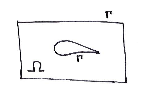
where Γ istheboundaryofthecomputationaldomain Ω (Figure1.1), n istheoutward normalto Γ andtheboundaryflux ˆ F containstheboundaryconditionsdetailedin viscouscaseinsection1.2.2.Weareinterestedbythisunsteadyformulationtogether withthesteadyone,inwhichthetimederivativeisnotintroduced.
Figure1.1. Atypicalcomputationaldomain Ω limited bythetwo-componentboundary Γ= ∂ Ω
1.1.2.2. Discretevariationalrepresentation
Weconsiderherethe steady case,whichiswrittenas
(W )=0 orinvariationalformulation:
Thediscretizationchosenreliesontwomainchoices.First,weconsidera tetrahedrization asthediscretizationofthecomputationaldomain.Thischoiceis madeinconnectionwiththeprogressesmadeforautomaticallygeneratingand adaptingmeshesofthiskind.Second,oncethemeshischosen,wehavetoputonita setofnodesthatarethegeometricalsupportsofthedegreesoffreedom.Theoption chosenisthe setofvertices.Itistheoptionoftheusualcontinuous P 1 FEM
approximation.Itcorrespondstothesmallestnumberofnodesforagivenmesh.Let Th beatetrahedrizationof Ω,whichisadmissibleforfiniteelements,thatis, Ω is partitionedintetrahedra,andtheintersectionoftwodifferenttetrahedraiseither empty,oravertex,oranedge,oraface.Thetestfunctionsaretakenintothe approximationspace Vh madeupofcontinuouspiecewiselinearfunctionsincluded in V =[H 1 (Ω)]5 :
Vh = φh φh iscontinuousand φh |T islinear ∀T ∈Th 5
Inordertoavoidthemanagementofprojectorsapplicableinthewhole H 1 space, weworkinsidethefollowingspaces:
V =([H 2 (Ω)]5 ) and Vh = V ∩ Vh
Itisusefultointroduce Πh thecorresponding P 1 interpolationoperator:
Πh : Vh −→ Vh
Πh φ with Πh φ(i)= φ(i) ∀i vertexof Th .
Thenthediscretesteadyformulationofproblem[1.5]iswrittenas
where Fh isbydefinitionthe P 1 interpolateof F inthesensethat
and,astheoperator Fh appliestothevaluesof W atthemeshvertices,wehave
Wegetthesamerelationsfor ˆ Fh (W ):
Practically,thisdefinitionmeansthatnodalfluxvaluesarewrittenas Fh (xi )= Fh (W (xi )),wherefluxes Fh areevaluatedatthemeshvertices i.Discrete fluxesfunctions x →Fh (x) arederivedfromthenodalvaluesby P 1 intrapolation insideeveryelement.IncontrasttothestandardGalerkinapproach,thisdefinition emphasizesthatthediscretefluxesarein Vh
1.1.2.3.
MEVbasicequivalence
Thediscreteformulation[1.6]canbetransformedintoa vertex-centered finite-volumescheme appliedtotetrahedralunstructuredmeshes.Thisassumesa particularpartitionincontrolcells Ci ofthediscretizeddomain Ωh :
eachcontrolcellbeingassociatedwithavertex i ofthemesh.Thecorrespondingtest functionsarethepiecewiseconstantcharacteristicfunctionsofcells:
χ i (x)= 1 if x ∈ Ci , 0 otherwise.
Then,usingtheStokesformula,thefinite-volumeweakformulation(steadycase) becomesforeachvertex i,thatis,foreachcell Ci ,
where ni holdsfortheunitnormalto ∂Ci outpointingfrom Ci .
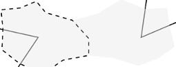
D EFINITION 1.1.– Mediancell:The dualfinite-volumecell isbuiltbytheruleof medians.In2D,themediancellislimitedbysegmentsofmediansbetweencentroids andmid-edge(Figure1.2).In3D,eachtetrahedron T ofthemeshissplitintofour hexahedra2 constructedaroundeachofitsfourvertices.Foravertex i,thehexahedron Ci ∩ T isdefinedbythefollowingpoints(Figure1.3): i)thethreemiddlepointsoftheedgesissuedfrom i; ii)thethreegravitycentersofthefacescontaining i; iii)thecenterofgravityofthetetrahedron; iv)thevertex i
2Thequadrilateralbetweenamidedge,thetwoneighboringfacecentroidsandtetrahedron’s centroidbeingonaplane.
Figure1.2. Illustrationoffinite-volumecellconstructionintwodimensionswithtwo neighboringcells, Ci and Cj ,around i (Pi inthefigure)and j (Pj inthefigure), respectively,andoftheupwindtriangles Kij and Kji associatedwiththeedge ij Representationofthecommonboundary ∂Cij withthesolutionextrapolatedvaluesfor theMUSCLtypeapproach.Dashlinesaresegmentsofmediansofthetriangles
Figure1.3. Theplaneswhichdelimitthefinite-volumecell(relatedto uppervertex)insideatetrahedron(3Dcase). G isthetetrahedron centroid, gk sarefacecentroidsand Ik sareedgecenters
Thecell Ci ofvertex i isthecollectionofallhexahedralinkedto i.Thecommon boundary ∂Cij = ∂Ci ∩ ∂Cj betweentwoneighboringcell Ci and Cj isdividedinto severaltriangularinterfacefacets. ✷
AnillustrationofthisconstructionisshowninFigure1.4forthe3Dcase.
Figure1.4. Illustrationoffinite-volumecellinterface ∂Cij between twoneighboringcells Ci and Cj (3Dcase)
Thefinite-volumefluxesbetweencellsaroundvertices i and j areintegrated throughthecommonboundary ∂Cij withavalueof Fh equaltothehalf-sumof Fh (Wi ) and Fh (Wj ):
where νij denotestheintegralofthenormal ni tocommonboundarybetweencells Ci and Cj ,
νij = ∂Cij ni dσ
and Wi = W (i).Thefinite-volumeformulationforaninternalvertex i writesasthe sumofallthefluxesevaluatedfromthevertices j belongingto V (i) where V (i) is thesetofallneighboringverticesof i.Takingintoaccounttheboundaryfluxes,the discretescheme[1.6]thenwrites:
Weobtainavertex-centeredfinite-volumeapproximation,whichis P 1 -exactwith respecttothefluxfunction Fh .Thisschemeenjoysmostoftheaccuracyproperties
oftheGalerkinmethod(Mer1998),suchasthesecond-orderaccuracyonanymesh fordiffusion-convectionmodels.However,itlacksstabilityandcannotbeappliedto purelyhyperbolicmodelssuchastheEulerequations.
1.1.2.4. Fluxintegration
Oncethecellsaredefined,thespatialdivergence div F istransformedviathe Stokesformulaintointegralsofnormalfluxes F .n atcellboundaries.Inthe proposedfamilyofschemes,theaccuracyoftheintegrationquadratureoncell boundariesisnotascrucial:wechooseaverysimpleoption,the edge-based integration.Onthecontrary,fluxintegrationsetstheimportantproblemofscheme stabilization.Thevariablesareassumedtobeconstantbycell,andtherefore,theyare discontinuousfromacelltoitsneighbor.Upwindintegrationwillrelyonthe Godunovmethodbasedonthetwodifferentvaluesateachsideofthediscontinuity.
1.1.2.4.1.Centraldifferencing
Letuswriteavertex-centeredcentraldifferencedfinite-volumeschemeforthe steadyEulerequationsappliedtoanunstructuredmeshasfollows:
Ψh (Γ,W )i =0, with
h (Γ,W )i = j ∈V (i)
where V (i) isthesetofverticesthatareneighborsof i,and νjk istheintegralon interfacebetween j and k ofthenormalvector.Symbol Bh (Γ,W )i represents boundaryfluxesinwhichEulerfluxestakeintoaccounttheavailableboundary information.Thecenteredintegrationforelementaryflux Φ iswrittenasfollows:
where Fi = F (Wi ) aretheEulerfluxescomputedat Wi .Thisisequivalentto introducethefollowingdiscretespaceoperator ∇∗ h :
where a(i) isthemeasureofcell Ci .
1.1.2.4.2.Godunovdifferencing
Godunov-typemethodsrelyonthediscontinuousrepresentationoftheunknowns atcellinterfacesandonthecomputationofthefluxesatthesediscontinuitiesin
functionofboth“left”and“right”valuesthroughtheapplicationofanapproximate oranexactRiemannsolver.Thisprocessintroducesnumericalviscositytermsthat areveryusefulforstabilizingmostflowcalculations.First,weconsiderthat W is constantbycellequalto Wi in Ci 3.Wewriteavertex-centeredfirst-orderGodunov schemefortheEulerequationsappliedtoanunstructuredmeshasfollows:
Here, ΦARS (Wi ,Wj ,νij ) isevaluatedbyanapproximateRiemannsolver.
RoeapproximateRiemannsolver.AstandardoptionistheRoefluxdifference splitting(Roe1981):
where |A| istheabsolutevalueoftheJacobianfluxalong νij :
3 (
ij )3 (3Dcase) A = T ΛT 1 , Λ= diagonaleigenvaluesmatrix, |A| = T |Λ|T 1 [1.19]
Thesematricesarecomputedatanintermediatevalue W ij of Wi and Wj ;inshort, wehave: W ij =(ρ 1
whichenjoysthefollowingproperty:
F (Wi ) −F (Wj )= A(W ij )(Wi Wj ).
Inthefullysupersoniccaseswhere A(W ij )= |A(W ij )| or A(W ij )= −|A(W ij )|,Roe’ssplittingisfullyupwind.Bythehyperbolicity
3IntheMUSCLmethod,weconsiderthatthemeanvalueincell Ci isidenticaltothevalueat vertex i,anapproximationbringingsimplificationbutnotpermittingtheextensiontoveryhigh order.
assumption,matrix A(W ij ) canbediagonalized.Theabsolutevalue |A(W ij )| is givenas:
where sign(A)= TDiag
Thus,thisaveragingalsopermitsthefollowingequivalentformulation:
HLLCapproximateRiemannsolver.TheideaoftheHLLC4 solver(followingToro 1999)istoconsiderlocallyasimplifiedRiemannproblemwithtwointermediatestates dependingonthelocalleftandrightstates.ThesimplifiedsolutiontotheRiemann problemconsistsofacontactwavewithavelocity SM andtwoacousticwaves,which maybeeithershocksorexpansionfans.Theacousticwaveshavethesmallestand thelargestvelocities(Si and Sj ,respectively)ofallthewavespresentintheexact solution.If Si > 0,thentheflowissupersonicfromlefttorightandtheupwindflux issimplydefinedfrom F (Wi ) where Wi isthestatetotheleftofthediscontinuity. Similarly,if Sj < 0,thentheflowissupersonicfromrighttoleftandthefluxis definedfrom F (Wj ) where Wj isthestatetotherightofthediscontinuity.Inthe moredifficultsubsoniccasewhen Si < 0 <Sj ,wehavetocalculate F (Wi ) or F (Wj ).Consequently,theHLLCfluxisgivenby:
(Wj )
. [1.21] where Wi and Wj areevaluatedasfollows.Letusdenote η = u · n.Assumingthat η = ηi = ηj = SM ,thefollowingevaluationsareproposed(Battenetal.1997)(the subscripts i and j areomittedforclarity):
= 1 S SM
ij
(Wj ) · nij
(S η )
u (S η )+(p p)
4FromHartenetal.(1983)forcontactdiscontinuities.
SM ≤ 0 ≤ Sj
Sj <
Akeyfeatureofthissolverisinthedefinitionofthethreewavesvelocity.Forthe contactwave,weconsider:
andtheacousticwavespeedsbasedontheRoeaverage(denotedby ):
Withsuchwavesvelocities,theapproximateHLLCRiemannsolverhasthe followingproperties(Toro1999):itautomatically(i)satisfiestheentropyinequality, (ii)resolvesisolatedcontactsexactly,(iii)resolvesisolatedshocksexactlyand(iv) preservespositivityof ρ,T,p.
1.1.3. Spatialsecond-orderaccuracy:MUSCL
TheaboveschemeswithRoeorHLLCarespatiallyfirst-orderaccurate. First-orderupwindschemesofGodunovtypeenjoyalotofinterestingqualities,and inparticularHLLCenjoysformallymonotonicityor,inthecaseoftheEulermodel ρ-, T -and p-positivity.Theycanbeextendedtosecondorderbyapplyingthe MUSCLmethod.Indeed,thefactthattheGodunovmethodbuildsfluxesbetween cellswithunknownvariablesconstantbycellsimpliesfirst-orderaccuracy.vanLeer (1979,1977)proposedtoreconstructalinearinterpolationofthevariablesinside eachcellandthentointroduceintheRiemannsolvertheboundaryvaluesofthese interpolations.Further,theslopesusedforlinearreconstructioncanbelimitedin ordertorepresentthevariablewithoutintroducingnewextrema.Theresulting MUSCLmethodproducespositivesecond-orderschemes.Wedescribenowan extensionofMUSCLtounstructuredtriangulationswithdualcells.TheMUSCL ideasalsoapplytoreconstructionswhicharedifferentoneachinterfacebetween cells,orequivalentlyoneachedge.Severalslopesofadependantvariable F are definedonthetwovertices i and j ofanedge ij asfollows:
1) Gradients.First,the centeredgradient (∇F )c ij isdefinedas (∇F )c ij · ij = Fj Fi .
Weconsideracoupleoftwotriangles inm and jrs (2D)ortwotetrahedra inmo and jrst (3D),onehaving i asavertexandthesecondhaving j asavertex.With referencetoFigure1.5,wedefine in , im and io (respectively, jr , js and jt )asthe
componentsofvector ji (respectively, ij )intheobliquesystemofaxes (in, im, io) (respectively, (jr, js, jt)):
ji = in in + im im, + io io,
ij = jr jr + js js + js js.
Figure1.5. Butterflymoleculein2D:localizationoftheextrainterpolation points D ∗ ij and D ∗ ji ofnodalgradients.Thisallowstoevaluatethreederivatives alongdirection ij = Si Sj ,namelywith D ∗ ij and Si ,or Si and Sj ,or Sj and D ∗ ji
Wesaythat Tij and Tji areupwindanddownwindelementswithrespecttoedge ij ifthecomponents in , im , io , jr , js , jt , areallnon-negative: Tij upstreamand Tji downstream ⇔ Min( in , im , io , jr , js , jt ) ≥ 0. [1.22]
The upwindgradient (∇W )u ij iscomputedastheusualfinite-elementgradienton Tij andthe downwindgradient (∇W )d ij on Tji .Thisiswrittenas: (∇W )u ij = ∇W |Tij and (∇W )d ij = ∇W |Tji where ∇W |T = k ∈T Wk ∇Φk |T aretheP1-Galerkingradientsontriangle T .
2) Interpolationatcellinterface.Wenowspecifyourmethodforcomputingthe interpolationslopes (∇ W )ij and (∇ W )ji : (∇W )ij ij =(1 β )(∇W )c ij ij + β (∇W )u ij ij. [1.23]
Thecomputationof Wji isanalogous:
Thecoefficient β isanupwindingparameterthatcontrolsthecombinationoffully upwindandcenteredslopesandthatisgenerallytakenequalto 1/3,accordingtothe erroranalysisinTable1.1. Scheme
RK4(0.11,0.2766,0.5,1)
RK6(Abalakinetal.2002a) 1/3 -1/30 -2/15 5 1.867
RK3-SSP 1/3 0 0 3 2
Table1.1. SuperconvergentordersandmaximalCourantnumbersfor MUSCL-third-order(ξ c = ξ d =0)andV6spatialschemes(1Danalysis).The RK4firstandsecondcoefficientsareoptimizedforhigherCFLwithMUSCL
Figure1.6. Butterflymoleculein3D:downwindandupwindtetrahedra aretetrahedrahaving,respectively, Si and Sj asavertexand suchthatline Si Sj intersectstheoppositeface
3) Fluxbalance.Theschemedescriptioniscompletedbyreplacingthefirst-order formulation[1.17]bythefollowingfluxbalance: