Time–Frequency Analysis of Seismic Signals
Yanghua Wang
Imperial College London
This edition first published © John Wiley & Sons Ltd
All rights reserved. No part of this publication may be reproduced, stored in a retrieval system, or transmitted, in any form or by any means, electronic, mechanical, photocopying, recording or otherwise, except as permitted by law. Advice on how to obtain permission to reuse material from this title is available at http://www wiley com/go/permissions
The right of Yanghua Wang to be identified as the author of the work has been asserted in accordance with law.
Registered Offices
John Wiley & Sons, Inc., 111 River Street, Hoboken, NJ 07030, USA
John Wiley & Sons Ltd, The Atrium, Southern Gate, Chichester, West Sussex, PO19 8SQ, UK
Editorial Office
The Atrium, Southern Gate, Chichester PO19 8SQ, UK
For details of our global editorial offices, customer services, and more information about Wiley products visit us at www.wiley.com
Wiley also publishes its books in a variety of electronic formats and by print-on-demand. Some content that appears in standard print versions of this book may not be available in other formats.
Limit of Liability/Disclaimer of Warranty
The contents of this work are intended to further general scientific research, understanding, and discussion only and are not intended and should not be relied upon as recommending or promoting scientific method, diagnosis, or treatment by physicians for any particular patient. In view of ongoing research, equipment modifications, changes in governmental regulations, and the constant flow of information relating to the use of medicines, equipment, and devices, the reader is urged to review and evaluate the information provided in the package insert or instructions for each medicine, equipment, or device for, among other things, any changes in the instructions or indication of usage and for added warnings and precautions. While the publisher and authors have used their best efforts in preparing this work, they make no representations or warranties with respect to the accuracy or completeness of the contents of this work and specifically disclaim all warranties, including without limitation any implied warranties of merchantability or fitness for a particular purpose. No warranty may be created or extended by sales representatives, written sales materials or promotional statements for this work. The fact that an organization, website, or product is referred to in this work as a citation and/or potential source of further information does not mean that the publisher and authors endorse the information or services the organization, website, or product may provide or recommendations it may make. This work is sold with the understanding that the publisher is not engaged in rendering professional services. The advice and strategies contained herein may not be suitable for your situation. You should consult with a specialist where appropriate. Further, readers should be aware that websites listed in this work may have changed or disappeared between when this work was written and when it is read. Neither the publisher nor authors shall be liable for any loss of profit or any other commercial damages, including but not limited to special, incidental, consequential, or other damages.
Library of Congress Cataloging-in-Publication Data
[HB ISBN: 9781119892342]
Cover Design: Wiley
Cover Image: Courtesy of Yanghua Wang
Set in 10 pt MeridienLTStd by Straive, Chennai, India / 4 1 2023 2023 applied for
This book is dedicated to my wife, Guo-ling, and my two children, Brian and Claire.
3.1
4.6
4.7
5.1
5.3 Implementation of Nonstationary Convolution
5.4 The Inverse W Transform
5.5 Application to Detecting Hydrocarbon Reservoirs
5.6 Application to Detecting Karst Voids
6 The Wigner–Ville Distribution
6.1 Basics of the Wigner–Ville Distribution (WVD)
6.2 Defining the WVD with an Analytic Signal
6.3 Properties of the WVD
6.4 The Smoothed WVD
6.5 The Generalised Class of Time–Frequency Representations
6.6 The Ambiguity Function and the Generalised WVD
6.7 Implementation of the Standard and Smoothed WVDs
6.8 Implementation of the Ambiguity Function and the Generalised WVD
7 Matching Pursuit
7.1 Basics of Matching Pursuit
7.2 Three-stage Matching Pursuit
7.3 Matching Pursuit with the Morlet Wavelet
7.4 The Sigma Filter
7.5 Multichannel Matching Pursuit
7.6 Structure-adaptive Matching Pursuit
7.7 Three Applications
8 Local Power Spectra with Multiple Windows
8.1 Multiple Orthogonal Windows
8.2 Multiple Windows Defined by the Prolate Spheroidal Wavefunctions
8.3 Multiple Windows Constructed by Solving a Discretised Eigenvalue Problem
8.4 Multiple Windows Constructed by Gaussian Functions
8.5 The Gabor Transform with Multiple Windows
8.6 The WVD with Multiple Windows
8.7 Prospective of Time–Frequency Analysis without Windowing
A The Gaussian Integrals, the Gamma Function, and the Gaussian Error Functions
B Fourier Transforms of the Tapered Boxcar Window, the Truncated Gaussian Window, and the Weighted Cosine Window 200
C The Generalised Seismic Wavelet in the Time Domain 203
D Implementation of the Fractional Fourier Transform 205
E Marginal Properties and the Analytic Signal in the WVD Definition 206
F The Prolate Spheroidal Wavefunctions, the Associated and the Ordinary Legendre Polynomials
Preface
The aim of this book, Time–Frequency Analysis of Seismic Signals, is to reveal the local properties of nonstationary seismic signals. Their local properties, such as time period, frequency, and spectral content, vary with time, and the time of seismic signals is a proxy for geologic depth.
Time–frequency analysis is a generalisation of classical Fourier spectral analysis for stationary signals, by extending it to spectral analysis of nonstationary signals. All methods of time–frequency analysis can be treated as a series of implementations of the classical Fourier transform. The kernel of each Fourier transform is formed from a segment of the original seismic signal. Therefore, the time–frequency spectrum is composed of the Fourier spectra generated at different time positions, where the time position corresponds to the centre of each segment.
Different methods of time–frequency analysis differ in the construction of the local kernel, before the Fourier transform is applied. Because of the differences in the construction of the Fourier transform kernel, the methods of time–frequency analysis in this book are divided into two groups.
The first group of methods are the Gabor transform-type methods, including the Gabor transform itself (Chapter 2), the continuous wavelet transform (Chapter 3), the S transform (Chapter 4), and the W transform (Chapter 5). This group of methods focuses on the properties of the different forms of window functions. The window function, which acts as a convolution operator, is applied to the nonstationary signal in a sliding manner. The windowed signal segment is the local kernel for the Fourier transform.
The second group of methods are the energy density distribution methods, including the Wigner–Ville distribution (WVD) (Chapter 6), the matching pursuit-based WVD (Chapter 7), and the local power spectrum with multiple orthogonal windows (Chapter 8). While the resulting time–frequency representation is the energy density distribution, this second
group of methods focuses on manipulating and reformulating the original signal segment to form a time-varying kernel for the Fourier transform.
An essential difference between these two groups of methods is that the Gabor transform-type methods produce complex spectra in the time–frequency plane, while the energy density distribution methods produce real spectra that do not contain phase information. The Gabor transformtype methods have an inverse transform counterpart to reconstruct the original nonstationary signal, and therefore the time–frequency spectra produced by the Gabor transform-type methods can be used in signal processing. However, the energy density distribution methods cannot recover the original signal because the phase information in the time–frequency plane is missing. Consequently, the time–frequency representation of the energy density distribution methods can only be used as a seismic attribute for geophysical characterisation.
With respect to the collective groupings, this book systematically presents various time–frequency analysis methods, including some techniques that have not yet been published or that the author has been instrumental in developing. In presenting each method, the basic theory and mathematical concepts are summarised, with emphasis on the technical aspects.
As such, this book is a practical guide for geophysicists seeking to produce geophysically meaningful time–frequency spectra, process seismic data with time-dependent operations to faithfully represent nonstationary signals, and use the seismic attributes of time–frequency space for the quantitative characterisation of hydrocarbon reservoirs.
Yanghua Wang 25 July 2022
1 Nonstationary Signals and Spectral Properties
Stationary signals are any idealised signals that have time-independent properties, such as time period, frequency, and spectral content. Seismic signals, however, are nonstationary signals that violate the stationary rule described above. When seismic waves propagate through the anelastic media in the Earth’s subsurface, seismic signals have variable properties that vary with the propagation path and travel time.
A stationary signal can be represented mathematically by a stack of sinusoids, using the Fourier transform. In contrast, a nonstationary signal cannot be properly represented by the Fourier transform because the amplitude and frequency of a sinusoidal representation can change dynamically as a function of travel time. To investigate the local properties of a nonstationary signal, an analytic signal-based analysis method can be used instead.
1.1 Stationary Signals
For seismic signals, an idealised stationary model is a stationary convolution process. The physical meaning of the convolution process is ‘superposition’, which is a fundamental principle in the analysis of seismic signals.
Consider an earth model with a layered structure (Figure 1.1). Each layer has a different acoustic impedance, which is the product of velocity and density. The contrast of this physical property between two layers causes seismic reflections at the interface.
Time–FrequencyAnalysisofSeismicSignals, First Edition. Yanghua Wang. © 2023 John Wiley & Sons Ltd. Published 2023 by John Wiley & Sons Ltd.
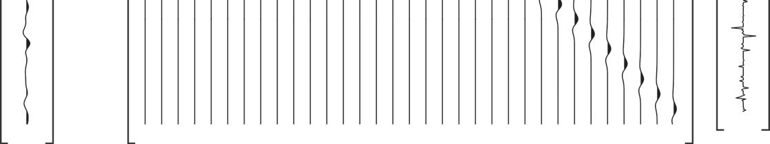
Figure 1.1 The principle of ‘superposition’. Each wavelet is scaled by the reflectivity, which is the contrast in the acoustic impedance between two layers. A seismic trace ()xt is formed by summing all scaled wavelets, which are reflected from various interfaces.
The contrast of acoustic impedance is called reflectivity, or reflection coefficient. The seismic reflectivity includes primary ()pt and multiple (),mt where t is the travel time. The reflectivity series in time consists of both types, ()()(). rtptmt =+ Each reflectivity serves as a scaling factor to scale a particular wavelet ().wt A recorded seismic trace ()xt is formed by summing all scaled wavelets reflected from different interfaces. This physical process is the ‘superposition’ and can be written as
where T [,0121 , , , ] rrrr = r is the vector of the reflectivity series, = w T [,0121 , , , ] n wwww is the vector of the seismic wavelet, and = x T [,0122 , , , ] xxxxn+− is the vector of the seismic trace. If the length of the reflectivity series is , and the length of the seismic wavelet is ,n the length of the resulting seismic trace is 1. n +−
In the superposition process of Eq. (1.1), the wavelet is time shifted and scaled by the reflectivity. Combining all the time-shifted wavelets to form a wavelet matrix, [,0121 , , , ], = Wwwww the superposition process can be expressed in a matrix–vector form, , = xWr and written explicitly as
in which the size of the wavelet matrix W is (1). n +−×
In the matrix–vector form of Eq. (1.2), the wavelet matrix W is a Toeplitz matrix, because each diagonal of W is a constant, ,1,1 ijij++ = WW Then, if we look at the wavelet matrix W row by row, we can see that each row of the matrix consists of the discretised wavelet samples in timereversed order:
Therefore, the matrix–vector form of superposition, , = xWr is the discretised form of ‘convolution’. The corresponding continuous form for the convolution process can be expressed as
where ()wt is the seismic wavelet, ()rt is the subsurface reflectivity series, ∗ is the convolution operator, and ()xt is the seismic trace. In this convolution process, the convolution kernel is the stationary wavelet (),wt which has a constant time period, frequency, and spectral content, with respect to time variation.
A wavelet is a ‘small wave’, for which the time period is relatively short compared to the time duration of the reflectivity series and the resulting seismic trace. With the stationary wavelet (),wt the stationary convolution process of Eq. (1.4) can be depicted as in Figure 1.2.
The stationary wavelet, that is used in Figure 1.2 for the demonstration, is the Ricker wavelet defined as (Ricker, 1953)
where p f is the dominant frequency (in Hz), and 0 t is the central position of the wavelet. The Ricker wavelet is symmetrical with respect to time 0 t and has a zero mean, ()d0.wtt ∞ −∞ = Therefore, it is often known as Mexican hat wavelet in the Americas for its sombrero shape.
Figure 1.2 A stationary convolution process, in which a vector of seismic trace x is generated by the multiplication of a wavelet matrix W and a vector of reflectivity series .r Each column vector of the wavelet matrix W is formed by a stationary seismic wavelet ().wt
1.2 Nonstationary Signals
The stationary convolution process from the previous section is an idealised model for seismic signals. In reality, however, seismic signals are nonstationary due to the dissipation effect when seismic waves propagate through the subsurface anelastic media.
The nonstationary convolution process can be expressed as follows,
where () a wt τ is a nonstationary seismic wavelet, in place of the stationary wavelet ().wt The nonstationary seismic wavelet () a wt τ evolves continually according to a dissipation model:
where ( , ) at τ is the dissipation coefficient, and acts on the idealised stationary wavelet ().wt
In the convolution expression of Eq. (1.7) for the nonstationary wavelet (), a wt τ the dissipation coefficient (,),at τ within which τ indicates the time dependency, is nonstationary. At any given time position , τ the dissipation coefficient ( , ) at τ can be defined by
where i1, =− f is the frequency, ˆ( , ) f ατ is the frequency-dependent attenuation coefficient, and ˆ (,) f β τ is the associated dispersion, i.e. the phase delay of different frequency components (Futterman, 1962).
The attenuation coefficient ˆ( , ) f ατ of seismic waves propagating through the subsurface anelastic media is (Wang & Guo, 2004)
and the associated dispersion ˆ (,) f
τ is
where hf is a reference frequency,
and ()Qt is the quality factor of the subsurface anelastic media (Kolsky, 1956; Futterman, 1962; Wang, 2008). Because seismic signals have a relatively narrow frequency band, it is reasonable to assume ()Qt to be frequency independent. But ()Qt is time dependent, and the time t here is a proxy for geologic depth.
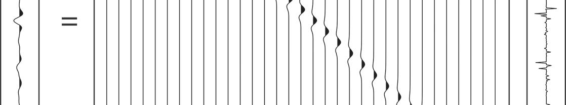
For numerical calculation, the nonstationary convolution process of Eq. (1.6) may also be expressed in a matrix–vector form as
where aW is the nonstationary wavelet matrix. Figure 1.3 depicts this matrix–vector form of the nonstationary convolution process.
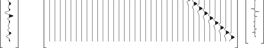
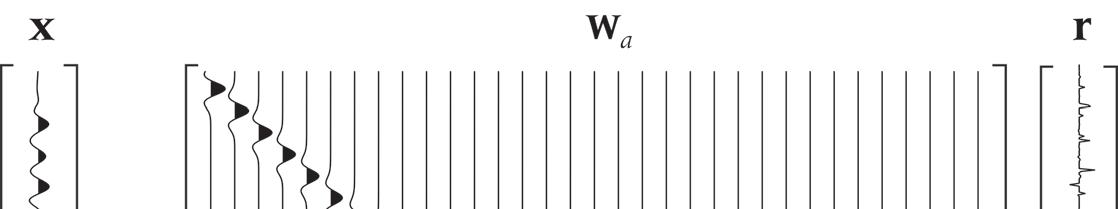
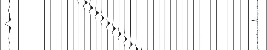
Figure 1.3 The nonstationary convolution process. The wavelet matrix aW is formed by column vectors, each of which is a nonstationary seismic wavelet (), a wt τ and thus the seismic trace ()xt is a nonstationary signal.
The essential distinction between stationary and nonstationary convolution models is the nonstationary wavelet matrix aW While the example symmetrical wavelet in Figure 1.2 is a zero-phase wavelet, the form of the wavelet in Figure 1.3 changes continuously. The amplitude decreases and the phase varies with the travel time. The form of the wavelet gradually changes from symmetrical to asymmetrical.
In general, the differences between stationary and nonstationary signals can be captured in three characteristics.
(1) Time period: The time period for a stationary signal always remains constant, whereas the time period for a nonstationary signal is not constant and varies with time.
(2) Frequency: The frequency of a stationary signal remains constant throughout the process, while the frequency of a nonstationary signal changes continuously during the process.
(3) Spectral content: The spectral content of a stationary signal is constant, while the spectral content of a nonstationary signal varies continuously with respect to time.
For seismic signals, there would be several sets of frequency contents within a given time interval, and these frequency contents are likely to change dynamically with respect to travel time. Therefore, the statistical properties of nonstationary seismic signals also change with time. These statistical properties include the mean, variance, and covariance.
1.3 The Fourier Transform and the Average Properties
The Fourier transform represents a stationary signal as a stack of sinusoids, each of which has a constant frequency and a constant amplitude. Therefore, the Fourier transform is a static spectral analysis that provides only the average characteristics of a nonstationary seismic signal.
For a seismic trace (),xt the Fourier transform is defined as (Bracewell, 1965)
where ˆ()xf is the frequency spectrum of ().xt
The physical meaning of the Fourier transform can be understood by expressing the transform kernel in Euler’s formula,
and rewriting the Fourier transform as follows,
The first integral is a cross-correlation between the seismic signal ()xt and a cosine function, cos(2), ft π and the second integral is a cross-correlation between the seismic signal ()xt and a sine function, sin(2). ft π These two cross-correlations reflect the content of a harmonic component f that is contained in the seismic trace.
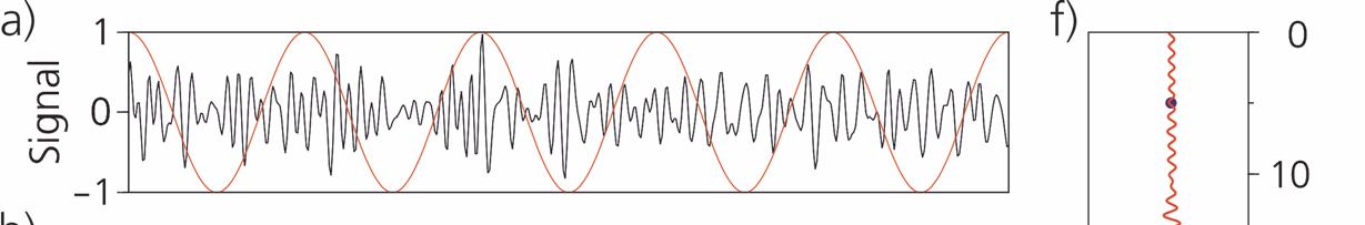
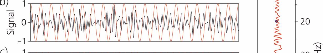
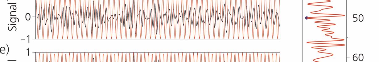
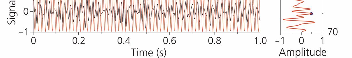
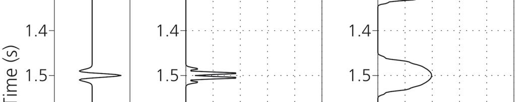
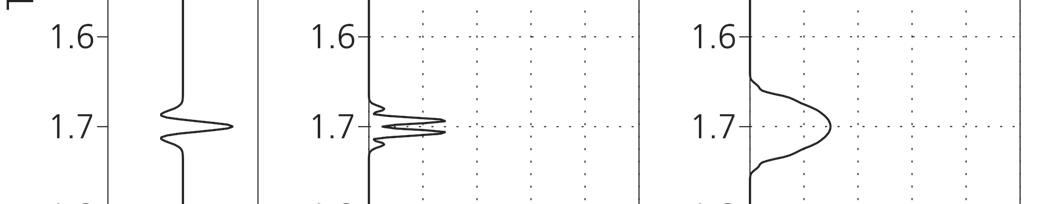
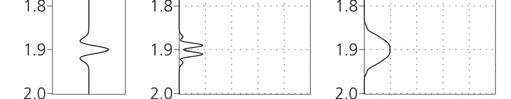
Figure 1.4a−e demonstrate the cross-correlations between a seismic trace and the cosine function at five frequencies of 5, 20, 35, 50, and 65 Hz. The
Figure 1.4 The Fourier transform is the cross-correlation between the seismic trace (black curve) and a cosine function (red curve). (a−e) The cross-correlations at five sample frequencies 5, 20, 35, 50, and 65 Hz. (f) The correlations are marked (solid circles) in the frequency spectrum.
five cross-correlation values are marked in the frequency spectrum that is displayed in the right-hand panel (Figure 1.4f).
The pair of cross-correlations is presented as a complex value, ˆ(),xf which is the frequency spectrum. The cross-correlation with the cosine function is assigned to the real part, ˆ (), R xf and the cross-correlation with the sine function is assigned to the imaginary part, ˆ (). I xf The magnitude of a complex value ˆ()xf is called the amplitude at the given frequency:
The ratio of these two cross-correlations distinguishes their respective weights. Because the ratio of a sine and a cosine function is a tangent function, the inverse function of the ratio is intuitively the phase angle:
Therefore, the frequency spectrum ˆ()xf can be expressed in terms of the amplitude spectrum ˆ()xf and the phase spectrum (), f θ as
The original seismic trace ()xt can be reconstructed precisely from the frequency spectrum ˆ(),xf if the amplitude and phase information of all frequencies of the seismic trace is known. This is the inverse Fourier transform, defined as
The invertibility of the Fourier transform can be easily verified as follows:
One of the important properties of the Fourier transform is energy conservation in both the time and frequency domains (Champeney, 1987):
This is known as Parseval’s theorem, and can be proved thus:
where the superscript ∗ represents a complex conjugate.
According to the definition of the Fourier transform, in which the time integral covers the range of (, ),−∞∞ the frequency spectrum is an average quantity over the entire time duration of a seismic trace.
However, a field seismic trace is composed of signals that travel to and are reflected at different depths, and the signal properties such as amplitude and phase are time dependent. Seismic signals with such time-dependent properties are nonstationary signals.
1.4 The Analytic Signal and the Instantaneous Properties
The classical Fourier transform examines the average properties of a fairly large portion of a seismic trace, but it does not permit the local properties of a nonstationary signal to be examined. The analytic signal analysis method is a transformation method that retains local significance, and the transformation is called the Hilbert transform.
The analytic signal refers to a signal whose spectrum is zero for negative frequencies (Ville, 1948; Ackroyd, 1971). For a real-valued seismic trace
(),xt the Fourier transform ˆ()xf has Hermitian symmetry about the 0 f = axis:
Because of Hermitian symmetry, the negative frequencies are superfluous to the Fourier transform of a real-valued signal ().xt Meanwhile, it seems physically incomprehensible that a real signal has a negative frequency component at all.
The basic idea in building an analytic signal is that such a signal has no negative frequency components:
where ‘sgn’ is the signum function,
The frequency spectrum ˆ()zf contains only the non-negative frequency components of ˆ().xf Then the analytic signal ()zt in the time domain is obtained by the inverse Fourier transform of ˆ():zf
where ()[()] ytxt = is the Hilbert transform of (),xt and ‘p.v.’ denotes the Cauchy principal value (Hilbert, 1912; Hahn, 1996).
According to Eq. (1.26), the analytic signal ()zt is a complex signal, in which the real part ()xt and the imaginary part ()yt are related to each other by the Hilbert transform, which is a time-domain convolution:
limdlimd. (1.27)
The physical meaning of the Hilbert transform is a 2 π ± phase rotation. According to Eq. (1.26), [] 1 ˆ sgn()()i(). fxfyt = Therefore, for the Hilbert transform ()[()], ytxt = the Fourier transform is
Because i2 isgn()e, f π ± −= for 0, f ≠ the Hilbert transform imparts a phase shift of 2 π + to every negative frequency component of the original signal and a phase shift of 2 π to every positive frequency component of the original signal. Because of the 2 π phase offset, ()xt and ()[()] ytxt = are quadrature counterparties.
The analytic signal (),zt that is a complex function of time , t can be written as (Taner etal., 1979)
where ()at is the instantaneous amplitude of the original signal (),xt
and () t θ is the instantaneous phase of the original signal (),xt
In addition to the instantaneous amplitude and the instantaneous phase, another characteristic feature of the nonstationary signal is the instantaneous frequency, which changes constantly with time. According to Eq. (1.29), the instantaneous frequency is the frequency of a sinusoid that best fits the complex signal locally. Therefore, the Fourier transform of ()zt becomes
At time , t the phase is stationary,
This stationary phase condition leads to the definition of the instantaneous frequency:
The physical meaning of the instantaneous frequency (Ackroyd, 1970) can be understood as the centroid of the instantaneous spectrum at time : t
This is a time–frequency spectrum, representing the frequency spectrum of signal ()zt at time t (Ville, 1948).
1.5 Computation of the Instantaneous Frequency
The instantaneous frequency inst ()ft is defined in Eq. (1.34) as the rate of change of the instantaneous phase () t θ However, this definition cannot be used directly to calculate the instantaneous frequency. The arctangent calculation of Eq. (1.31) provides only the principal value of the instantaneous phase (), t θ which must be unwrapped to remove the 2π phase jumps and form a continuous function for the calculation of the instantaneous frequency. Even though, the phase unwrapping process cannot iron out the π ± phase jumps caused by spikes in the noisy seismic trace (Wang, 1998, 2000) and, thus, cannot produce an idealised continuous phase function () t θ for the time differential.
A convenient way of computing the instantaneous frequency inst ()ft is to compute the time differentials, d () d xtt and d () d.ytt Rewriting the arctangent function of Eq. (1.31) as
and differentiating both sides with respect to time , t we have
If 222 ()()()0,atxtyt=+≠ substituting
we obtain the formula of the instantaneous frequency inst (),ft as
Note that, according to the definition of the analytic signal ()zt for a real signal ()xt (Eq. 1.24), the instantaneous frequency must be non-negative, inst ()0.ft ≥
The noisy instantaneous frequency can be further smoothed by a weighted averaging:
where ()Lt is a low-pass filter along the time axis, and ρ is a scaling factor, which is inversely proportional to the size of the low-pass filter. In the averaging formula of Eq. (1.40), the instantaneous amplitude ()at is used as a weighting function to the instantaneous frequency inst ().ft The averaging of the instantaneous frequency inst ()ft over a time window ()Lt ensures that the smoothed frequency inst ()ft is no greater than the Nyquist frequency of a discretised data series (Barnes, 1992).
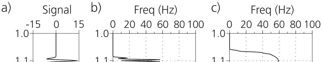
Figure 1.5a shows a synthetic signal, composed of energy-normalised Ricker wavelets, defined as
where p f is the peak frequency. The peak frequencies of the five wavelets are 60, 50, 40, 30, and 20 Hz, respectively. The energy normalisation mimics an idealised situation with no energy attenuation during wave propagation. It can be proved that the energy of this Ricker wavelet (Eq. 1.41) is unity:
Figure 1.5 The concept of the instantaneous frequency. (a) A synthetic trace composed of energy-normalised Ricker wavelets. (b) The instantaneous frequency inst().ft (c) The smoothed instantaneous frequency inst().ft
The proof involves a Gaussian integral (Appendix A):
where n is a positive integer, and () u Γ is the gamma function. In the definition of (), u Γ the real part of variable u is positive, Re()0. u >
Figure 1.5b shows the instantaneous frequency inst ()ft computed through the time differentials of the original signal ()xt and the Hilbert transform ()[()]. ytxt = The computation result contains strong numerical noise.
Figure 1.5c displays the smoothed frequency inst ().ft The low-pass filter ()Lt that is used is a Gaussian function with the Gaussian spread parameter 4,tt σ Δ = where tΔ is the sampling rate in time. Numerical experiments suggest that the scaling factor in Eq. (1.40) can be set as 2 ρ = for the lowpass filter ()Lt with 4.tt σ Δ ≥
Figure 1.6 (a) A two-dimensional seismic profile. (b) The instantaneous frequency profile, which is smoothed in both the time and distance directions.
Figure 1.6 is an example of seismic profile ( , ),xtd and the corresponding profile of instantaneous frequencies inst (,).ftd The instantaneous frequency function is calculated and is smoothed trace by trace. In addition, it is also smoothed along the horizontal direction, by using a Gaussian filter with the spread parameter (2 ), dtdtσσ ΔΔ = where dΔ is the trace interval.
While for nonstationary seismic signals the instantaneous frequency and the instantaneous amplitude can be examined with the analytic signal analysis method described above, the spectral contents, which also vary in time, have to be examined in the time–frequency plane. Therefore, different methods for analysing the time–frequency spectra of nonstationary seismic signals are presented in this book.
1.6 Two Groups of Time–Frequency Analysis Methods
Time–frequency analysis can be considered as a generalisation of the classical Fourier transform of a stationary signal, and applied to the spectral analysis of a nonstationary signal. All methods of time–frequency analysis
can be implemented by the Fourier transform, but they differ in the construction of the transform kernel. Based on the difference in the transformation kernel, I divide the different methods of time–frequency analysis into two groups.
The first group of methods is theGabortransform-typemethod. This group of methods applies various time-window functions to the seismic signal, to form a signal segment, prior to initiating the Fourier transform. In the short-time Fourier transform (STFT), a segment is taken directly from the original signal for the Fourier transform, assuming that the signal segment can be treated as stationary on a short-time basis. The signal segmentation process can be understood as the application of a rectangular window. The application of different time-window functions results in
(1) the Gabor transform (Chapter 2),
(2) the continuous wavelet transform (Chapter 3),
(3) the S transform (Chapter 4), and
(4) the W transform (Chapter 5).
I name this group of methods after Dennis Gabor (1946a, 1946b, 1946c), the pioneer of the STFT method.
The second group of methods is theenergydensitydistributionmethod. The formulation of the transform kernel involves manipulation of the original signal, and the time–frequency representation is the energy density distribution. This group of methods includes
(1) the Wigner–Ville distribution (WVD) (Chapter 6),
(2) the WVD based on the matching pursuit (Chapter 7), and
(3) the local power spectra with multiple windows (Chapter 8).
The kernel in the WVD is the instantaneous autocorrelation of the signal, and not the original signal. The kernel in the WVD based on matching pursuit is the instantaneous autocorrelation of a wavelet, extracted from the original signal by matching pursuit. The local power spectral analysis method manipulates the transform kernel with multiple orthogonal windows. It applies multiple windows in parallel to the same signal segment, and the combined effect of these windows is optimal in retaining the local spectral information of the signal segment.
For the Gabor transform-type method, there are two important features:
(1) The time–frequency spectra produced by the Gabor transform-type method are complex, and the complex spectra consist of both the amplitude spectrum and the phase spectrum.
(2) Consequently, the original signal can be reconstructed by an inverse transform applied to the time–frequency spectrum.
Therefore, the time–frequency spectra can be used in signal processing. If applying a two-dimensional filter to the time–frequency spectrum, the inverse transform produces a filtered signal.
In contrast, two features of the energy density distribution method are:
(1) The energy density distribution in the time–frequency plane is real, and the real spectrum contains no phase information.
(2) Consequently, the original time signal cannot be recovered from the energy density distribution.
The energy density distribution in the time–frequency plane can be used as a seismic attribute for geophysical characterisation.