An Integrative Approach of the Evolution of Living
Coordinated by Eric Guilbert
Apart from any fair dealing for the purposes of research or private study, or criticism or review, as permitted under the Copyright, Designs and Patents Act 1988, this publication may only be reproduced, stored or transmitted, in any form or by any means, with the prior permission in writing of the publishers, or in the case of reprographic reproduction in accordance with the terms and licenses issued by the CLA. Enquiries concerning reproduction outside these terms should be sent to the publishers at the undermentioned address:
ISTE Ltd
John Wiley & Sons, Inc.
27-37 St George’s Road 111 River Street London SW19 4EU Hoboken, NJ 07030
UK USA
www.iste.co.uk
www.wiley.com
© ISTE Ltd 2021
The rights of Eric Guilbert to be identified as the author of this work have been asserted by him in accordance with the Copyright, Designs and Patents Act 1988.
Library of Congress Control Number: 2021941650
British Library Cataloguing-in-Publication Data
A CIP record for this book is available from the British Library
ISBN 978-1-78945-060-6
ERC code:
PE10 Earth System Science
PE10_13 Physical geography
LS8 Ecology, Evolution and Environmental Biology
LS8_1 Ecosystem and community ecology, macroecology
2.1.
2.2.
2.5.
2.6.
2.7.
3.1.
3.2.
3.3.
3.4.
3.5.
3.5.1.
3.5.2.
3.6.
3.7.
4.1.
4.2.
4.2.1.
4.2.2.
4.2.3.
4.2.4.
4.3.
4.3.1.
4.3.2.
4.3.3.
4.4.
4.5.
Julia SCHMACK and Matthew BIDDICK
5.1.
5.2.
5.3. Island biogeography in the Anthropocene
6.1.
6.2.
6.2.1.
6.2.2.
6.3. Vicariance and dispersal shape the global distribution patterns of cave animals
6.3.1. Disjunct distributions and the relictual status of cave biota
6.3.2. Colonization of the subterranean environment: reassessing biogeographic
6.4.
6.5.
6.6.
7.1.
7.2.
7.2.3.
7.3. Soil
7.3.1. The French Monitoring Network of Soil
7.4. Bacterial alpha- and beta-diversity at the national scale
7.4.1. Bacterial alpha-diversity
7.4.2. The bacterial taxa–area relationship
7.5. Spatial distribution and ecological attributes of bacterial taxa at a large scale
7.6. Large-scale bacterial co-occurrence networks (also called Bacteriosociology) ....................................
7.7. Do large-scale bacterial habitats exist?
7.8. Biogeography at the service of environmental
7.9. Conclusion
7.10.
8.1. Introduction
8.2. Fungal
8.3. Biogeographic patterns
8.3.1. Distance-decay of similarity and species area relationship
8.3.2.
8.3.3. Altitudinal
8.4. Functional and interactional biogeography of
8.4.1. Functional biogeography of
8.4.2. Interactional biogeography of
8.4.3. Interactional biogeography of fungi and animals
8.4.4. Interactional biogeography of fungi and bacteria
8.5. Fungal biogeography under global environmental change
8.6. The role of citizen science in the study of fungal biogeography
8.7.
8.8.
9.3.
9.4.
10.3.3. Compositional
Chapter
Jesús OLIVERO
11.1. Introduction
11.1.1. The need of disease mapping for management and prevention policies
11.1.2. Hypotheses on which biogeography sustains the analysis of infectious diseases ...................................
11.2. Do microbes have their own biogeography?
11.3. Historical biogeography and disease
Disease distribution patterns............................
Disease distribution modeling ...........................
11.5.1. Mechanistic versus empirical modeling
11.5.2. The search for risk factors in time and space
11.5.3. Pathogeography: addressing the multifaceted analysis in disease mapping
Chapter 12. Biogeography and Climate Change
Luisa Maria DIELE-VIEGAS
12.1. Climate change
12.1.1. Drivers of climate change
12.2. Impacts of climate change on biodiversity
Chapter 13. Conservation Biogeography: Our Place in the World ......
Brett R. RIDDLE
13.1. The emergence of conservation biogeography ..................
13.2. Milestones in the development of conservation biogeography .........
13.3. The purview of conservation biogeography: claimed and examined......
13.4.
Preface
Eric GUILBERT
UMR7179 MECADEV, National Museum of Natural History, Paris, France
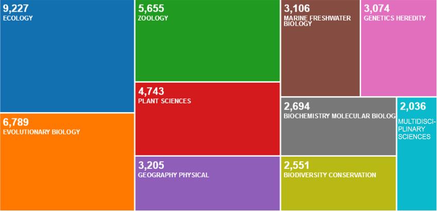
I am pretty sure that most of the scientists working on evolution or the ecology of living organisms did not start as biogeographers … However, when interested in understanding how living organisms have evolved, and how they are organized in relation to their environment, linked to biotic and abiotic variables, biologists naturally arrive at biogeography. Biogeography is the main approach when embracing the history of living species as a whole. It is a huge world, and it is only growing. After a quick search online (Lavoisier.fr), I found 1,291 books on Biogeography written since 1985. Another search, on the Web of Science (wcs.webofknowledge.com), shows 36,567 papers (written between 1957 and 2021) with “biogeography” in the title (Figure P.1). Among these, 25% are associated with “ecology” and 19% with “evolutionary biology”. However, not only ecology and evolutionary biology are linked to biogeography, but a wide range of disciplines, from geography (9%) to genetics (8%) or conservation (7%).
This is why biogeography involves a wide variety of different methods. Which do we use for what purpose? The questions in biogeography are very diverse, and thus the approaches used may be very different. In the second overview of biogeography, Dawson et al. (2016) said the most common term in the 521 abstracts of the 7th biennial meeting of the International Biogeographic Society was “distribution”. In terms of space, “region” was the most common and in terms of time, “history” or “historical” was the most common, followed by “future”. The word “species” was mentioned in 85% of the abstracts. Biogeography still remains the study of the distribution of species in space and time, despite a widening range
Biogeography, coordinated by Eric GUILBERT © ISTE Ltd 2021.
of topics. The future of species is one of the major interests, with the history of species distribution.
Figure P.1. Representation of the number of publications according to different keywords. Source: Web of Science (wcs.webofknowledge.com), March 19, 2021
If terrestrial plant distribution is the main historical beginning of biogeography studies, with the Essai sur la géographie des plantes, written by von Humboldt and Bonpland (1805), the concept was quickly broadened to include other living organisms; see Wallace’s The Geographical Distribution of Animals (1876). After that, progress in taxonomy, systematics and phylogenetics made these studies even broader. New techniques, such as DNA sequencing, ecological niche modeling and many others, have allowed biogeographical approaches to be widened. Dealing with the distribution of Nothofagus (the iconic Southern beech) is not the same as dealing with the propagation of the Ebola virus. Nothofagus has been a key group in biogeographical studies on plants for over 170 years (Cook and Crisp 2005). Despite a huge amount of literature on the subject, the evolution of Nothofagus remains controversial (Hill et al. 2015). On the other hand, the Ebola virus was totally unknown before the 1970s (Pourrut et al. 2005) and, today, drivers that shape the epidemic are much better known, thanks to improvements in approaches and methods (see Chapter 12).
Not only do approaches differ according to the biology of organisms but they also differ according to the environment. Dealing with the biogeography of freshwater fish is not the same as dealing with the biogeography of marine fish. If freshwater habitats can be considered as islands of water in the middle of the land (see Chapter 8), oceans are much less fragmented and more stable environments (see
Chapter 9). How should bacterial distribution in the soil be considered? Drivers of community assemblages of bacteria are specific (Fierer et al. 2007). In addition, taxonomic recognition of bacteria involves molecular tools (see Chapter 7). Is the biogeography of water beetles studied in the same way as the biogeography of cave beetles? The drivers of their distribution may not be the same (see, for example, Arribas et al. 2012; Faille et al. 2014), even if both can be considered as in an insular environment.
A lot of very good books on biogeography have been edited; see, for example, the fifth edition of Biogeography (Lomolino et al. 2017), or Conservation Biogeography (Ladle et al. 2011). Most provide the very bases of biogeography, theories and methods, a wide range of approaches, historical and original cases with nice illustrations. And yet, new studies and methodological novelties are coming out every year, and the number and variety make biogeography so attractive and exciting!
In this book, we have chosen to present an overview of biogeography through different specialists, disciplines, particular living groups or ecosystems and challenging topics, trying to cover a wide range of the current studies in such a broad and multidisciplinary science. The biogeography of terrestrial plants and animals is the very basis of the discipline, yet many topics in these two groups remain unstudied. Many books already cover biogeographical studies on plants and animals and these will not be considered in this book.
After a particular overview of the history of biogeography in Chapter 1, in Chapter 2 we will have an intensive study of the challenges and perspectives of the main analytical approaches used in biogeography, an always-changing world. We will then investigate different approaches, such as phylogeography, dealing with the geographical distribution in gene lineages within species or between closely related species (Chapter 3). Another approach we will look at, in Chapter 4, is geophysical, where the geology and climate conditions are put before biotic processes. We will study different ecosystems, such as islands, in Chapter 5. Since MacArthur and Wilson (1967), how can we miss the famous case of island biogeography! Caves (Chapter 6) are also an extreme ecosystem where species develop specific adaptive skills. Soil bacteria (Chapter 7) is almost an unknown world, a world in which much is still to be done in terms of biogeography, and it deserves a specific approach. In the same way, fungi play an essential role in ecosystem processes, and remain largely unstudied. In Chapter 8, we will also explore the biogeography of fungi, reacting differently according to environmental conditions. In Chapters 9 and 10, we will deal with two different environments, that of freshwater biogeography (Chapter 9) and that of marine biogeography (Chapter 10). One is like islands of
water in the land, while the other is open areas, where terrestrial approaches are not always applicable. Finally, we will focus on particular approaches that are challenging today and may be of greater importance in the future, such as the biogeography of diseases (Chapter 11), a very current field of research, climate change (Chapter 12) and conservation (Chapter 13), two fields that are also closely linked to the human impact on the distribution of species in space and time.
Biogeography is not only a discipline that has been questioning the evolution of species and ecology since naturalists started exploring the world. Understanding patterns and processes of the distribution of species in space and time may provide solutions to the challenges humanity has faced since the era called the Anthropocene and its consequences, such as the biodiversity crisis and global warming.
July 2021
P.1. References
Arribas, P., Velasco, J., Abellan, P., Sanchez-Fernandez, D., Andujar, C., Calosi, P., Millan, A., Ribera, I., Bilton, D.T. (2012). Dispersal ability rather than ecological tolerance drives differences in range size between lentic and lotic water beetles (Coleoptera: Hydrophilidae). Journal of Biogeography, 39, 984–994.
Cook, L.G. and Crisp, M.D. (2005). Not so ancient: The extant crown group of Nothofagus represents a post-Gondwanan radiation. Proceedings of the Royal Society B: Biological Sciences, 272(1580), 2535–2544.
Dawson, M.N., Axmacher, J.C., Beierkuhnlein, C., Blois, J., Bradley, B.A., Cord, A.F., Dengler, J., He, K.A., Heaney, L.R., Jansson, R., Mahecha, M.D., Myers, C., Nogués-Bravo, D., Papadopoulou, A., Reu, B., Rodríguez-Sánchez, F., Steinbauer, M.J., Stigall, A., Tuanmu, M.-N., Gavin, D.G. (2016). A second horizon scan of biogeography: Golden Ages, Midas touches, and the Red Queen. Frontiers of Biogeography, 8(4), 1–30.
Faille, A., Andújar, C., Fadrique, F., Ribera, I. (2014). Late Miocene origin of a Ibero-Maghrebian clade of ground beetles with multiple colonisations of the subterranean environment. Journal of Biogeography, 41, 1979–1990.
Fierer, N., Bradford, M.A., Jackson, R.B. (2007). Toward an ecological classification of soil bacteria. Ecology, 88(6), 1354–1364.
Hill, R.S., Jordan, G.J., Macphail, M.K. (2015). Why we should retain Nothofagus sensu lato. Australian Systematic Botany, 28(3), 190.
von Humboldt, A. and Bonpland, A. (1805). Essai sur la géographie des plantes ; accompagné d’un tableau physique des régions équinocoxiales. Levrault, Schoell & Co., Paris.
Preface xv
Ladle, R.J. and Whittaker, R.J. (2011). Conservation Biogeography. Wiley-Blackwell Press, Oxford.
Lomolino, M.V., Riddle, B.R., Whittaker, R.J. (2017). Biogeography, 5th edition. Oxford University Press, Sunderland, MA.
MacArthur, R.H. and Wilson, E.O. (1967). The Theory of Island Biogeography. Princeton University Press, Princeton, NJ.
Pourrut, X., Kumulungui, B., Wittmann, T., Moussavou, G., Délicat, A., Yaba, P., Nkoghe, D., González, J.-P., Leroy, E.M. (2005). The natural history of Ebola virus in Africa. Microbes and Invection. 7, 1005–1014.
Wallace, A.R. (1876). The Geographical Distribution of Animals: With a Study of the Relations of Living and Extinct Faunas as Elucidating the Past Changes of the Earth’s Surface. Harper & Brothers, New York, NY.
1.1.
1 Origins of Biogeography: A Personal Perspective
Malte C. EBACH
University of New South Wales and The Australian Museum, Sydney, Australia
Introduction: a history of scientific practice
In the 1810 Preface of his Theory of Colours, Johann Wolfgang von Goethe wrote, “The history of an individual displays his [or her] character, so it may here be well affirmed that the history of science is science itself” (Goethe, cited in Duck and Petry 2016, p. xxxv). What Goethe meant is that the past practices of scientists are instances of scientific practice regardless of age. In other words, scientists do not need historians of science to interpret past scientific practice. Scientific practice, no matter how old, will always remain a part of science.
Where, then, does history fit in? Many historians and philosophers of science discuss scientific ideas rather than practice. The reason is that historians and philosophers of science do not engage in scientific practice and are therefore not always able to interpret what we do due to a lack of training or experience or both. British biologist Peter Medawar discussed this in 1968: “What scientists do has never been the subject of a scientific, that is, ethological inquiry… It is no use looking to scientific ‘papers’, for they not merely conceal but actively misrepresent the reasoning that goes into the work they describe” (Medawar 1968, p. 151).
Can historians and philosophers of science trust what scientists say as opposed to what they do? Understanding what scientists do is perhaps a much better way to
Biogeography, coordinated by Eric GUILBERT © ISTE Ltd 2021.
understand the scientific process, rather than believing what they say. Take the science of systematics or taxonomy as an example. Edgar Anderson noted that it is “difficult to write about the taxonomic method [because] in its broadest aspects it has never been described. Taxonomists are more like artists than like art critics; they practice their trade and don’t discuss it” (Anderson, cited in Haas 1954, p. 65). Indeed. What of biogeographical practice? In the case of taxonomy, the result is a list of diagnostic characteristics, names and photographic plates. In biogeography, the results are usually maps. Maps are representative of classifications and are an ideal starting point to understand the early biogeographic method. Before we look at the 18th and 19th biogeographical practices, it is important to understand what biogeography is and how it may be defined1.
1.1.1.
What is biogeography?
The Oxford English Dictionary defines biogeography as “the branch of biology that deals with the geographical distribution of plants and animals. Also: the characteristics of an area or organism in this respect” (OED 2021). The definition is extremely broad, and present-day biogeographers work on a myriad of topics with very different aims and methods. In this sense, biogeography is multidisciplinary, namely the geographical aspect of any field of study that deals with natural objects, be it animals, plants, bacteria fungi, viruses, humans and abiogenesis. It has even made it into nursing pedagogy. In any case, biogeography is a field of enquiry that is dependent on the questions, aims and methods of a particular field. Ecological biogeography, for instance, endeavors to answer ecological questions using methods in ecology. Biogeography is not an independent science with its own unique methods, aims or goals, and attempts to unify it as an “integrative biogeography” have not been successful. Rather than unifying, integrative biogeography discarded a whole suite of approaches and goals in favor of others. We only need to look at the 18th century origins of plant and animal geographies to see that attempts at unification had posed theoretical as well as methodological problems, leading to a split by the end of the 19th century and an abrupt hiatus by the beginning of the 20th century.
1.2. A history of phyto- and zoogeographical classification
1.2.1. Terminology
The goal of finding a phyto- and zoogeographical classification united 18th and 19th century plant and animal geographies. It is important to note that the term
1. For a detailed account of the history of 18th and 19th century biogeographies, see Ebach (2015).
biogeography only appeared in the latter half of the 19th century; Jordan (1883) coined it in German, and Merriam (1892) in English; however, neither author defined the term. The above OED definition of biogeography may have first appeared in Nelson (1978), 90 years after it was first coined2. Regardless, it would be historically incorrect to use the term biogeography for any theory, aims or methods used by 18th and 19th century plant and animal geographers. The term biogeography gained popularity in the latter half of the 20th century. I will use the terms plant and animal geographies, botanical geography, and phytogeography and zoogeography to suit the parlance of the time.
1.2.2. How classification works
Without a classification, it is impossible to scientifically study any natural object. Organisms not only need names, but they need categories to convey meaning. Finding myself in the middle of the North American forest, my friend warned me from afar, “Watch out for the poison ivy!” I knew what ivy was, but how could you tell normal ivy from poison ivy? He could list a set of characteristics that diagnose poison ivy. I am not a botanist so these characteristics would be meaningless; moreover, I would need to touch the poison ivy in order to identity it. “It looks green!” came the reply. My friend was not a botanist either, so I was to avoid a green type of ivy, which I assumed was of a climbing variety. This basic form of communication is helpful to avoid danger or useful to discriminate an edible berry from the one which is toxic. Communication is an essential part of scientific practice as well as its goal. The first question any taxonomists would ask is “What is this?” followed by “What are its characteristics?” and then “What is it most like?” The same is true when we deal with the distributions of animals and plants. Kangaroos do not come from “over there”. They have a particular place in the world, which is determined through a hierarchical classification:
Earth
Southern Hemisphere
Australia
2. I avoid using the phrase “Father of ”. Coining a term does not justify ownership of the whole field. Herman Jordan and Clinton Hart Merriam used the term only once. Jordan casually refers to the term as though it was already in use, and Merriam uses it to describe his “Bio-geographic map”.
There was also an understanding of a basic classification with the poison ivy:
Plant
Ivy Green
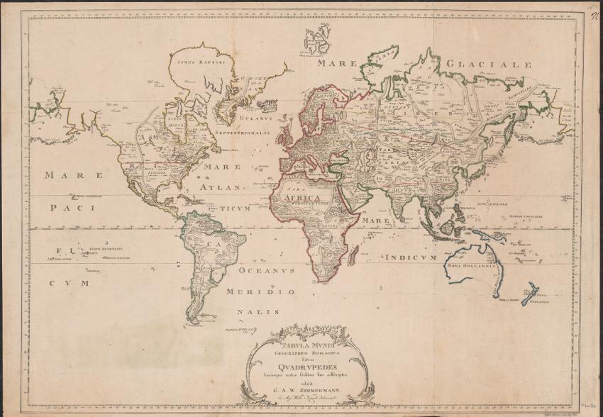
While this is a basic classifications, it works in communicating information and meaning. In order for the classification to work, biogeographers need to be able to communicate plant and animal distributions clearly, either as a list, table or map. A distribution map simply lists where certain organisms occur. Zimmermann (1777) published the first modern distribution map (Figure 1.1) in which the global distributions of terrestrial quadrupeds are named in the areas where they occur. Note that the hierarchy is purely geographical:
Old World
Europe
Africa
Asia
New World
North America
South America
Australasia
Zimmermann’s map was accompanied by a 600-odd page treatise that described the distributions in four chapters:
Chapter I: Animals dispersed throughout the world and their degeneration
Chapter II: Introduction
Part One. Quadrupeds of both the Old and New World
Part the Latter: Quadrupeds of the Old World
Chapter III. Quadrupeds of the New World
Chapter IV. In which the animals are generally treated by the dispersion across the surface, whose consequences are added in the history of the planet (Zimmermann 1777, p. xxiv)
Figure 1.1. Zimmermann’s Tabula mundi geographico zoologica sistems quadrupedes hucusque notos sedibus suis adscriptos, second edition of 1783. Source: National Library of Australia. For a color version of this figure, see www.iste.co.uk/guilbert/biogeography.zip
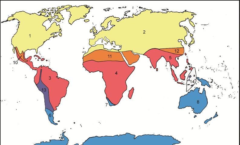
Although Zimmermann’s zoogeographical classification is basic, it does serve a purpose – to explain distribution and dispersal of quadrupeds. Compare the first of these zoogeographical classifications with a more recent bioregionalization by Morrone (2015, Figure 1.2):
Holarctic kingdom
Nearctic region
Palearctic region
Holotropical kingdom
Neotropical region
Ethiopian region
Oriental region
Austral kingdom
Cape region
Andean region
Australian region
Antarctic region
Figure 1.2. The biogeographic regions of Morrone (2015). Areas in yellow are part of the Holarctic kingdom: 1. Nearctic region; 2. Palearctic region. Areas in red are part of the Holotropical kingdom: 3. Neotropical region, 4. Ethiopian region, 5. Oriental region. Areas in blue are part of the Austral kingdom: 6. Andean region 7. Cape region, 8. Australian region, 9. Antarctic region. Areas in orange and purple are transition zones: 10. Mexican, 11. Saharo-Arabian, 12. Chinese, 13. Andean, 14. Indo-Malayan (Wallacea) (Escalante and Morrone 2020, p. 12, Figure 1.2) For a color version of this figure, see www.iste.co.uk/guilbert/biogeography.zip
The areas of Morrone (2015) serve a different purpose, namely to be able to study the relationships of these areas. In fact, Zimmermann’s and Morrone approaches are completely different methodologically, theoretically and historically; yet, both need a classification in order to be able to communicate their ideas to other plant and animal geographers. In other words, it is impossible to do animal and plant geography without a classification. Classifications, however, do not necessarily overlap as in the case of Zimmermann and Morrone. The classification of Zimmermann is based on the geographical regions of the world in the 18th century (note that Antarctica is missing in the former), while that of Morrone has its historical roots in both the zoogeographic Sclater–Wallacean and phytogeographic Humboldtian tradition. But where Zimmermann and Morrone do overlap is that they use the distributions of named species.
One of the many benefits of doing plant and animal geographies, both in the 18th and 21st centuries, is that plant and animal distributions are available in the form of a database. Zimmermann had access to the many travelogues of explorers of his day such as James Cook, Louis Lahontan and Jan Struys, whereas Morrone had access to recent biogeographical classification (i.e. regionalizations) that had used publicly available digital distribution databases such as GBIF. Practically, these two approaches are the same. They are time and cost-effective (neither had to go into the field and collect and describe new species) and they are quick to access (both had access to libraries of one sort or another). Many plant and animal area classifications during the 18th and 19th were collated via the literature (e.g. Stromeyer 1800; Pritchard 1826). But what if you had the funds to go to an area that was poorly understood and under-collected? What if you had the funds to collect plant specimens and other data? How would you classify the natural history of an area? Alexander von Humboldt faced this problem during his journey to New Granada in present-day Colombia during the late 18th century and solved it in a most ingenious way.
1.2.3. Botanical geography versus the geography of plants
The Essai sur la géographie des plantes (Humboldt and Bonpland [1805] 1807) and the 30 volume Le voyage aux régions équinoxiales du Nouveau Continent, fait en 1799, 1800, 1801, 1802, 1803 et 1804 (Humboldt and Bonpland 1814–1829) were the result of a voyage that involved a phenomenal amount of collecting specimens and detailed observations and data collection of astronomical, geological and atmospheric phenomena. In fact, Humboldt amassed enough data to keep himself and Aimé Bonpland occupied until his death in 1859. The problem with collecting a large amount of data is synthesizing it into something useful. The 3,500
species descriptions that would take 15 years to complete was simply too long for someone to make a constructive classification of a fairly unknown area. Humboldt devised something new: a classification based on vegetation. Rather than divide an area based on species distributions, Humboldt used vegetation types, such as “(1) the scitaminales form (Musa, Pothos and Dracontium); (2) the palms; (3) the tree-ferns”, and justifies them:
These divisions based on physiognomy have almost nothing in common with those made by botanists who have hitherto classified them according to very different principles. Only the outlines characterizing the aspect of vegetation and the similarities of impressions are used by the person contemplating nature, whereas descriptive botany [taxonomy] classifies plants according to the resemblance of their smallest but most essential parts […]. The absolute beauty of these shapes, their harmony, and the contrast arising from their being together, all this makes what is called the character of nature in various regions (Humboldt and Bonpland 2009, pp. 73–74).
The notion that plant forms can be used to classify entire regions is central to Humboldtian plant geography. Without needing to know what the species are and to which taxonomic groups they belong, botanists can simply observe overall plant forms in order to classify the vegetation type. Compare this with another attempt at botanical geography using what Humboldt calls “very different principles”.
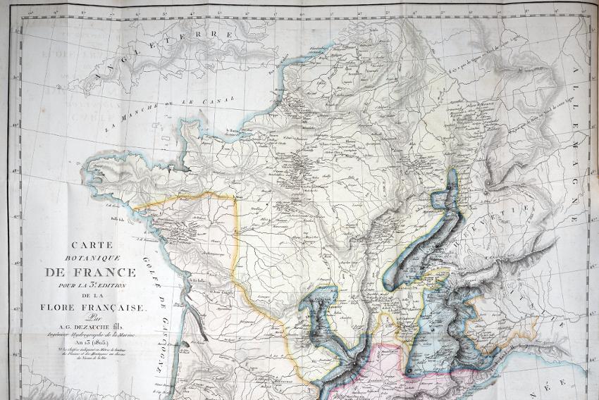
In the same year, Augustin Pyramus de Candolle published the third edition of Flore Française (de Lamarck and de Candolle 1805), which was accompanied by an unusual map (Figure 1.3). The Carte Botanique de la France and a text explaining its function (de Candolle 1805) were “to show the general distribution of plants in France … The map should be considered more of an attempt to apply a specific methodology rather than an attempt to show the complete plant geography of France’’ (de Candolle, cited in Ebach and Goujet 2006, p. 763).
The contrast between Humboldt’s and de Candolle’s attempt is striking. Whereas Humboldt proposes to use plant form, de Candolle opts to use:
1) Temperature, as determined by distance from the equator, height above sea level and southern or northerly exposure.
2) The mode of watering, which is more or less the quantity of water that reaches the plant, the manner by which water is filtered through
the soil and the matter that is dissolved in the water, which may or may not be harmful to the growth of the plant.
3) The degree of soil tenacity or mobility (de Candolle, cited in Ebach and Goujet 2006, p. 768).
Figure 1.3. Carte Botanique de France, pour la 3e Edition de la Flore française par A.G. Dezauche fils Ingénieur Hydrogéologue de la Marine an 13 (1805) “Botanical map of France for the 3rd Edition of Flore française by A.G. Dezauche the son, Marine Hydrological Engineer on the 13th year of the Revolution (1805)” (see Ebach and Goujet 2006, Figure 1.1). For a color version of this figure, see www.iste.co.uk/ guilbert/biogeography.zip
The method proposed by de Candolle did not catch on, and by 1820 de Candolle had chosen to use plant distributions instead, dividing the world into 20 regions:
(1) Boreal Asia, Europe, and America; (2) Europe south of the boreal region and north of the Mediterranean; (3) Siberia; (4) the
Mediterranean area; (5) eastern Europe to the Black and Caspian Seas; (6) India; (7) China, Indochina, and Japan; (8) Australia; (9) south Africa; (10) east Africa; (11) tropical west Africa; (12) Canary Islands; (13) northern United States; (14) northwest coast of North America; (15) the Antilles; (16) Mexico; (17) tropical America; (18) Chile; (19) southern Brazil and Argentina; (20) Tierra del Fuego (de Candolle, cited in Nelson 1978, pp. 283–284).
Again, de Candolle’s plant regions failed to find acceptance. Humboldtian Joakim Frederik Schouw dismissed the regions:
Candolle compares 20 floras, or as he calls them, regions. In his method, which he has developed studying these floras, [Candolle] does not reveal the characteristics that each form takes; it appears that the main basis for the division [of the regions] is current distributions (Schouw 1823, p. 504, my translation).
So too did his son Alphonse de Candolle, who considered “artificial systems”, which are a detriment to science “when they are considered to be natural” (de Candolle 1855, pp. 1304–1305). So what then is a natural region?
The Humboldtians believed that both biotic and abiotic factors, such as climate, were vital in recognizing plant forms and plant regions:
To have an exact acquaintance with these principal forms of vegetation is of the greatest importance to a phyto-geographical division of the globe, as they principally fix the natural physiognomy of different countries. Humboldt is the first who has made such a classification of vegetation, and this must be taken as the foundation of all further inquiry into the subject. It is not until we are somewhat intimately acquainted with the various characteristic forms of plants, that we will be able to recognise the peculiarities of each flora, and to characterise the physiognomy of each country (Meyen 1846, p. 106).
The problem was deciding which abiotic factors were crucial. Schouw had a list of factors that he thought were crucial, so did Heer (1835), Meyen (1846), Sendtner (1854), Lorenz (1863), von Marilaun (1863) and Grisebach (1872). Schouw’s regions all corresponded to climatic zones (e.g. flora Aplino-arctica) and had a dominant vegetation type (e.g. provincia Cichoriacearum), a practice that the Humboldtians used to define areas. Natural areas (and area classifications) were based on the distributions of vegetation that are driven by climate over time, not dissimilar to the concept of biomes of today. Yet by the end of the 19th century,
there was a variety of different area classifications that led Charles Edward Moss to observe that “the subject of ecological plant geography has suffered and still suffers very considerably from a lack of uniformity in the use of its principal terms” (Moss 1910, p. 18).
One idea mentioned by de Candolle (1820) was adopted by the Humboldtians, namely, that of stations and habitations (see Nelson 1978):
By the term station I mean the special nature of the locality in which each species customarily grows; and by the term habitation, a general indication of the country wherein the plant is native. The term station relates essentially to climate, to the terrain of a given place; the term habitation relates to geographical, and even geological, circumstances … The study of stations is, so to speak, botanical topography; the study of habitations, botanical geography … The confusion of these two classes of ideas is one of the causes that have most retarded the science, and that have prevented it from acquiring exactitude” (de Candolle 1820, p. 383, translated in Nelson 1978, p. 280)3
Stations [habitats] and habitations [regions] were the only natural hierarchy that the Humboldtians adopted. The stations were based on physiognomy and the habitations on endemism. Schouw proposed that “at least half the known species are particular [endemic] to a region; 2. that 1/4 of the genera are either fully [endemic] or mostly occur in a region. 3. that single families are either fully [endemic] or mostly occur in a region (Schouw 1823, p. 504, my translation)”. These rules were not that dissimilar to those proposed by de Candolle: “(1) every species tends to occupy a certain space, and the determination of the laws that govern species distributions is the study of habitations; as (2) there are more species in the tropics than in high latitudes; (3) the numbers of species of monocots and dicots vary in certain ways; (4) certain numbers of species are recorded for certain countries” (de Candolle 1820, pp. 392–400 in Nelson 1978, p. 281). In this sense, you preserve both classifications: plant taxonomy is used to identify plants and species; genera and families are used to determine the larger habitations; and plant forms and vegetation are used to classify the smaller stations. In The History of Biology, Nordenskiöld (1936) summed up plant geography as having taken “two courses”, “a systematical, which is ultimately based on Linnæus’s observations and theories in
3. Later, Gareth Nelson was to note that “the concepts of station and habitation are important in Candolle’s view, for they define two different sciences, which persist into the modern era […]. No matter, the terms as used by Candolle, have modern counterparts: ecological and historical biogeography. Ecological biogeography is the study of stations; historical biogeography, the study of habitations” (Nelson 1978, p. 280, footnote 31, 281).
connexion with the distribution of the plant species, and a morphological [physiognomic], which has its origins in Humboldt’s theories on the morphological association of different vegetable types with different countries and forms of landscape”. Of the latter, Nordenskiöd states, “œcological plant geography does not investigate the nature of the flora, but of the vegetation. It works not with species, but with plant communities [populations]” (Nordenskiöld 1936, pp. 560–561). I will return to the plight of plant geography at the start of the 20th century later.
1.2.4. Zoogeography: a search for natural regions
Animal geography had a later start than plant geography. Although Zimmermann (1778–1783) was the first to consider an animal geography, it was confined to quadrupeds. Unlike the Humboldtians and de Candolle, animal geographers rarely looked at faunal regions, instead preferring to look at taxon-specific distributions. Also, a contemporary of Zimmermann, Johan Christian Fabricius, proposed eight climatic regions “from which the Stations of insects are judged” (Fabricius 1778, p. 154). Zoologists did not adopt the Humboldtian tradition of using “form” and dismissed the climatic regions of Fabricius as arbitrary or artificial:
This simple statement is enough to convince us that there is a lot of arbitrariness in these divisions (Latreille 1815, pp. 40–41, my translation).
[Fabricius] … by not attempting to demonstrate the correctness of any one of his divisions, seems to have subsequently abandoned them altogether, since no one, it may be fairly presumed, was more qualified than himself to discover the artificial nature of his theory (Swainson 1835, pp. 10–11).
Similarly, the regions proposed by Pierre André Latreille in 1817, based on latitudinal and longitudinal gradients along climatic zones, were equally dismissed:
Any division of the globe into climates, by means of equivalent parallels and meridians, wears the appearance of an artificial and arbitrary system, rather than to one according to nature (Kirby and Spence 1828, p. 487).
Entomologists William Swainson, William Kirby and William Spence were insistent on the necessity of defining natural regions, namely “those grand divisions of animal geography pointed out by nature, and immediately recognized by every naturalist” (Swainson 1835, p. 11). Swainson places William Sharp Macleay and Humboldt among those who recognize that natural areas are not “regulated by
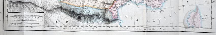
isothermal lines” (Swainson 1835, p. 12). The famous Tableau Physique of Humboldt, depicting mounts Chimborazo and Cotopaxi in the Andes, were drawn in cross-section in order to highlight isothermal lines4 (Figure 1.4). We can imagine that Swainson considered all lines, be they isothermal lines or latitudinal lines, as artificial. Yet, isothermal lines were quite popular with plant and animal geographers in delimiting climatic zones. Given, however, that climate and plant forms define vegetation, we could argue that the Humboldtians would consider such lines to portray natural areas. After all “only those vegetative formations deserve to be recognised as independent plant forms, which conform to the influence of climate” (Grisebach 1866, p. 384).
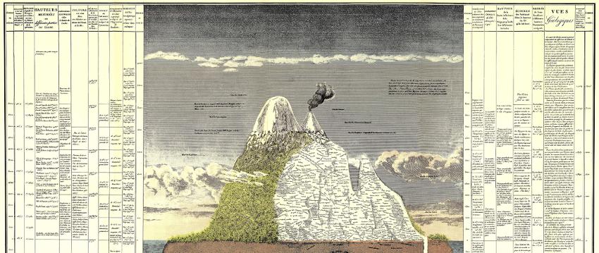

Figure 1.4. Humboldt’s Tableau physique showing a cross-section of Mount Chimborazo and Mount Cotopaxi in the Andes. The full title of the map reads: Geographie des plantes equinoxiales : tableau physique des Andes et Pays voisins. Dressé d’après des observations et des Mesures prises sur les lieux depuis le 10.degré de l’attitude australe en 1799, 1800, 1801, 1802 et 1803 (in Humboldt and Bonpland 1807) (source: http://cybergeo.revues.org/docannexe/image/25478/img-7.jpg). For a color version of this figure, see www.iste.co.uk/guilbert/biogeography.zip
4. The Tableau lacks the actual lines, but instead has a table on either side of the cross-section depicting the temperatures at elevation. Essentially, Humboldt has created a sophisticated isothermal line.
While some zoologists would adopt a more Humboldtian approach to delimiting areas using climate, such as the homoiozoic belts of Forbes (1856) or the life zones of Merrian (1892), others sought to look only at the distribution of species. An earlier attempt at using animal distributions to define animal regions was proposed by Johann Karl Wilhelm Illiger in 1815. Illiger (1815) attempted to summarize the global geographical distribution of mammals by counting the number of species that occurred in each continent. Much of Illiger (1815) are tables listing the names of genera, families and orders and the numbers of species found in each continent. The work is completely taxonomic, devoid of any measurements of temperature or rainfall, and synthetic, as it had collated names of species from the works of others. The body of work is divided into sections or “comparative summaries” based on each of the tables, including a description of the faunal distribution of a list of the taxa. A modern-day biogeographer would be impressed with the volume of data but perplexed with how little Illiger had done with it. German paleontologist Johann Andreas Wagner synthesized Illiger (1815) into four mammalian provinces in a three-part work published between 1844 and 1846 (Wagner 1844–1846). The work also included the first known global biogeographic map (Figure 1.5). Wagner was also the first to use a hierarchical classification of zones, provinces, sub-provinces and regions (Table 1.1). More important, Wagner considered these divisions to be natural. In staying with Illiger’s style of only listing the distributions of mammals, Wagner stands out in zoological and botanical geography by ignoring abiotic factors such as climate. Wagner’s contemporary Ludwig Schmarda’s Distribution of Animals (Schmarda 1853), for example, discusses the influence of climate, water and temperature, as well as denoting “tropical forms” and the interaction with vegetation. Schmarda’s map of the geographical distribution of animals is possibly the most detailed of any zoogeographical study in the 19th century. The map depicts 21 terrestrial and 10 oceanic areas and the distributions of various taxa, as well as the location of reefs, atolls, the direction of ocean currents, isothermal lines and latitude and longitude. Unlike Wagner’s classification, Schmarda’s was non-hierarchical and partially based on climate. Unfortunately, Wagner’s work was largely ignored and those who did notice it never quite fully appreciated its significance. The nearest zoogeographical work to resemble Wagner’s appeared a decade later. Philip Lutley Sclater, who used a similar method to Wagner, namely counting taxa, proposed a hierarchical classification. Sclater, however, offered something new:
In the Physical Atlases lately published, which have deservedly attracted no small share of attention on the part of the public, too little regard appears to have been paid to the fact that the divisions of the earth’s surface usually employed are not always those which we most
natural when their respective Faunæ and Flora are taken into consideration. The world is mapped out into so many portions, according to latitude and longitude, and an attempt is made to give the principal distinguishing characteristics of the Fauna and Flora of each of these divisions; but little or no attention is given to the fact that two or more of these geographical divisions may have much closer relations to each other than to any third, and, due regard being paid to the general aspect of their Zoology and Botany, only form one natural province or kingdom (as it may perhaps be termed), equivalent in value to that third (Sclater 1858, pp. 130–131).
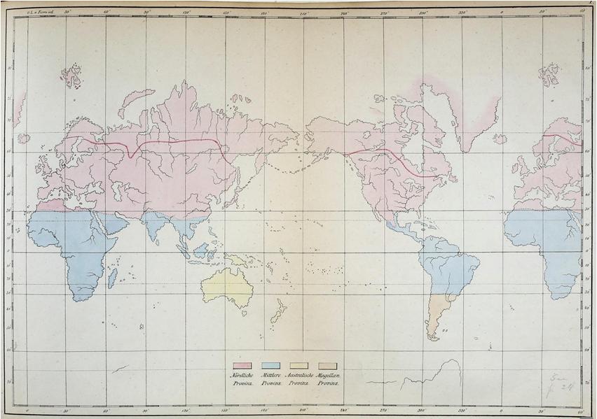
Figure 1.5. “Representation of the distribution of mammals according to their zones and their provinces. The southern boundary of the northern polar province is indicated by a line of a different color, drawn somewhat further south than the equatorial border of the arctic fox ([Vulpes] lagopus), though not so far in some places as the reindeer may descend there on their summer migrations. The southern polar province is not included in this map, because it is only in the process of discovery and, according to all previous experience, it does not harbour land mammals” (Wagner 1844, 241, Table 1.1). For a color version of this figure, see www.iste.co.uk/guilbert/biogeography.zip