Visit to download the full and correct content document: https://ebookmass.com/product/excel-formulas-functions-6th-edition-ken-bluttman/
More products digital (pdf, epub, mobi) instant download maybe you interests ...
Microsoft Excel Formulas and Functions (Office 2021 and Microsoft 365) Paul Mcfedries
https://ebookmass.com/product/microsoft-excel-formulas-andfunctions-office-2021-and-microsoft-365-paul-mcfedries/
Excel 2022 3 Books In 1: A to Z Mastery Guide on Excel Basic Operations, Excel Formulas Joe Webinar
https://ebookmass.com/product/excel-2022-3-books-in-1-a-to-zmastery-guide-on-excel-basic-operations-excel-formulas-joewebinar/
Up Up and Array!: Dynamic Array Formulas for Excel 365 and Beyond 1st Edition Abbott Ira Katz
https://ebookmass.com/product/up-up-and-array-dynamic-arrayformulas-for-excel-365-and-beyond-1st-edition-abbott-ira-katz-2/
Up Up and Array!: Dynamic Array Formulas for Excel 365 and Beyond 1st Edition Abbott Ira Katz
https://ebookmass.com/product/up-up-and-array-dynamic-arrayformulas-for-excel-365-and-beyond-1st-edition-abbott-ira-katz/
Excel VBA Programming For Dummies 6th Edition Dick Kusleika
https://ebookmass.com/product/excel-vba-programming-fordummies-6th-edition-dick-kusleika/
Destination C1 & C2 : grammar & vocabulary with answer key 18 [printing]. Edition Malcolm Mann
https://ebookmass.com/product/destination-c1-c2-grammarvocabulary-with-answer-key-18-printing-edition-malcolm-mann/
Functions and Change: A Modeling Approach to College Algebra
6th Edition Bruce Crauder
https://ebookmass.com/product/functions-and-change-a-modelingapproach-to-college-algebra-6th-edition-bruce-crauder/
Basic Immunology: Functions and Disorders of the Immune System 6th Edition Abul Abbas Mbbs
https://ebookmass.com/product/basic-immunology-functions-anddisorders-of-the-immune-system-6th-edition-abul-abbas-mbbs/
Elsevier Weekblad - Week 26 - 2022 Gebruiker
https://ebookmass.com/product/elsevier-weekbladweek-26-2022-gebruiker/
Excel® Formulas & Functions For Dummies®, 6th Edition
Published by: John Wiley & Sons, Inc., 111 River Street, Hoboken, NJ 07030-5774, www.wiley.com
Copyright © 2022 by John Wiley & Sons, Inc., Hoboken, New Jersey
Published simultaneously in Canada
No part of this publication may be reproduced, stored in a retrieval system or transmitted in any form or by any means, electronic, mechanical, photocopying, recording, scanning or otherwise, except as permitted under Sections 107 or 108 of the 1976 United States Copyright Act, without the prior written permission of the Publisher. Requests to the Publisher for permission should be addressed to the Permissions Department, John Wiley & Sons, Inc., 111 River Street, Hoboken, NJ 07030, (201) 748-6011, fax (201) 748-6008, or online at http://www.wiley.com/go/permissions
Trademarks: Wiley, For Dummies, the Dummies Man logo, Dummies.com, Making Everything Easier, and related trade dress are trademarks or registered trademarks of John Wiley & Sons, Inc. and may not be used without written permission. Microsoft and Excel are trademarks or registered trademarks of Microsoft Corporation. All other trademarks are the property of their respective owners. John Wiley & Sons, Inc. is not associated with any product or vendor mentioned in this book.
LIMIT OF LIABILITY/DISCLAIMER OF WARRANTY: WHILE THE PUBLISHER AND AUTHORS HAVE USED THEIR BEST EFFORTS IN PREPARING THIS WORK, THEY MAKE NO REPRESENTATIONS OR WARRANTIES WITH RESPECT TO THE ACCURACY OR COMPLETENESS OF THE CONTENTS OF THIS WORK AND SPECIFICALLY DISCLAIM ALL WARRANTIES, INCLUDING WITHOUT LIMITATION ANY IMPLIED WARRANTIES OF MERCHANTABILITY OR FITNESS FOR A PARTICULAR PURPOSE. NO WARRANTY MAY BE CREATED OR EXTENDED BY SALES REPRESENTATIVES, WRITTEN SALES MATERIALS OR PROMOTIONAL STATEMENTS FOR THIS WORK. THE FACT THAT AN ORGANIZATION, WEBSITE, OR PRODUCT IS REFERRED TO IN THIS WORK AS A CITATION AND/OR POTENTIAL SOURCE OF FURTHER INFORMATION DOES NOT MEAN THAT THE PUBLISHER AND AUTHORS ENDORSE THE INFORMATION OR SERVICES THE ORGANIZATION, WEBSITE, OR PRODUCT MAY PROVIDE OR RECOMMENDATIONS IT MAY MAKE. THIS WORK IS SOLD WITH THE UNDERSTANDING THAT THE PUBLISHER IS NOT ENGAGED IN RENDERING PROFESSIONAL SERVICES. THE ADVICE AND STRATEGIES CONTAINED HEREIN MAY NOT BE SUITABLE FOR YOUR SITUATION. YOU SHOULD CONSULT WITH A SPECIALIST WHERE APPROPRIATE. FURTHER, READERS SHOULD BE AWARE THAT WEBSITES LISTED IN THIS WORK MAY HAVE CHANGED OR DISAPPEARED BETWEEN WHEN THIS WORK WAS WRITTEN AND WHEN IT IS READ. NEITHER THE PUBLISHER NOR AUTHORS SHALL BE LIABLE FOR ANY LOSS OF PROFIT OR ANY OTHER COMMERCIAL DAMAGES, INCLUDING BUT NOT LIMITED TO SPECIAL, INCIDENTAL, CONSEQUENTIAL, OR OTHER DAMAGES.
For general information on our other products and services, please contact our Customer Care Department within the U.S. at 877-762-2974, outside the U.S. at 317-572-3993, or fax 317-572-4002. For technical support, please visit https://hub.wiley.com/community/support/dummies.
Wiley publishes in a variety of print and electronic formats and by print-on-demand. Some material included with standard print versions of this book may not be included in e-books or in print-on-demand. If this book refers to media such as a CD or DVD that is not included in the version you purchased, you may download this material at http://booksupport.wiley.com. For more information about Wiley products, visit www.wiley.com
Library of Congress Control Number: 2021948499
ISBN 978-1-119-83911-8 (pbk); ISBN 978-1-119-83912-5 (ebk); ISBN 978-1-119-83913-2 (ebk)
Part 2: Doing the Math
Part 3: Solving with Statistics
CHAPTER 9: Throwing
11: Rolling the Dice on Predictions and Probability
Part 4: Dancing with Data
Part 5: The Part of Tens
Getting It Straight: Using SLOPE and INTERCEPT to Describe Linear Data
What’s Ahead: Using FORECAST, TREND, and GROWTH to Make Predictions
Using NORM.DIST and POISSON.DIST to Determine Probabilities
PART 4: DANCING WITH DATA
Formatting
Finding Where the Data Is
Going
Counting
Part of a Year with YEARFRAC
Find the Data TYPE
Find the LENgth of Your Text
Just in CASE
Working with Excel Fundamentals
Before you can write any formulas or crunch any numbers, you have to know where the data goes and how to find it again. I wouldn’t want your data to get lost! Knowing how worksheets store your data and present it is critical to your analysis efforts.
Understanding workbooks and worksheets
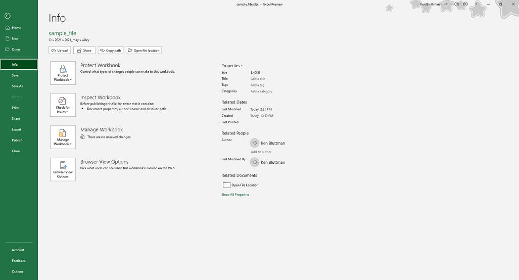
In Excel, a workbook is the same as a file. Excel opens and closes workbooks, just as a word processor program opens and closes documents. When you start up Excel, you are presented with a selection of templates to use, the first one being the standard blank workbook. Also there is a selection of recent files to select from. After you open a new or already created workbook, click the File tab to view basic functions such as opening, saving, printing, and closing your Excel files (not to mention a number of other nifty functions to boot!). Figure 1-1 shows the contents presented on the Info tab.
The default Excel file extension is .xlsx. However you may see files with the older .xls extension. These older files work fine in the latest version of Excel.
Start Excel and double-click the Blank Workbook icon to create a new blank workbook. When you have more than one workbook open, you pick the one you want to work on by clicking it on the Windows Taskbar.
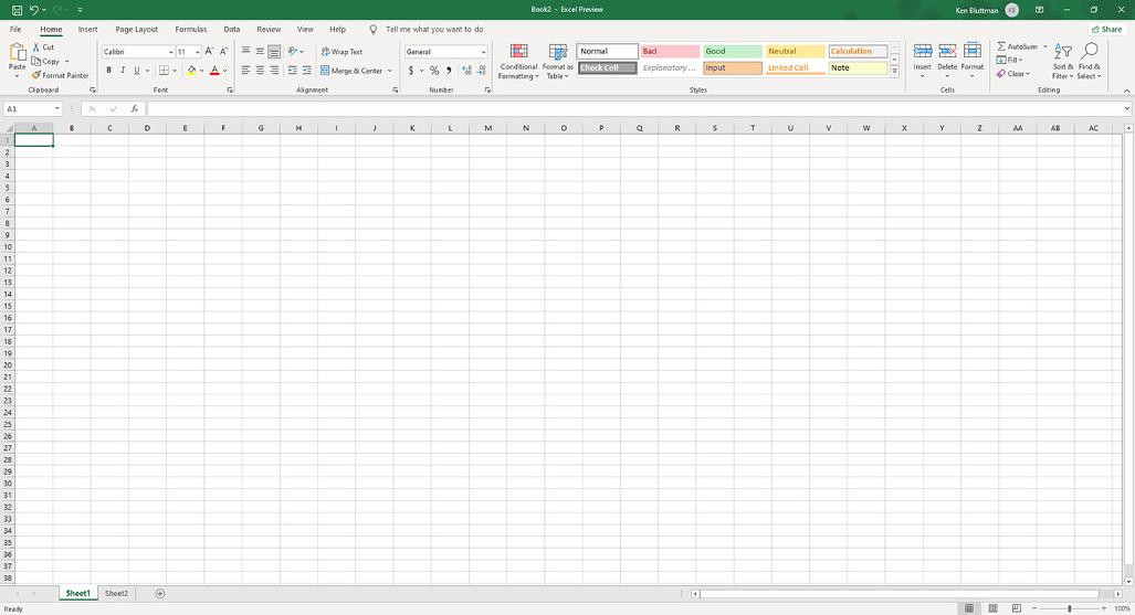
A worksheet is where your data actually goes. A workbook contains at least one worksheet. If you didn’t have at least one, where would you put the data? Figure 1-2 shows an open workbook that has two sheets, aptly named Sheet1 and Sheet2. To the right of these worksheet tabs is the New Sheet button (looks like a plus sign), used to add worksheets to the workbook.
FIGURE 1-1: The Info tab shows details about your Excel file.
FIGURE 1-2: Looking at a workbook and worksheets.
At any given moment, one worksheet is always on top. In Figure 1-2, Sheet1 is on top. Another way of saying this is that Sheet1 is the active worksheet. There is always one and only one active worksheet. To make another worksheet active, just click its tab.
Worksheet, spreadsheet, and just plain old sheet are used interchangeably to mean the worksheet.
What’s really cool is that you can change the name of the worksheets. Names like Sheet1 and Sheet2 are just not exciting. How about Baseball Card Collection or Last Year’s Taxes? Well, actually, Last Year’s Taxes isn’t too exciting, either.
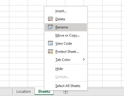
FIGURE 1-3: Changing the name of a worksheet.
The point is, you can give your worksheets meaningful names. You have two ways to do this:
» Double-click the worksheet tab and then type a new name.
» Right-click the worksheet tab, select Rename from the menu, and then type a new name.
Figure 1-3 shows one worksheet name already changed and another about to be changed by right-clicking its tab.
You can try changing a worksheet name on your own. Do it the easy way:
1. Double-click a worksheet’s tab.
2. Type a new name and press Enter. The name cannot exceed 31 characters.
You can change the color of worksheet tabs. Right-click the tab and select Tab Color from the menu. Color coding tabs provides a great way to organize your work.
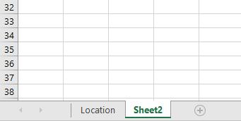
To insert a new worksheet into a workbook, click the New Sheet button, which is located after the last worksheet tab. Figure 1-4 shows how. To delete a worksheet, just right-click the worksheet’s tab and select Delete from the menu.
FIGURE 1-4: Inserting a new worksheet.
Don’t delete a worksheet unless you really mean to. You cannot get it back after it is gone. It does not go into the Windows Recycle Bin.
You can insert many new worksheets. The limit of how many is based on your computer’s memory, but you should have no problem inserting 200 or more. Of course, I hope you have a good reason for having so many, which brings me to the next point.
Worksheets enable you to organize your data. Use them wisely, and you will find it easy to manage your data. For example, say that you are the boss (I thought you’d like that!), and over the course of a year you track information about 30 employees. You may have 30 worksheets — one for each employee. Or you may have 12 worksheets — one for each month. Or you may just keep it all on one worksheet. How you use Excel is up to you, but Excel is ready to handle whatever you throw at it.
You can set how many worksheets a new workbook has as the default. To do this, click the File tab, click Options, and then click the General tab. Under the When Creating New Workbooks section, use the Include This Many Sheets spinner control to select a number.
Introducing the Formulas tab
Without further ado, I present the Formulas tab of the Ribbon. The Ribbon sits at the top of Excel. Items on the Ribbon appear as menu headers along the top of the Excel screen, but they actually work more like tabs. Click them, and no menus appear. Instead, the Ribbon presents the items that are related to the clicked Ribbon tab.
Figure 1-5 shows the top part of the screen, in which the Ribbon displays the items that appear when you click the Formulas tab. In the figure, the Formulas tab is set to show formula-based methods. At the left end of the tab, functions are categorized. One of the categories is opened to show how you can access a particular function.
FIGURE 1-5: Getting to know the Ribbon.
These groups are along the bottom of the Formulas tab:
» Function Library: This includes the Function Wizard, the AutoSum feature, and the categorized functions.
» Defined Names: These features manage named areas, which are cells or ranges on worksheets to which you assign a meaningful name for easy reference.
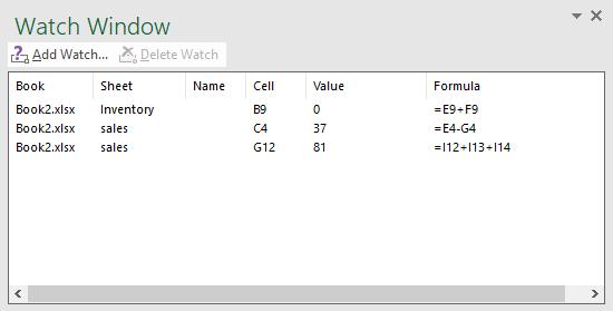
» Formula Auditing: These features are for checking and correcting formulas. Also here is the Watch Window, which lets you keep an eye on the values in designated cells, but within one window. In Figure 1-6 you can see that a few cells have been assigned to the Watch Window. If any values change, you can see this in the Watch Window. Note how the watched cells are on sheets that are not the current active sheet. Neat! By the way, you can move the Watch Window around the screen by clicking the title area of the window and dragging it with the mouse.
» Calculation: This is where you manage calculation settings, such as whether calculation is automatic or manual.
FIGURE 1-6:
Eyeing the Watch Window.
Another great feature that goes hand in hand with the Ribbon is the Quick Access Toolbar. (So there is a toolbar after all!) In Figure 1-5, the Quick Access Toolbar sits just above the left side of the Ribbon. On it are icons that perform actions with a single click. The icons are ones you select by using the Quick Access Toolbar tab in the Excel Options dialog box. You can put the toolbar above or below the Ribbon by clicking the Customize Quick Access Toolbar drop-down arrow on the Quick Access Toolbar and choosing an option. In this area too are the other options for the Quick Access Toolbar.
Working with rows, columns, cells, ranges, and tables
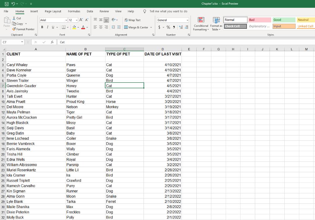
A worksheet contains cells. Lots of them. Billions of them. This might seem unmanageable, but actually it’s pretty straightforward. Figure 1-7 shows a worksheet that contains data. Use this to look at a worksheet’s components. Each cell can contain data or a formula. In Figure 1-7, the cells contain data. Some, or even all, cells could contain formulas, but that’s not the case here.
Columns have letter headers — A, B, C, and so on. You can see these listed horizontally just above the area where the cells are. After you get past the 26th column, a double lettering system is used — AA, AB, and so on. After all the two-letter combinations are used up, a triple-letter scheme is used. Rows are listed vertically down the left side of the screen and use a numbering system.
You find cells at the intersection of rows and columns. Cell A1 is the cell at the intersection of column A and row 1. A1 is the cell’s address. There is always an active cell — that is, a cell in which any entry would go into should you start typing. The active cell has a border around it. Also, the contents of the active cell appear in the Formula Box.
FIGURE 1-7: Looking at what goes into a worksheet.
When I speak of, or reference, a cell, I am referring to its address. The address is the intersection of a column and row. To talk about cell D20 means to talk about the cell that you find at the intersection of column D and row 20.
GETTING TO KNOW THE FORMULA BAR
Taken together, the Formula Box and the Name Box make up the Formula Bar. You use the Formula Bar quite a bit as you work with formulas and functions. The Formula Box is used to enter and edit formulas. The Formula Box is the long entry box that starts in the middle of the bar. When you enter a formula into this box, you can click the little check-mark button to finish the entry. The check-mark button is visible only when you are entering a formula. Pressing Enter also completes your entry; clicking the X cancels the entry.
An alternative is to enter a formula directly into a cell. The Formula Box displays the formula as it is being entered into the cell. When you want to see just the contents of a cell that has a formula, make that cell active and look at its contents in the Formula Box. Cells that have formulas do not normally display the formula, but instead display the result of the formula. When you want to see the actual formula, the Formula Box is the place to do it. The Name Box, on the left side of the Formula Bar, is used to select named areas in the workbook.
FIGURE 1-8: Selecting a range of cells.
In Figure 1-7, the active cell is C7. You have a couple of ways to see this. For starters, cell C7 has a border around it. Also notice that the column head C is shaded, as well as row number 7. Just above the column headers are the Name Box and the Formula Box. The Name Box is all the way to the left and shows the active cell’s address of C7. To the right of the Name Box, the Formula Box shows the contents of cell C7.
If the Formula Bar is not visible, choose File ➪ Options, and click the Advanced tab. Then, in the Display section in the Excel Options dialog box, select the Show Formula Bar check box to make the Formula Bar visible.
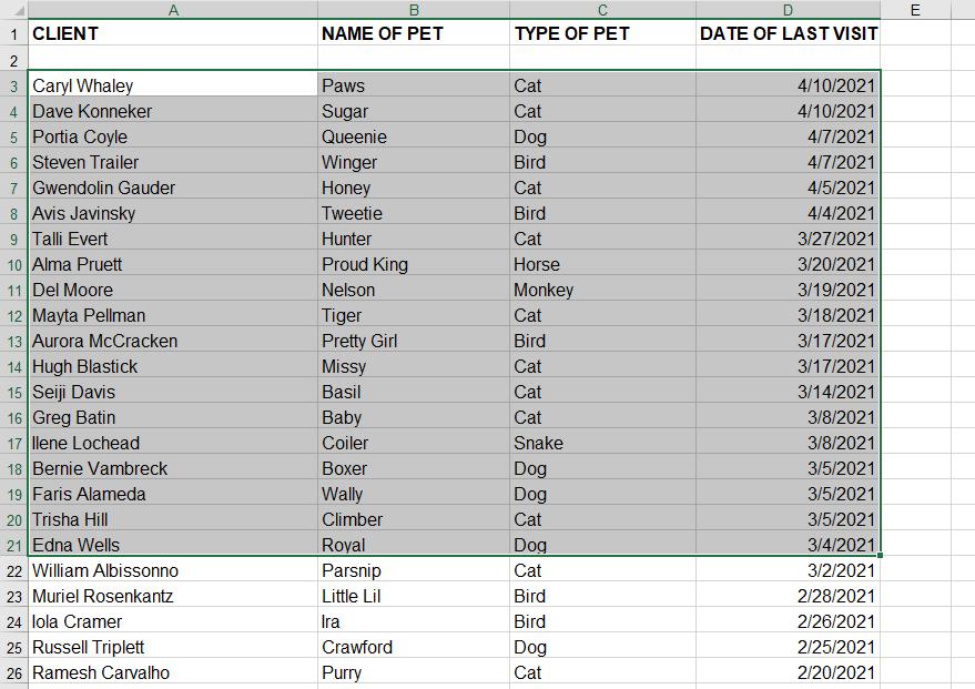
A range is usually a group of adjacent cells, although noncontiguous cells can be included in the same range (but that’s mostly for rocket scientists and those obsessed with treating data like jigsaw puzzle pieces). For your purposes, assume a range is a group of continuous cells. Make a range right now! Here’s how:
1. Position the mouse pointer over the first cell where you want to define a range.
2. Press and hold the left mouse button.
3. Move the pointer to the last cell of your desired area.
4. Release the mouse button.
Figure 1-8 shows what happened when I did this. I selected a range of cells. The address of this range is A3:D21.
FIGURE 1-9: Adding a name to the workbook.
A range address looks like two cell addresses put together, with a colon (:) in the middle. And that’s what it is! A range address starts with the address of the cell in the upper left of the range, then has a colon, and ends with the address of the cell in the lower right.
One more detail about ranges: You can give them a name. This is a great feature because you can think about a range in terms of what it is used for, instead of what its address is. Also, if I did not take the extra step to assign a name, the range would be gone as soon as I clicked anywhere on the worksheet. When a range is given a name, you can repeatedly use the range by using its name.
Say you have a list of clients on a worksheet. What’s easier — thinking of exactly which cells are occupied, or thinking that there is your list of clients?
Throughout this book, I use areas made of cell addresses and ranges, which have been given names. It’s time to get your feet wet creating a named area. Here’s what you do:
1. Position the mouse pointer over a cell, click and hold the left mouse button, and drag the pointer around.
2. Release the mouse button when you’re done.
You’ve selected an area of the worksheet.
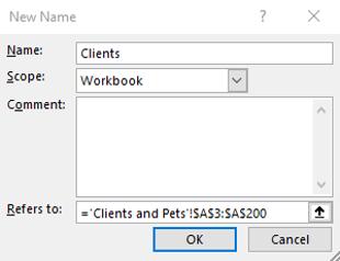
3. Click Define Name in the Defined Names group on the Formulas tab.
The New Name dialog box appears. Figure 1-9 shows you how it looks so far.
4. Name the area or keep the suggested name. You can change the suggested name as well.
Excel guesses that you want to name the area with the value it finds in the top cell of the range. That may or may not be what you want. Change the name if you need to. In Figure 1-9, I changed the name to Clients.