Data Ingestion with Python Cookbook: A practical guide to ingesting, monitoring, and identifying errors in the data ingestion process 1st Edition Esppenchutz
Exploratory Data Analysis with Python Cookbook: Over 50 recipes to analyze, visualize, and extract insights from structured and unstructured data Oluleye
All rights reserved. No part of this book may be reproduced, stored in a retrieval system, or transmitted in any form or by any means, without the prior written permission of the publisher, except in the case of brief quotations embedded in critical articles or reviews.
Every effort has been made in the preparation of this book to ensure the accuracy of the information presented. However, the information contained in this book is sold without warranty, either express or implied. Neither the author, nor Packt Publishing, and its dealers and distributors will be held liable for any damages caused or alleged to be caused directly or indirectly by this book.
Packt Publishing has endeavored to provide trademark information about all of the companies and products mentioned in this book by the appropriate use of capitals. However, Packt Publishing cannot guarantee the accuracy of this information.
Early Access Publication: Python Data Cleaning Cookbook
Early Access Production Reference: B18596
Published by Packt Publishing Ltd.
Livery Place 35 Livery Street Birmingham B3 2PB, UK
ISBN: 978-1-80323-987-3
Table of Contents
1. Python Data Cleaning Cookbook, Second Edition: Detect and remove dirty data and extract key insights with pandas, machine learning and ChatGPT, Spark, and more
2. 1 Anticipating Data Cleaning Issues when Importing Tabular Data into Pandas
I. Join our book community on Discord
II. Importing CSV files
i. Getting ready
ii. How to do it…
iii. How it works...
iv. There’s more...
v. See also
III. Importing Excel files
i. Getting ready
ii. How to do it…
iii. How it works…
iv. There’s more…
v. See also
IV. Importing data from SQL databases
i. Getting ready
ii. How to do it...
iii. How it works…
iv. There’s more…
v. See also
V. Importing SPSS, Stata, and SAS data
i. Getting ready
ii. How to do it...
iii. How it works...
iv. There’s more…
v. See also
VI. Importing R data
i. Getting ready
ii. How to do it…
iii. How it works…
iv. There’s more…
v. See also
VII. Persisting tabular data
i. Getting ready
ii. How to do it…
iii. How it works...
iv. There’s more...
3. 2 Anticipating Data Cleaning Issues when Working with HTML, JSON, and Spark Data
I. Join our book community on Discord
II. Importing simple JSON data
i. Getting ready…
ii. How to do it…
iii. How it works…
iv. There’s more…
III. Importing more complicated JSON data from an API
i. Getting ready…
ii. How to do it...
iii. How it works…
iv. There’s more…
v. See also
IV. Importing data from web pages
i. Getting ready...
ii. How to do it…
iii. How it works…
iv. There’s more…
V. Working with Spark data
i. Getting ready...
ii. How it works...
iii. There’s more...
VI. Persisting JSON data
i. Getting ready…
ii. How to do it...
iii. How it works…
iv. There’s more…
4. 3 Taking the Measure of Your Data
I. Join our book community on Discord
II. Getting a first look at your data
i. Getting ready…
ii. How to do it...
iii. How it works…
iv. There’s more...
v. See also
III. Selecting and organizing columns
i. Getting Ready…
ii. How to do it…
iii. How it works…
iv. There’s more…
v. See also
IV. Selecting rows
i. Getting ready...
ii. How to do it...
iii. How it works…
iv. There’s more…
v. See also
V. Generating frequencies for categorical variables
i. Getting ready…
ii. How to do it…
iii. How it works…
iv. There’s more…
VI. Generating summary statistics for continuous variables
i. Getting ready…
ii. How to do it…
iii. How it works…
iv. See also
VII. Using generative AI to view our data
i. Getting ready…
ii. How to do it…
iii. How it works…
iv. See also
5. 4 Identifying Missing Values and Outliers in Subsets of Data
I. Join our book community on Discord
II. Finding missing values
i. Getting ready
ii. How to do it…
iii. How it works...
iv. See also
III. Identifying outliers with one variable
i. Getting ready
ii. How to do it...
iii. How it works…
iv. There’s more…
v. See also
IV. Identifying outliers and unexpected values in bivariate relationships
i. Getting ready
ii. How to do it...
iii. How it works…
iv. There’s more…
v. See also
V. Using subsetting to examine logical inconsistencies in variable relationships
i. Getting ready
ii. How to do it…
iii. How it works…
iv. See also
VI. Using linear regression to identify data points with significant influence
i. Getting ready
ii. How to do it…
iii. How it works...
iv. There’s more…
VII. Using K-nearest neighbor to find outliers
i. Getting ready
ii. How to do it…
iii. How it works...
iv. There’s more...
v. See also
VIII. Using Isolation Forest to find anomalies
i. Getting ready
ii. How to do it...
iii. How it works…
iv. There’s more…
v. See also
6. 5 Using Visualizations for the Identification of Unexpected Values
I. Join our book community on Discord
II. Using histograms to examine the distribution of continuous variables
i. Getting ready
ii. How to do it…
iii. How it works…
iv. There’s more...
III. Using boxplots to identify outliers for continuous variables
i. Getting ready
ii. How to do it…
iii. How it works...
iv. There’s more...
v. See also
IV. Using grouped boxplots to uncover unexpected values in a particular group
i. Getting ready
ii. How to do it...
iii. How it works...
iv. There’s more…
v. See also
V. Examining both distribution shape and outliers with violin plots
i. Getting ready
ii. How to do it…
iii. How it works…
iv. There’s more…
v. See also
VI. Using scatter plots to view bivariate relationships
i. Getting ready
ii. How to do it...
iii. How it works…
iv. There’s more...
v. See also
VII. Using line plots to examine trends in continuous variables
i. Getting ready
ii. How to do it…
iii. How it works...
iv. There’s more…
v. See also
VIII. Generating a heat map based on a correlation matrix
i. Getting ready
ii. How to do it…
iii. How it works…
iv. There’s more…
v. See also
Python Data Cleaning Cookbook, Second Edition: Detect and remove dirty data and extract key insights with pandas, machine learning and ChatGPT, Spark, and more
Welcome to Packt Early Access. We’re giving you an exclusive preview of this book before it goes on sale. It can take many months to write a book, but our authors have cutting-edge information to share with you today. Early Access gives you an insight into the latest developments by making chapter drafts available. The chapters may be a little rough around the edges right now, but our authors will update them over time.You can dip in and out of this book or follow along from start to finish; Early Access is designed to be flexible. We hope you enjoy getting to know more about the process of writing a Packt book.
1. Chapter 1: Anticipating Data Cleaning Issues when Importing Tabular Data into Pandas
2. Chapter 2: Anticipating Data Cleaning Issues when Working with HTML, JSON, and Spark Data
3. Chapter 3: Taking the Measure of Your Data
4. Chapter 4: Identifying Missing Values and Outliers in Subsets of Data
5. Chapter 5: Using Visualizations for the Identification of Unexpected Values
6. Chapter 6: Cleaning and Exploring Data with Series Operations
7. Chapter 7: Working with Missing Data
8. Chapter 8: Fixing Messy Data When Aggregating
9. Chapter 9: Addressing Data Issues When Combining Data Frames
10. Chapter 10: Tidying and Reshaping Data
11. Chapter 11: Automate Data Cleaning with User-Defined Functions and
1 Anticipating Data Cleaning Issues
when Importing Tabular Data into Pandas
Join our book community on Discord
https://discord.gg/28TbhyuH
Scientific distributions of Python (Anaconda, WinPython, Canopy, and so on) provide analysts with an impressive range of data manipulation, exploration, and visualization tools. One important tool is pandas. Developed by Wes McKinney in 2008, but really gaining in popularity after 2012, pandas is now an essential library for data analysis in Python. We work with pandas extensively in this book, along with popular packages such as numpy , matplotlib , and scipy .A key pandas object is the DataFrame, which represents data as a tabular structure, with rows and columns. In this way, it is similar to the other data stores we discuss in this chapter. However, a pandas DataFrame also has indexing functionality that makes selecting, combining, and transforming data relatively straightforward, as the recipes in this book will demonstrate.Before we can make use of this great functionality, we have to get our data into pandas. Data comes to us in a wide variety of formats: as CSV or Excel files, as tables from SQL databases, from statistical analysis packages such as SPSS, Stata, SAS, or R, from non-tabular sources such as JSON, and from web pages.We examine tools for importing tabular data in this recipe. Specifically, we cover the following topics:
Importing CSV files
Importing Excel files
Importing data from SQL databases
Importing SPSS, Stata, and SAS data
Importing R data
Persisting tabular data
Importing CSV files
The read csv method of the pandas library can be used to read a file with comma separated values (CSV) and load it into memory as a pandas DataFrame. In this recipe, we read a CSV file and address some common issues: creating column names that make sense to us, parsing dates, and dropping rows with critical missing data.Raw data is often stored as CSV files. These files have a carriage return at the end of each line of data to demarcate a row, and a comma between each data value to delineate columns. Something other than a comma can be used as the delimiter, such as a tab. Quotation marks may be placed around values, which can be helpful when the delimiter occurs naturally within certain values, which sometimes happens with commas.All data in a CSV file are characters, regardless of the logical data type. This is why it is easy to view a CSV file, presuming it is not too large, in a text editor. The pandas read csv method will make an educated guess about the data type of each column, but you will need to help it along to ensure that these guesses are on the mark.
Getting ready
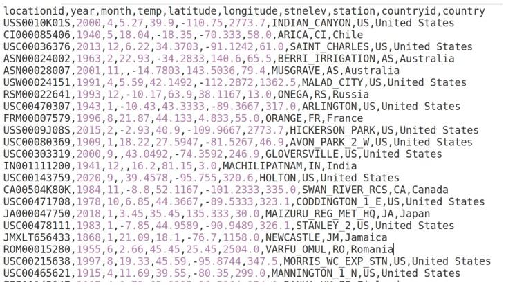
Create a folder for this chapter and create a new Python script or Jupyter Notebook file in that folder. Create a data subfolder and place the landtempssample.csv file in that subfolder. Alternatively, you could retrieve all of the files from the GitHub repository. Here is a screenshot of the beginning of the CSV file:
Note
This dataset, taken from the Global Historical Climatology Network integrated database, is made available for public use by the United States National Oceanic and Atmospheric Administration at https://www.ncdc.noaa.gov/data-access/landbased-station-data/land-based-datasets/global-historicalclimatology-network-monthly-version-4. This is just a 100,000-row sample of the full dataset, which is also available in the repository.
How to do it…
We will import a CSV file into pandas, taking advantage of some very useful read csv options:
1. Import the pandas library and set up the environment to make viewing the output easier:
import pandas as pd pd.options.display.float format = '{:,.2f}'.format
Figure 1.1: Land Temperatures Data
pd.set option('display.width', 85)
pd.set option('display.max columns', 8)
1. Read the data file, set new names for the headings, and parse the date column.
Pass an argument of 1 to the skiprows parameter to skip the first row, pass a list of columns to parse dates to create a pandas datetime column from those columns, and set low memory to False to reduce the usage of memory during the import process:
We have to use skiprows because we are passing a list of column names to read csv . If we use the column names in the CSV file we do not need to specify values for either names or skiprows .
1. Get a quick glimpse of the data.
View the first few rows. Show the data type for all columns, as well as the number of rows and columns:
>>> landtemps.head(7) month year stationid ... countryid \
0 2000-04-01 USS0010K01S ... US
1 1940-05-01 CI000085406 ... CI
2 2013-12-01 USC00036376 ... US
3 1963-02-01 ASN00024002 ...
4 2001-11-01 ASN00028007 ... AS
5 1991-04-01 USW00024151 ... US
6 1993-12-01 RSM00022641 ... RS country
[7 rows x 9 columns]
>>> landtemps.dtypes
month year datetime64[ns]
stationid object
avgtemp float64
latitude float64
longitude float64
elevation float64
station object
countryid object country object
dtype: object
>>> landtemps.shape
(100000, 9)
1. Give the date column a better name and view the summary statistics for average monthly temperature:
Use isnull , which returns True for each value that is missing for each column, and False when not missing. Chain this with sum to count the missings for each column. (When working with Boolean values, sum treats True as 1 and False as 0 . I will discuss method chaining in the There’s more... section of this recipe):
>>> landtemps.isnull().sum()
measuredate 0
stationid 0
avgtemp 14446
latitude 0
longitude 0
elevation 0
station 0
countryid 0
country 5 dtype: int64
1. Remove rows with missing data for avgtemp .
Use the subset parameter to tell dropna to drop rows when avgtemp is missing. Set inplace to True . Leaving inplace at its default value of False would display the DataFrame, but the changes we have made would not be retained. Use the shape attribute of the DataFrame to get the number of rows and columns:
That’s it! Importing CSV files into pandas is as simple as that.
How it works...
Almost all of the recipes in this book use the pandas library. We refer to it as pd to make it easier to reference later. This is customary. We also use float format to display float values in a readable way and set option to make the terminal output wide enough to accommodate the number of variables.Much of the work is done by the first line in step 2. We use read csv to load a pandas DataFrame in memory and call it landtemps . In addition to passing a filename, we set the names parameter to a list of our preferred column headings. We also tell read csv to skip the first row, by setting skiprows to 1, since the original column headings are in the first row of the CSV file. If we do not tell it to skip the first row, read csv will treat the header row in the file as actual data. read csv also solves a date conversion issue for us. We use the parse dates parameter to ask it to convert the month and year columns to a date value.Step 3 runs through a few standard data checks. We use head(7) to print out all columns for the first 7 rows. We use the dtypes attribute of the data frame to show the data type of all columns. Each column has the expected data type. In pandas, character data has the object data type, a data type that allows for mixed values. shape returns a tuple, whose first element is the number of rows in the data frame (100,000 in this case) and whose second element is the number of columns (9).When we used read csv to parse the month and year columns, it gave the resulting column the name month year . We use the rename method in step 4 to give that column a better name. We need to specify inplace=True to replace the old column name with the new column name in memory. The describe method provides summary statistics on the avgtemp column.Notice that the count for avgtemp indicates that there are 85,554 rows that have valid values for avgtemp . This is out of 100,000 rows for the whole DataFrame, as provided by the shape attribute. The listing of missing values for each column in step 5 ( landtemps.isnull().sum() ) confirms this: 100,000 – 85,554 = 14,446.Step 6 drops all rows where avgtemp is NaN . (The NaN value, not a number, is the pandas representation of missing values.) subset is used to indicate which column to check for missings. The shape attribute for landtemps now indicates that there are 85,554 rows, which is what we would expect given the previous count from describe .
There’s more...
If the file you are reading uses a delimiter other than a comma, such as a tab, this can be specified in the sep parameter of read csv . When creating the pandas DataFrame, an index was also created. The numbers to the far left of the output when head and sample were run are index values. Any number of rows can be specified for head or sample . The default value is 5 .Setting low memory to False causes read csv to parse data in chunks. This is easier on systems with lower memory when working with larger files. However, the full DataFrame will still be loaded into memory once read csv completes successfully.The landtemps.isnull().sum() statement is an example of chaining methods. First, isnull returns a DataFrame of True and False values, resulting from testing whether each column value is null . sum takes that DataFrame and sums the True values for each column, interpreting the True values as 1 and the False values as 0 . We would have obtained the same result if we had used the following two steps:
>>> checknull = landtemps.isnull()
>>> checknull.sum()
There is no hard and fast rule for when to chain methods and when not to do so. I find it helpful to chain when I really think of something I am doing as being a single step, but only two or more steps, mechanically speaking. Chaining also has the side benefit of not creating extra objects that I might not need.The dataset used in this recipe is just a sample from the full land temperatures database with almost 17 million records. You can run the larger file if your machine can handle it, with the following code:
>>> landtemps = pd.read csv('data/landtemps.zip',
... compression='zip', names=['stationid','year',
... 'month','avgtemp','latitude','longitude',
... 'elevation','station','countryid','country'],
... skiprows=1,
... parse dates=[['month','year']],
... low memory=False)
read csv can read a compressed ZIP file. We get it to do this by passing the name of the ZIP file and the type of compression.
See also
Subsequent recipes in this chapter, and in other chapters, set indexes to improve navigation over rows and merging.A significant amount of reshaping of the Global Historical Climatology Network raw data was done before using it in this recipe. We demonstrate this in Chapter 8, Tidying and Reshaping Data.
Importing Excel files
The read excel method of the pandas library can be used to import data from an Excel file and load it into memory as a pandas DataFrame. In this recipe, we import an Excel file and handle some common issues when working with Excel files: extraneous header and footer information, selecting specific columns, removing rows with no data, and connecting to particular sheets.Despite the tabular structure of Excel, which invites the organization of data into rows and columns, spreadsheets are not datasets and do not require people to store data in that way. Even when some data conforms with those expectations, there is often additional information in rows or columns before or after the data to be imported. Data types are not always as clear as they are to the person who created the spreadsheet. This will be all too familiar to anyone who has ever battled with importing leading zeros. Moreover, Excel does not insist that all data in a column be of the same type, or that column headings be appropriate for use with a programming language such as Python.Fortunately, read excel has a number of options for handling messiness in Excel data. These options make it relatively easy to skip rows and select particular columns, and to pull data from a particular sheet or sheets.
Getting ready
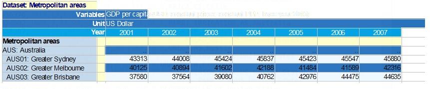
You can download the GDPpercapita.xlsx file, as well as the code for this recipe, from the GitHub repository for this book. The code assumes that the Excel file is in a data subfolder. Here is a view of the beginning of the file:
Figure 1.2: View of the dataset
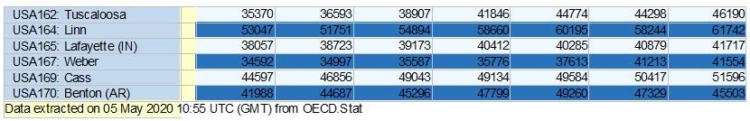
And here is a view of the end of the file:
1.3: View of the dataset
Note
This dataset, from the Organisation for Economic Co-operation and Development, is available for public use at https://stats.oecd.org/.
How to do it…
We import an Excel file into pandas and do some initial data cleaning:
1. Import the pandas library:
>>> import pandas as pd
1. Read the Excel per capita GDP data.
Select the sheet with the data we need, but skip the columns and rows that we do not want. Use the sheet name parameter to specify the sheet. Set skiprows to 4 and skipfooter to 1 to skip the first four rows (the first row is hidden) and the last row. We provide values for usecols to get data from column A and columns C through T (column B is blank). Use head
1. Use the info method of the data frame to view data types and the non-null count:
>>> percapitaGDP.info()
<class 'pandas.core.frame.DataFrame'>
RangeIndex: 702 entries, 0 to 701
Data columns (total 19 columns): # Column Non-Null Count Dtype
object
object
object
object
object
memory usage: 104.3+ KB
1. Rename the Year column to metro and remove the leading spaces.
Give an appropriate name to the metropolitan area column. There are extra spaces before the metro values in some cases, and extra spaces after the metro values in others. We can test for leading spaces with startswith(‘ ‘) and then use any to establish whether there are one or more occasions when the first character is blank. We can use endswith(‘ ‘) to examine trailing spaces. We use strip to remove both leading and trailing spaces. When we test for trailing spaces again we see that there are none:
Iterate over all of the GDP year columns (2001-2018) and convert the data type from object to float . Coerce the conversion even when there is character data – the .. in this example. We want character values in those columns to become missing, which is what happens. Rename the year columns to better reflect the data in those columns:
std 11878 12537 15464 15720 min 10988 11435 2745 2832
25% 33139 32636 37316 37908
50% 39544 39684 45385 46057
75% 47972 48611 56023 56638
max 91488 93566 122242 127468
[8 rows x 18 columns]
1. Remove rows where all of the per capita GDP values are missing.
Use the subset parameter of dropna to inspect all columns, starting with the second column (it is zero-based) through the last column. Use how to specify that we want to drop rows only if all of the columns specified in subset are missing. Use shape to show the number of rows and columns in the resulting DataFrame:
We have now imported the Excel data into a pandas data frame and cleaned up some of the messiness in the spreadsheet.
How it works…
We mostly manage to get the data we want in step 2 by skipping rows and columns we do not want, but there are still a number of issues: read excel interprets all of the GDP data as character data, many rows are loaded with no useful data, and the column names do not represent the data well. In addition, the metropolitan area column might be useful as an index, but there are leading and trailing blanks and there may be missing or duplicated values. read excel interprets Year as the column name for the metropolitan area data because it looks for a header above the data for that Excel column and finds Year there. We rename that column metro in step 4. We also use strip to fix the problem with leading and trailing blanks. If there had only been leading blanks, we could have used lstrip , or rstrip if there had only been trailing blanks. It is a good idea to assume that there might be leading or trailing blanks in any character data and clean that data shortly after the initial import.The spreadsheet authors used .. to represent missing data. Since this is actually valid character data, those columns get the object data type (that is how pandas treats columns with character or mixed data). We coerce a conversion to numeric in step 5. This also results in the original values of .. being replaced with NaN (not a number), pandas missing values for numbers. This is what we want.We can fix all of the per capita GDP columns with just a few lines because pandas makes it easy to iterate over the