https://ebookmass.com/product/statistics-for-ecologists-
Instant digital products (PDF, ePub, MOBI) ready for you
Download now and discover formats that fit your needs...
eTextbook 978-0134173054 Statistics for Managers Using Microsoft Excel
https://ebookmass.com/product/etextbook-978-0134173054-statistics-formanagers-using-microsoft-excel/
ebookmass.com
Advances in Business Statistics, Methods and Data Collection Ger Snijkers
https://ebookmass.com/product/advances-in-business-statistics-methodsand-data-collection-ger-snijkers/
ebookmass.com
Using Statistics in the Social and Health Sciences with SPSS Excel 1st…
https://ebookmass.com/product/using-statistics-in-the-social-andhealth-sciences-with-spss-excel-1st/
ebookmass.com
Oral Pathology for the Dental Hygienist E Book 7th Edition, (Ebook PDF)
https://ebookmass.com/product/oral-pathology-for-the-dental-hygieniste-book-7th-edition-ebook-pdf/
ebookmass.com
Polar Organometallic Reagents - Synthesis, Structure, Properties and Applications Wheatley Andrew E.H. (Ed.)
https://ebookmass.com/product/polar-organometallic-reagents-synthesisstructure-properties-and-applications-wheatley-andrew-e-h-ed/
ebookmass.com
The Stormbringer Isabel Cooper [Cooper
https://ebookmass.com/product/the-stormbringer-isabel-cooper-cooper/
ebookmass.com
The Bourgeois and the Savage: A Marxian Critique of the Image of the Isolated Individual in Defoe, Turgot and Smith Iacono Alfonso Maurizio
https://ebookmass.com/product/the-bourgeois-and-the-savage-a-marxiancritique-of-the-image-of-the-isolated-individual-in-defoe-turgot-andsmith-iacono-alfonso-maurizio/
ebookmass.com
Surfeit of Suspects George Bellairs
https://ebookmass.com/product/surfeit-of-suspects-george-bellairs/
ebookmass.com
Interviewing and Change Strategies for Helpers 8th Edition
Sherry Cormier
https://ebookmass.com/product/interviewing-and-change-strategies-forhelpers-8th-edition-sherry-cormier/
ebookmass.com
Communicating Across Cultures and Languages in the Health Care Setting: Voices of Care 1st Edition Claire Penn
https://ebookmass.com/product/communicating-across-cultures-andlanguages-in-the-health-care-setting-voices-of-care-1st-editionclaire-penn/
ebookmass.com
Preface
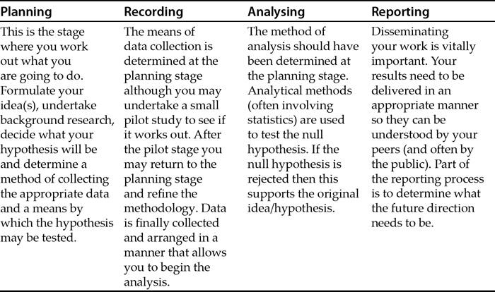
1. Planning
1.1 The scientific method
1.2 Types of experiment/project
1.3 Getting data – using a spreadsheet
1.4 Hypothesis testing
1.5 Data types
1.6 Sampling effort
1.7 Tools of the trade
1.8 The R program
1.9 Excel
2. Data recording
2.1 Collecting data – who, what, where, when
2.2 How to arrange data
3. Beginning data exploration – using software tools
3.1 Beginning to use R
3.2 Manipulating data in a spreadsheet
3.3 Getting data fromExcel into R
4. Exploring data – looking at numbers
4.1 Summarizing data
4.2 Distribution
4.3 Anumerical value for the distribution
4.4 Statistical tests for normal distribution
4.5 Distribution type
4.6 Transforming data
4.7 When to stop collecting data? The running average
4.8 Statistical symbols
5. Exploring data – which test is right?
5.1 Types of project
5.2 Hypothesis testing
5.3 Choosing the correct test
6. Exploring data – using graphs
6.1 Introduction to data visualization
6.2 Exploratory graphs
6.3 Graphs to illustrate differences
6.4 Graphs to illustrate correlation and regression
6.5 Graphs to illustrate association
6.6 Graphs to illustrate similarity
6.7 Graphs – a summary
7. Tests for differences
7.1 Differences: t-test
7.2 Differences: U-test
7.3 Paired tests
8. Tests for linking data – correlations
8.1 Correlation: Spearman’s rank test
8.2 Pearson’s product moment
8.3 Correlation tests using Excel
8.4 Correlation tests using R
8.5 Curved linear correlation
9. Tests for linking data – associations
9.1 Association: chi-squared test
9.2 Goodness of fit test
9.3 Using R for chi-squared tests
9.4 Using Excel for chi-squared tests
10. Differences between more than two samples
10.1 Analysis of variance
10.2 Kruskal–Wallis test
11. Tests for linking several factors
11.1 Multiple regression
11.2 Curved-linear regression
11.3 Logistic regression
12. Community ecology
12.1 Diversity
12.2 Similarity
13. Reporting results
13.1 Presenting findings
13.2 Publishing
13.3 Reporting results of statistical analyses
13.4 Graphs
13.5 Writing papers
13.6 Plagiarism
13.7 References
13.8 Poster presentations
13.9 Giving a talk (PowerPoint)
14. Summary
Glossary Appendices
Index
1.2 Types of experiment/project
As part of the planning process, you need to be aware of what you are trying to achieve. In general, there are three main types of research:
• Differences: you look to show that a is different to b and perhaps that c is different again. These kinds of situations are represented graphically using bar charts and box–whisker plots.
• Correlations: you are looking to find links between things. This might be that species a has increased in range over time or that the abundance of species a (or environmental factor a) affects the abundance of species b. These kinds of situations are represented graphically using scatter plots.
• Associations: similar to the above except that the type of data is a bit different, e.g. species a is always found growing in the same place as species b. These kinds of situations are represented graphically using pie charts and bar charts.
Studies that concern whole communities of organisms usually require quite different approaches. The kinds of approach required for the study of community ecology are dealt with
in detail in the companion volume to this work (Community Ecology, Analytical Methods Using R and Excel, Gardener 2014).
In this volume you’ll see some basic approaches to community ecology, principally diversity and sample similarity (see Chapter 12). The other statistical approaches dealt with in this volume underpin many community studies.
Once you know what you are aiming at, you can decide what sort of data to collect; this affects the analytical approach, as you shall see later. You’ll return to the topic of project types in Chapter 5.
1.3 Getting data – using a spreadsheet
A spreadsheet is an invaluable tool in science and data analysis. Learning to use one is a good skill to acquire. With a spreadsheet you are able to manipulate data and summarize it in different ways quite easily. You can also prepare data for further analysis in other computer programs in a spreadsheet. It is important that you formalize the data into a standard format, as you’ll see later (in Chapter 2). This will make the analysis run smoothly and allow others to follow what you have done. It will also allow you to see what you did later on (it is easy to forget the details).
Your spreadsheet is useful as part of the planning process. You may need to look at old data; these might not be arranged in an appropriate fashion, so using the spreadsheet will allow you to organize your data. The spreadsheet will allow you to perform some simple manipulations and run some straightforward analyses, looking at means, for example, as well as producing simple summary graphs. This will help you to understand what data you have and what they might show. You’ll look at a variety of ways of manipulating data later (see Section 3.2).
If you do not have past data and are starting from scratch, then your initial site visits and pilot studies will need to be dealt with. The spreadsheet should be the first thing you look to, as this will help you arrange your data into a format that facilitates further study. Once you have some initial data (be it old records or pilot data) you can continue with the planning process.
1.4 Hypothesis testing
A hypothesis is your idea of what you are trying to determine. Ideally it should relate to a single thing, so “Japanese knotweed and Himalayan balsam have increased their range in the UK over the past 10 years” makes a good overall aim, but is actually two hypotheses. You should split up your ideas into parts, each of which can be tested separately:
“Japanese knotweed has increased its range in the UK over the past 10 years.”
“Himalayan balsamhas increased its range in the UK over the past 10 years.”
You can think of hypothesis testing as being like a court of law. In law, you are presumed innocent until proven guilty; you don’t have to prove your innocence.
In statistics, the equivalent is the null hypothesis. This is often written as H0 (or H0) and you aim to reject your null hypothesis and therefore, by implication, accept the alternative (usually written as H1 or H1).
The H0 is not simply the opposite of what you thought (called the alternative hypothesis, H1) but is written as such to imply that no difference exists, no pattern (I like to think of it as the dull hypothesis). For your ideas above you would get:
“There has been no change in the range of Japanese knotweed in the UK over the past 10 years.”
“There has been no change in the range of Himalayan balsam in the UK over the past 10 years.”
So, you do not say that the range of these species is shrinking, but that there is no change. Getting your hypotheses correct (and also the null hypotheses) is an important step in the planning process as it allows you to decide what data you will need to collect in order to reject the H0. You’ll examine hypotheses in more detail later (Section 5.2).
1.4.1 Hypothesis and analytical methods
Allied to your hypothesis is the analytical method you will use to help test and support (or otherwise) your hypothesis. Even at this early stage you should have some idea of the statistical test you are going to apply. Certain statistical tests are suitable for certain kinds of data and you can therefore make some early decisions. You may alter your approach, change the method of analysis and even modify your hypothesis as you move through the planning stages: this all part of the scientific process. You’ll look at ways to choose which statistical test is right for your situation in Section 5.3, where you will see a decision flow-chart (Figure 5.1) and a key (Table 5.1) to help you. Before you get to that stage, though, you will need to think a little more about the kind of data you may collect.
1.5 Data types
Once you have sorted out more or less what your hypotheses are, the next step in the planning process is to determine what sort of data you can get. You may already have data from previous biological records or some other source. Knowing what sort of data you have will determine the sorts of analyses you are able to perform. In general, you can have three main types of data:
• Interval: these can be thought of as “real” numbers. You know the sizes of them and can do “proper” mathematics. Examples would be counts of invertebrates, percentage cover, leaf lengths, egg weights, or clutch size.
• Ordinal: these are values that can be placed in order of size but that is pretty much all you can do. Examples would be abundance scales like DAFOR or Domin (named after a Czech
botanist). You know that A is bigger than O but you cannot say that one is twice as big as the other (or be exact about the difference).
• Categorical (sometimes called nominal data): this is the tricky one because it can be confused with ordinal data. With categorical data you can only say that things are different. Examples would be flower colour, habitat type, or sex.
With interval data, for example, you might count something, keep counting and build up a sample. When you are finished, you can take your list and calculate an average, look to see how much larger the biggest value is from the smallest and so on. Put another way, you have a scale of measurement. This scale might be millimetres or grams or anything else. Whenever you measure something using this scale you can see how it fits into the scheme of things because the interval of your scale is fixed (10 mm is bigger than 5 mm, 4 g is less than 12 g). Compare this to the ordinal scales described below.
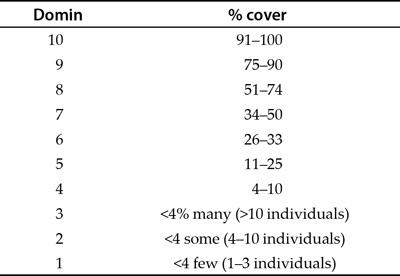
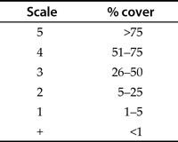
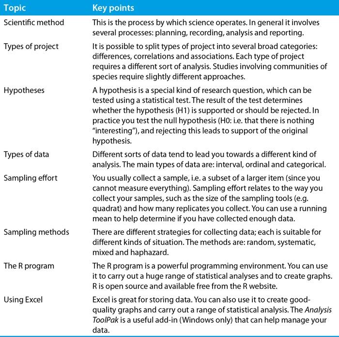
With ordinal data you might look at the abundance of a species in quadrats. It may be difficult or time consuming to be exact so you decide to use an abundance scale. The Domin scale shown in Table 1.2, for example, converts percentage cover into a numerical value from 0 to 10.
Table 1.2 The Domin scale; an example of an ordinal abundance scale.
The Domin scale is generally used for looking at plant abundance and is used in many kinds of study. You can see by looking at Table 1.2 that the different classifications cover different ranges of abundance. For example, a Domin of 8 represents a range of values from about half to three-quarters coverage (51–74%). A value of 6 represents a range fromabout a quarter to a third coverage (26–33%). The first three divisions of the Domin scale all represent less than 4% coverage but relate to the number of individuals found. The Domin scale is useful because it allows you to collect data efficiently and still permits useful analysis. You know that 10 is a
greater percentage coverage than 8 and that 8 is bigger than 6; it is just that the intervals between the divisions are unequal.
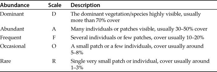
Table 1.3 An example of a generalized DAFOR scale for vegetation, an example of an ordinal abundance scale.
There are many other abundance scales, and various researchers have at times worked out useful ways to simplify the abundance of organisms. The DAFOR scale is a general phrase to describe abundance scales that convert abundance into a letter code. There are many examples. Table 1.3 shows a generalized scale for vegetation analysis.
There are other letters that might be used to extend your scale. For example C for “common” might be inserted between Aand F (ACFOR is a commonly used ordinal scale). You might add E and/or S for “extremely abundant” and “super abundant”. You might also add N for “not found”. The DAFOR type of scale can be used for any organism, not just for vegetation.
When you are finished, you can convert your DAFOR scale into numbers (ranks) and get an average, which can be converted to a DAFOR letter, but you cannot tell how much larger the biggest is fromthe smallest – the interval between the values is inexact.
Many of the abundance scales used are derived from the work of Josias Braun-Blanquet, an eminent Swiss botanist. Table 1.4 shows a basic example of a Braun-Blanquet scale for vegetation cover.
Table 1.4 The basic Braun-Blanquet scale, an ordinal abundance scale. There are many variations on this scale.
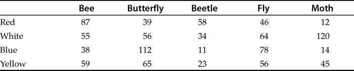
With categorical data it is useful to think of an example. You might go out and look to see what types of insect are visiting different colours of flower. Every time you spot an insect, you record its type (bee, fly, beetle) and the flower colour. At the end you can make a table with numbers of how many of each type visited each colour. You have numbers but each value is uniquely a combination of two categories.
Table 1.5 shows an example of categorical data laid out in what is called a contingency table. The rows are one category (colour) and the columns another category (type of insect).
Table 1.5 An example of categorical data. This type of table is also called a contingency table. The rows and columns are each sets of categories. Each cell of the table represents a unique combination of categories.
1.6 Sampling effort
Sampling effort refers to the way you collect data and how much to collect. For example, you have decided that you need to determine the abundance of some plant species in meadows across lowland Britain. How many quadrats will you use? How large will the quadrats need to be? Do you need quadrats at all?
Sample is the term used to describe the set of data that you have. Because you generally cannot measure “everything”, you will usually have a subset of stuff that you’ve measured (or weighed or counted). Think about a field of buttercups as an example. You wish to know how many there are in the field, which is a hectare in size (i.e. 100 m × 100 m). You aren’t really
going to count them all (that would take too long) so you make up a square that has sides of 1 metre and count how many buttercups there are in that. Now you can estimate how many buttercups there are in the whole field. Your sample is 1/10,000th of the area, which is pretty small. The estimate is not likely to be very good (although by random chance it could be). It seems reasonable to count buttercups in a few more 1 m2 areas. In this way your estimate is likely to get more “on target”. Think of it this way: if you carried on and on and on, eventually you would have counted buttercups in every 1 m2 of the field. Your estimate would now be spot on because you would have counted everything. So as you collect more and more data, your estimate of the true number of buttercups will likely become more and more like the true number.
The problem is, how many 1 m2 areas will you have to count in order to get a good estimate of the true number? You will return to this issue a little later. Another problem – where do you put your 1 m2 areas? Will it make a difference? Is a 1 m2 quadrat the right size? You will look at these themes now.
1.6.1 Quadrat size
If you are doing a British NVC survey, then the size and number of quadrats is predetermined; the NVC methodology is standardized. Similarly, if you are making bird species lists for different sites, the methodology already exists for you to follow. Don’t reinvent the wheel! Whenever you collect data, you cannot measure everything, so you take a sample, essentially a representative subset of the whole. What you are aiming for is to make your sample as representative as possible. If, for example, you were counting the frequency of spider orchids across a site, you would aim to make your quadrat a reasonable size and in line with the size and distribution of the organism – you would not have the same size quadrat to look at oak trees as you would to look at lichens.
1.6.2 Species area rule
If you are looking at communities, then the wider the area you cover the more species you will find. Imagine you start off with a tiny quadrat: you might just find a few species. Make the quadrat double the size and you will find more. Keep doubling the quadrat and you will keep finding more species. If, however, you draw a graph of the cumulative number of species, you will see it start to level off and eventually you won’t find any more species. Even well before this, the number of new species will be so small that it is not worth the extra effort of the larger quadrat. This idea is called the species area rule. You’ll see more details about community studies in Chapter 12.
You can extend the same idea to kick-sampling, which is a method for collecting freshwater invertebrates. You use a standard net for freshwater invertebrate sampling but can vary the time you spend sampling. This is akin to using a bigger quadrat. The longer you sample, the more you get. You can easily see that it is not worth spending 20 minutes to get the 101st species when during 3 minutes you net the first 100.
1.6.3 How many replicates?
When you go out to collect your data, how much work do you have to do? If you are counting the abundance of a plant in a field and are unlikely to count every plant, you take a sample. The idea of sampling is to be representative of the whole without having the bother of counting everything. Indeed, attempting to count everything is often difficult, time consuming and expensive.
As you shall see later when you look at statistical tests (starting with Chapter 5), there are certain minimum amounts of data that need to be collected. Now, you should not aim to collect just the minimum that will allow a result to be calculated, but aim to be representative. If you are sampling a field, you might try to sample 5–10% of the area; however, even that might be a huge undertaking. You should estimate how long it is likely to take you to collect various amounts of data. Ashort pilot study or personal experience can help with this.
Whenever you sample something from a larger population you are aiming to gain insights into that larger population from your smaller sample. You are going to work out an average of some sort; this might be average abundance, size, weight or something else. You’ll see different averages later on (Section 4.1.1). You can use something called a running mean to help you determine if you are reaching a good representation of the sample (Section 4.7). In brief, what you do is take each successive number from a quadrat or net and work out the average. Each time you get a new value you can work out a new average. You can then plot these values on a simple graph. When you have only a few values, the running mean is likely to “wobble” quite a bit. After you collect more data, however, the average is likely to settle down. Once your running mean reaches this point, you can see that you’ve probably collected enough data. You will see running means in more detail in Section 4.7.
1.6.4 Sampling method
You need to think how you are going to select the things you want to measure. In other words you need a sampling strategy.
Remember the field of buttercups? You can see that it is good to have a lot of data items (a large sample) in terms of getting close to the true mean, but exactly where do you put your sample squares (called quadrats: they do not really need to be square but it is convenient) in order to count the buttercups? Does it even matter? It matters of course because you need your sample to be representative of the larger population. You want to eliminate bias as far as possible. If you placed your quadrat in the buttercup field you might be tempted to look for patches of buttercups. On the other hand, you may wish to minimize your counting effort and look for areas of few buttercups! Both would introduce bias into your methods. What you need is a sampling strategy that eliminates bias; there are several:
• Random.
• Systematic.
• Mixed.
• Haphazard.
Each method is suitable for certain situations, as you’ll see now.
Random sampling
In a random sampling method, you use predetermined locations to carry out your sampling. If you were looking at plants in a field, for example, you could measure the field and use random numbers to generate a series of x, y co-ordinates. You then place your quadrats at these coordinates. This works nicely if your field is square. If your field is not square you can measure a large rectangle that covers the majority of the field and ignore co-ordinates that fall outside the rectangle. For other situations you can work out a method that provides co-ordinates to place your quadrats. Basically, the locations are predetermined before you start, which is more efficient and saves a lot of wandering about.
In theory, every point within your area should have an equal chance of being selected and your method of creating random positions should reflect this. What happens if you get the same location twice (or more)? There are two options:
• Random sampling without replacement. If you get duplicate locations you skip the duplicate and create another randomco-ordinate instead.
• Random sampling with replacement. If you get duplicate locations you use themagain.
In random sampling without replacement you never use the same point twice, even if your randomnumber generator comes up with a duplicate.
In random sampling with replacement you use whatever locations arise, even if duplicated. In practice, this means that you use the same data and record it both times. It is important that you do not ignore duplicate co-ordinates. If you have ten co-ordinates, which include duplication, then you will still need to get ten values when you have finished. Obviously you do not need to place the quadrat a second time and count the buttercups again, you simply copy the data.
Randomsampling is good for situations where there is no detectable pattern. In other cases a pattern may exist. For example, if you were sampling in medieval fields you might have a ridge and furrow system. The old methods of ploughing the field create high and low points at regular intervals. These ridges and furrows may affect the growth of the plants (you assume the ridges are drier and the furrows wetter for instance). If you sampled randomly, you may well get a lot more data from ridges than from furrows. Consequently, you are introducing unwanted bias.
In other cases you may be deliberately looking at a situation where there is an environmental gradient of some sort. For example, this might be a slope where you suspect that the top is drier than the bottom. If you sample randomly then you may once again get bias data because you sampled predominantly in the wetter end of the field (or the drier end). You need to alter your sampling strategy to take into account the situation.
Systematic sampling
In some cases you are deliberately targeting an area where an environmental gradient exists. What you want is to get data from right across this gradient so that you get samples from all
parts. Random sampling would not be a good idea (by chance all your observations could be fromone end) so you use a set systemto ensure that you cover the entire gradient.
Systematic sampling often involves transects. A transect is simply the term used to describe a slice across something. For example, you might wish to look at the abundance of seaweed across a beach. The further up the beach, the drier it gets because of the tide so what you do is to create a transect that goes from the top of the beach (high water) to the bottom of the beach (low water). In this way you cover the full range of the gradient from very dry (only covered by water at high tides) to very wet (in the sea).
There are several kinds of transect:
• Line: this is exactly what it sounds like. You run a line along your sampling location and record everything along it.
• Belt: this kind of transect has definite width! This may be a quadrat or possibly a line of sight (used in butterfly or bird surveys). The transect is sampled continuously along its entire length.
• Interrupted belt: this kind of transect is most commonly used when you have quadrats (or their equivalent). Rather than sample continuously you sample at intervals. Often the intervals are fixed but this is not always necessary.
You take your samples along the transect, either continuously (line, belt) or at intervals (interrupted). You do not necessarily have to measure at regular fixed intervals along the transect (although it is common to do so).
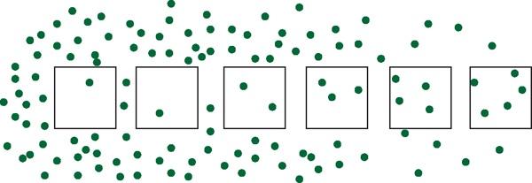
One transect might not be enough because you may miss a wider pattern (Figure 1.1). You ought to place several transects and combine the data from them all. In this way you are covering a wider part of the habitat and being more representative of the whole, which is the point.
Figure 1.1 One transect may not be enough to see the true pattern. In this case several transects would give a truer representation.
You also need to determine how long the transect should be. You might, for example, be looking at a change in abundance of a plant species along a transect, which may relate to an environmental factor. You need to make sure that you make the transect long enough to cover the change in abundance but not so long that you over-run too far.
Mixed sampling
There are occasions where you may wish to use a combination of systematic and random sampling. In essence, what you do is set up several transects and sample at random intervals along them. Think for example of a field where you wish to determine the height of some plant species. You could set up random co-ordinates but once you get to each co-ordinate how do you select the plant to measure? One option would be to measure the height of the plant nearest the top left corner. Each quadrat is placed randomly but you have a system to pick which plant to measure. You’ve eliminated bias because you determined this strategy before you started. Another option would be to place transects (a simple piece of string would do; the transect would then be a line transect) at intervals across the field. You then measure plants that touch the string (transect) or the nearest to the string, at some random distance along. There are many options of course and you must decide what seems best at the time. The point is that you are trying to eliminate bias and get the most representative sample you can.
Another example might be in sampling for freshwater invertebrates in a stream. You decide that you wish to look for differences between fast-running riffles and slow-moving pools. You need some systematic approach to get a balance between riffles and pools. On the other hand, you do not want to pick the “most likely” locations; you need an element of randomness. You might identify each pool and riffle and assign a number to each one, which you then select at randomfor sampling. Again the idea is to eliminate any element of bias.
Haphazard sampling
There are times when it is not easy to create an area for co-ordinate sampling, for example, you may be examining leaves on various trees or shrubs that have a “dark” and a “light” side. It is quite difficult to come up with a quadrat that balances in the foliage and you might attempt to grab leaves at random. Of course you can never be really random. In this case you say that the leaves were collected haphazardly. To further eliminate bias, you might grab branches haphazardly and then select the leaf nearest the end.
Whenever you get a situation where you stray from either a set system or truly random, you describe your collection method as haphazard.
1.6.5 Precision and accuracy
Whenever you measure something you use some appropriate device. For example, if you were looking at the size of water beetles in a pond you would use some kind of ruler. When you record your measurement, you are saying something about “how good” your recording device is. You might record beetle sizes as 2 cm, 2.3 cm or perhaps 2.36 cm. In the first instance you are implying that your ruler only measures to the nearest centimetre. In the second case you are saying that you can measure to the nearest millimetre. In the third case you are saying that your ruler can measure to 1/10th of a millimetre. If you were to write the first measurement as 2.0 cmthen you’d be saying that your beetle was between 1.9 and 2.1 cm.
What you are doing by recording your results in this way is setting the level of precision. If you used a different ruler you might get a slightly different result; for example, you could measure a beetle with two rulers and get 2.36 and 2.38 cm. The level of precision is the same
in both cases (0.01 cm) but they cannot both be correct (the problem may lie with the ruler or the operator). Imagine that the real size of the beetle was 2.35 cm. The first ruler is more accurate than the second ruler.
So precision is how fine the divisions on your scale of measurement are. Accuracy is how close to the real result your measurement actually is. Ideally you should select a level of precision that matches the equipment you have and the scale of the thing you are measuring. It seems a little pointless to measure the weight of an elephant to the nearest gramfor example.
1.7 Tools of the trade
Learning to use your spreadsheet is time well spent. It is important that you can manipulate data and produce summaries, including graphs. You’ll see a variety of aspects of data manipulation as well as the production of graphs later. Many statistical tests can be performed using a spreadsheet but there comes a point when it is better to use a dedicated computer program for the job. There are many on the market, some are cheap (or even free) and others are expensive. Some programs will interface with your spreadsheet and others are totally separate. Some programs are specific to certain types of analysis and others are more general.
Here you will focus on two programs. The spreadsheet you will see used is Microsoft Excel. This is common and widely available. There are alternatives and indeed the Open Office spreadsheet uses the same set of formulae and can be regarded as equivalent. The analytical programyou’ll see is called R; this is described first.
1.8 The R program
The program called R is a powerful environment for statistical computing and graphics. It is available free at the Comprehensive R Archive Network (CRAN) on the Internet. It is open source and available for all major operating systems.
R was developed from a commercial programming language called S. The original authors were called Robert and Ross so they called their programR as a sort of joke.
Because R is a programming language it can seem a bit daunting; you have to type in commands to get it to work; however, it does have a Graphical User Interface (GUI) to make things easier and it is not so different from typing formulae into Excel. You can also copy and paste text from other applications (e.g. word processors). So if you have a library of these commands, it is easy to pop in the ones you need for the task at hand.
R will cope with a huge variety of analyses and someone will have written a routine to perform nearly any type of calculation. R comes with a powerful set of routines built in at the start but there are some useful extra “packages” available on the CRAN website. These include routines for more specialized analyses covering many aspects of scientific research as well as other fields (e.g. economics).
There are many advantages in using R:
• It is free, always a consideration.
• It is open source; this means that many bugs are ironed out.
• It is extremely powerful and will handle very complex analyses as easily as simple ones.
• It will handle a wide variety of analyses. This is one of the most important features: you only need to know how to use R and you can do more or less any type of analysis; there is no need to learn several different (and expensive) programs.
• It uses simple text commands. At first this seems hard but it is actually quite easy. The upshot is that you can build up a library of commands and copy/paste them when you need them.
• Documentation. There is a wealth of help for R. The CRAN site itself hosts a lot of material but there are also other websites that provide examples and documentation. Simply adding CRAN to a web search command will bring up plenty of options.
1.8.1 Getting R
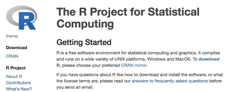
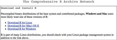
Getting R is easy via the Internet. The R Project website is a vast enterprise and has local mirror sites in many countries. The first step is to visit the main R Project webpage (http://www.r-project.org) where you can select the most local site to you (this speeds up the download process a bit).
Figure 1.2 Getting R from the R Project website. Click the download link and select the nearest mirror site.
Once you have clicked the download link (Figure 1.2), you have the chance to select a mirror site. These mirrors sites are hosted in servers across the world and using a local one will generally result in a speedier download.
Once you have selected a mirror site, you can click the link that relates to your operating system(Figure 1.3). If you use a Mac then you will go to a page where you can select the best option for you (there are versions for various flavours of OSX). If you use Windows then you will go to a Windows-specific page. If you are a Linux user then read the documentation; you generally install R through the terminal rather than via the web page.
Now the final step is to click the link and download the installer file, which will download in the usual manner according to the setup of your computer.
Figure 1.3 Getting R from the R Project website. You can select the version that is specific to your operating system.
1.8.2 Installing R
Once you have downloaded the install file, you need to run it to get R onto your computer. If you use a Mac you need to double-click the disk image file to mount the virtual disk. Then double-click the package file to install. If you use Windows, then you need to find the EXE file and run it. The installer will copy the relevant files and you will soon be ready to run R. Now R is ready to work for you. Launch R using the regular methods specific to your operating system. If you added a desktop icon or a quick launch button then you can use these or run R fromthe Applications or Windows Start button.
1.9 Excel
There are many versions of Excel and your computer may already have had a version installed when you purchased it. The basic functions that Excel uses have not changed for quite some while so even if your version is older than is described here, you should be able to carry out the same manipulations. You will mainly see Excel 2013 for Windows illustrated here. If you have purchased a copy of Excel (possibly as part of the Office suite) then you can install this following the instructions that came with your software. Generally, the defaults that come with the installation are fine although it can be useful to add extra options, especially the Analysis ToolPak, which you will see described next.
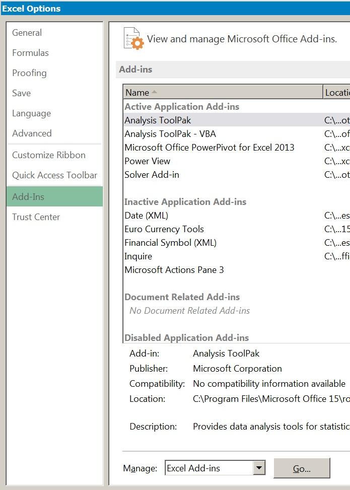
Figure 1.4 Selecting Excel add-ins fromthe Options menu.
1.9.1 Installing the Analysis ToolPak
The Analysis ToolPak is an add-in for Excel that allows various statistical analyses to be carried out without the need to use complicated formulae. The add-in is not installed as standard and you will need to set up the tool before you can use it. The add-ins are generally ready for installation once Excel is installed and you usually do not require the original disk.
In order to install the Analysis ToolPak (or any other add-in) you need to click the File button (at the top left of the screen) and select Options, then choose Add-Ins from the sidebar menu.
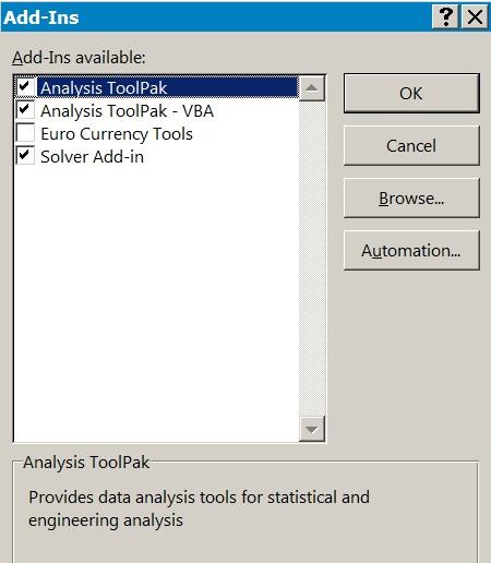
In Figure 1.4 you can see that there are several add-ins already active and some not yet ready. To activate (i.e. install) the add-in, you click the Go button at the bottom of the screen. You then select which add-ins you wish to activate (Figure 1.5).
Figure 1.5 Selecting the add-ins for Excel.
Once you have selected the add-ins to activate, you click the OK button to proceed. The addins are usually available to use immediately after this process.
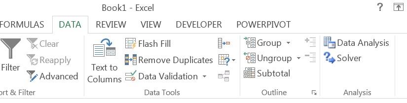
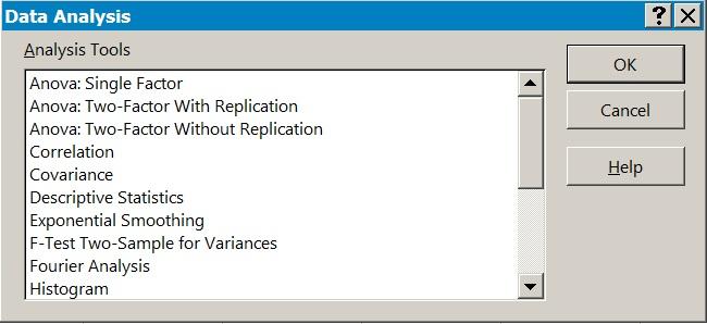
To use the Analysis ToolPak you use the Data button on the ribbon and select the Data Analysis button (Figure 1.6). Once you have selected this, you are presented with various analysis tools (Figure 1.7).
Figure 1.6 The Analysis ToolPak is available fromthe Data Analysis button on the Excel Data ribbon.
Figure 1.7 The Analysis ToolPak provides a range of analytical tools.
Each tool requires the data to be set out in a particular manner; help is available using the Help button.
1.9.2 Other spreadsheets
The Excel spreadsheet that comes as part of the Microsoft Office suite is not the only spreadsheet; of the others available, of particular note are the Open Office and Libre Office programs. These are available from www.openoffice.org and www.libreoffice.org and there are versions available for Windows, Mac and Linux.
Other spreadsheets generally use the same functions as Excel, so it is possible to use another program to produce the same result. Graphics will almost certainly be produced in a different manner to Excel. In this book you will see Excel graphics produced with version 2013 for Windows.
EXERCISES
Answers to exercises can be found in Appendix 1.
1. In a project looking for links between things you would be looking for or , depending on the kind of data.
2. Arrange these levels of measurement in increasing order of “sensitivity”: Ordinal, Interval, Categorical.
3. Domin, DAFOR and Braun-Blanquet are all examples of scales, whereas red, blue and yellow would be examples of .
4. Which one of the following is not a kind of transect?
A. Line. B. Belt.
Interrupted.
5. You select the most appropriate collection method to eliminate bias. TRUE or FALSE?
Chapter 1: Summary