About the Authors
Edward C. Weber has been in private practice as a radiologist for more than 30 years and has taught radiology to first- and second-year medical students at Indiana University School of Medicine in Fort Wayne (IUSM-FW) for almost 20 years. He guided the orientation of this book and provided most of the radiologic images and clinical information for it.
Joel A. Vilensky is an anatomist who has been teaching at IUSM-FW for more than 30 years. His role was primarily to ensure that all textual and graphic material presented in the book could be completely understood by students who have taken a course in medical anatomy and who have had some basic clinical experience.
Alysa M. Fog is a practicing PA who specializes in orthopedics. She ensured that the material was ideally presented for students and beginning medical professionals. Alysa also contributed much of the organization and clinical material for Chapter 2.
Contributors
Thanks to Peter Miller, MD; LCDR Kevin Preston, MD; and Keith Newbrough, MD for their generous contribution of images:
Peter Miller, MD, Indiana University School of Medicine
Chapter 1: Figure 1-3
Chapter 2: Figures 2-5, 2-12, 2-14, 2-28, 2-33, 2-36, 2-43, 2-47, 2-65, 2-67, 2-70, 2-76, 2-78
Chapter 3: Figures 3-3, 3-4, 3-5, 3-6, 3-7, 3-9, 3-11, 3-12, 3-28, 3-29
Chapter 4: Figures 4-1, 4-4, 4-5, 4-6, 4-7, 4-11, 4-13, 4-16, 4-18, 4-19, 4-20, 4-29, 4-33
Chapter 5: Figures 5-6, 5-13, 5-15, 5-17, 5-18, 5-19, 5-21, 5-22, 5-23, 5-24, 5-29, 5-30, 5-31, 5-33
Chapter 6: Figures 6-25, 6-43, 6-44
Chapter 8: Figures 8-1, 8-2, 8-3, 8-4, 8-6, 8-7, 8-9, 8-10, 8-11, 8-12, 8-13
Chapter 9: Figures 9-1, 9-2, 9-3, 9-4, 9-5, 9-10, 9-11, 9-17, 9-22, 9-24, 9-26, 9-27, 9-28, 9-29, 9-32
Chapter 10: Figures 10-15, 10-16, 10-17
LCDR Kevin Preston, MD, Indiana University School of Medicine
Chapter 2: Figures 2-35, 2-38, 2-39, 2-40, 2-41, 2-45, 2-56, 2-63, 2-79, 2-81, 2-83, 2-84
Chapter 6: Figures 6-5, 6-7, 6-12, 6-14, 6-18, 6-19, 6-21, 6-22, 6-23
Chapter 8: Figures 8-18, 8-20
Keith Newbrough, MD, Indiana University School of Medicine
Chapter 2: Figures 2-8, 2-9, 2-18, 2-29
Chapter 6: Figure 6-17
Chapter 7: Figure 7-5
Reviewers
Linda G. Allison, MD, MPH
Associate Professor, Pharmacy Practice
Belmont University School of Pharmacy
Nashville, Tennessee
Jesse A. Coale, PA-C
Assistant Professor
Physician Assistant Studies
College of Science, Health & the Liberal Arts Philadelphia University Philadelphia, Pennsylvania
Randy Danielsen, PhD, PA-C
Senior Vice-President
National Commission on Certification of Physician Assistants Foundation Johns Creek, Georgia
Steve B. Fisher, MHA, PA-C
Senior Surgical Physician Assistant
Department of Neurosurgery, Kentucky Neuroscience Institute University of Kentucky Lexington Kentucky
Charlene Morris, MPAS, PA-C, DFAAPA
Family Medicine
Pamlico Medical Center, PA Bayboro, North Carolina
1 MODALITIES OF MEDICAL IMAGING
RADIOGRAPHY
Radiography, discovered in 1895, is still the foundation of medical imaging. It is one type of imaging modality under the broader heading of radiology, which includes computed tomography (CT), magnetic resonance imaging (MRI), nuclear medicine (NM), and ultrasonography (sonography [US]).
Radiographic Densities
Radiography refers to the medical images that are the “shadows” projected onto a flat plane when x-rays pass through a patient. Similar to any shadow, they show the shape of the object causing the shadow. Figure 1-1 is a magnified small section of a chest radiograph. How many different anatomic structures do you see in this figure?
Surgical clips, bullet fragments, orthopedic hardware
and Associated Structures
Cortical bone; medullary bone is summation of bone density and marrow (fat, soft issue density)
The untrained eye and mind may only perceive several different structures. Careful and educated observation, however, reveals many more.
Radiographic shadows have different shades of gray that provide important information. These gray tones are referred to as radiographic densities. There are five radiographic densities, four biologic and one artificial/metallic density that is distinguishable from biologic calcium density (Table 1-1). You will see all four biologic densities if you look for them in Figure 1-1. It is normal to look at radiographs and just look at the shape of structures, but in order to fully comprehend the visual information in those images you must distinguish among radiographic densities.
The different shades of gray on a radiograph (radiographic densities) result from differences in the absorption and scattering of x-ray photons in their path from the x-ray source toward the digital x-ray detector. The degree to which x-rays are prevented from reaching the detector is referred to as radiographic attenuation. Different tissues attenuate the x-ray beam based upon the average atomic number and thickness of the tissue. These physical properties of tissue are also referred to as density, which can be confusing when radiographic density is often abbreviated as just “density.”
Calcified tissue attenuates more of the beam than fat or water because it has a higher average atomic number, and therefore calcified tissue has a higher radiographic density than fatty tissue or fluid. The final shade of gray that you see in any one location on a film or on a monitor reflects the attenuation of the x-ray beam by all of the tissues along the path of the x-ray beam to that part of the image. The summation density at any particular point on a radiographic image thus reflects both the density and thickness of the
Muscle, tendons, solid organs such as liver, fluidfilled structures such as gallbladder
Subcutaneous fat, intermuscular and other deeper fat planes
Any collection of air or gas such as lungs, loop of bowel
Radiographic and fluoroscopic images are sometimes shown as a “negative” of the standard representation given above, so that metallic objects are black and air density is white.
FIGURE 1-1 Magnified section of a PA chest radiograph.
TABLE 1-1 Radiographic Densities
intervening structures in the path of the x-ray beam at that anatomic position. There may of course be many overlapping structures that contribute to a particular summation density. Now look at Figure 1-2.
You may have noted the vertebral column initially (A in figure), but did you also notice the horizontal, very bright white lines representing the dense, compact bone of the vertebral body end-plates? These are brighter (more dense) than medullary bone in the remainder of the vertebral bodies. Medullary bone is not pure calcium density because marrow fat contributes to its summation density.
The first time that you looked at this figure, did you recognize correctly the border of the heart, or did you include epicardial fat as part of the heart shadow? Appreciating the lower radiographic density of epicardial fat allows you to accurately determine the border of the cardiac apex.
For an example of a summation density in Figure 1-2 look at the thick vertical band of very bright (white) density that is a summation density representing the descending aorta (B in figure) and other structures along the path of the x-ray beam. Note that the right side of the spine, visible through the heart shadow, is darker than the left side of the spine, visible through the heart shadow and the shadow of the aorta. You probably did not think, initially, that this image could show you the position or size of the descending aorta, but now you can ascertain that this patient has a normal leftsided aorta and it does not appear to be dilated.
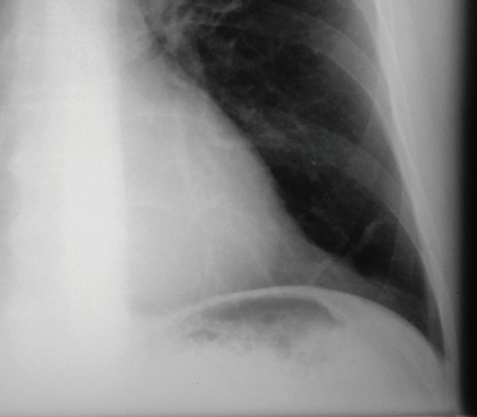
FIGURE 1-2 Same image as depicted in Figure 1-1 but labeled to highlight features visible if you look for subtle density differences. (A) Spine (calcium density); (B) Spine and aorta (calcium and soft tissue density); (C) arrow points to a disc space that is bordered by horizontal, very dense bone of vertebral endplates; (D) left border of spine and aorta; (E) right border of aorta; (F) right border of spine; (G) heart (soft tissue density); G2) muscle (soft tissue density); (H) fine dark stripe of intermuscular fat plane (fat density); (H2) epicardial fat pad (fat density); (J) lung (air density); (J2) air in gastric fundus (air density).
Untrained viewers just look at the shape of structures in radiographic images. However, by searching for subtle differences in radiographic density of different tissue, and appreciating summation densities, far more information can be discerned.
In later chapters, we will discuss the need for high quality radiography to show these shades of gray in specific clinical situations. Poor radiographs may fail to show important density differences. Even when radiographs are satisfactory, clinically important information that is visible may be overlooked if subtle differences in radiographic densities are not appreciated. For example, knee radiographs may not show a fracture but should not be interpreted as “negative” if the normal fat density deep to the quadriceps tendon is replaced by soft tissue or water density, perhaps indicating blood within the knee joint.
The interpretation of a radiograph and every other type of diagnostic image is an active rather than a passive process. You must look for normal anatomic structures and for evidence of pathology. In looking for the large number of important findings that may appear on a medical image, you must develop a consistent and thorough search pattern.
In radiography (and in CT), any edge that appears in an image is an interface between tissues that have different degrees of attenuation of the x-ray beam, such as the interface between air and soft tissue. When there is a horizontal edge between air and fluid in any medical image, it is called an airfluidlevel. Identifying an air-fluid level on an image helps identify anatomic structures that contain air and fluid and the orientation or position of the patient when imaged. The search for abnormal air-fluid levels is often crucial in finding and in identifying pathology, such as the presence of gas and fluid (pus) in an abscess.
To improve the contrast resolution of an image, specific contrast materials (or “media” or “agents”) may be administered to the patient. Contrast materials have a higher radiographic density than air, fat, or soft tissue, resulting in the visibility of structures that may not be seen on images without their use. (See section on Contrast Enhancement.)
COST-EFFECTIVE MEDICINE
High quality radiographs and interpretation provide diagnostic information that may avoid the need for more expensive cross-sectional imaging and may be critical in avoiding missed diagnoses.
Types of Resolution
Resolution refers to the ability to perceive two adjacent objects or points as being separate. Within radiology, the term is subdivided into spatial, contrast, and temporalresolutions.
The value of “sharp” images—that is, images with high spatial resolution—is obvious. Contrast resolution allows the differentiation among types of tissue. A third type of resolution may also be important: temporal resolution, the ability to image a structure during a very narrow window of time. As we discuss techniques and imaging protocols used to acquire clinically useful information, all three types of image resolution may be addressed, often with discussion of the strengths and weaknesses of different imaging modalities for different kinds of resolution.
COST-EFFECTIVE MEDICINE
These fundamental issues of spatial, contrast, and temporal resolutions are important in all imaging modalities. This is not a “technical” matter, it is a clinical issue. Does “X” imaging procedure have the temporal resolution that you need for a patient whose breath holding ability is limited? Does “Y” imaging procedure have the spatial resolution needed to see a very fine fracture of bone cortex? Does “Z” imaging procedure have the tissue contrast resolution to tell you if a tissue is edematous, although its size and shape are unchanged? Doing the ideal imaging procedure initially is less expensive than when a suboptimal procedure needs to be followed with additional studies.
Radiographic Projections
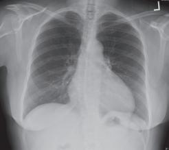
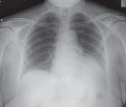
Note the apparent differences in the chest radiographs depicted in Figure 1-3. And yet they are the same patient! One cannot interpret radiographic images without understanding the various projections used.
Radiographic projections describe the relationship between the patient (body part) and the path of the x-ray beam. It is important to understand these projections in order to make sense of the anatomy shown and to understand why anatomic structures may appear differently in various projections.
PA/AP Views
In a PA projection, the path of the x-ray beam is from (the patient’s) posterior to anterior (Fig. 1-4, left). In an AP projection, the path of the x-ray beam is from (the patient’s) anterior to posterior (Fig. 1-4, right). Together, AP and PA projections are referred to as frontal views.
Because of the geometry of the diverging x-ray beam, anatomic structures may appear magnified, and this is often apparent when PA and AP projections are compared (Fig. 1-3). Those structures near the detector appear closer to true size than structures further from the detector (Fig. 1-4). The heart, an anterior structure in the thorax, is closer to the detector in the typical PA projection of an
FIGURE 1-3 PA and AP chest radiographs of the same patient. The top image is a standing PA chest radiograph; the bottom image is an AP upright chest radiograph done in an ED using a portable x-ray machine.
FIGURE 1-4 Diagram illustrating how PA and AP chest radiographs are done, with insets showing the relative representation of heart size on each.
upright patient and is thus more accurately depicted in a PA than in the AP projection (Figs. 1-3 and 1-4). In the portable AP radiograph shown in Figure 1-3, which was done on a semiupright patient in an emergency department (ED), the heart appears to be enlarged because of the geometric effect caused by the diverging beam.
Limitations of medical imaging, whether imposed by physics, imperfections of technology, or a variety of patient factors, such as metallic implants, and patient motion during imaging, can result in artifacts in a medical image. Countless times, a portable AP radiograph has been misinterpreted as showing cardiomegaly because of the geometric issue discussed above when in fact the heart was normal in size; therefore, never assume that a radiographic image perfectly represents “reality.”
Lateral Views
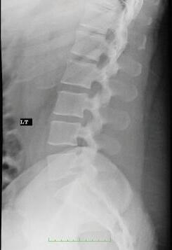
In a lateral projection the path of the x-ray beam is from one side of the patient or body part to the other side. You may hear the phrase “true lateral,” indicating that care was exercised in positioning the path of the x-ray beam in the coronal plane (Fig. 1-5). A “Left” or “Right” side marker is usually placed to indicate which side of the patient was closest to the detector. This is a different use of the markers than in frontal
or oblique projections, in which the markers indicate the right or left side of the patient.
Oblique Views
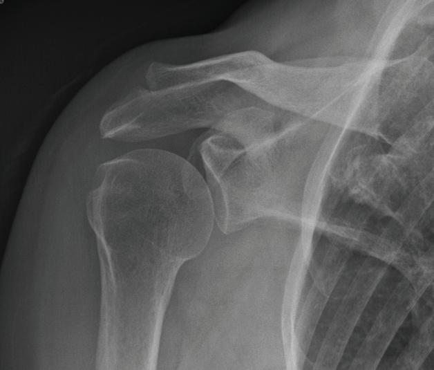
There are many oblique projections that demonstrate anatomic features more clearly than in frontal or lateral projections. The designation of an oblique projection is based upon the orientation of the patient relative to the path of the x-ray beam. For example, for a right posterior oblique (RPO) projection, one may start with the patient oriented for an AP projection and then rotate the patient so that his or her right side is closer to the detector than the left side. It is understood that the x-ray beam passed from the left anterior aspect of the patient toward the right posterior aspect of the patient.
Figure 1-6 is an example of a common posterior oblique projection of the shoulder, described by Grashey
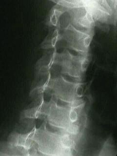
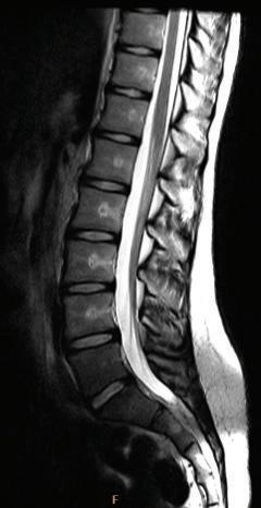
FIGURE 1-5 Left lateral radiograph of the lumbar spine. In lateral views the side indicator (LT) indicates the patient’s side closest to the x-ray detector.
30º
FIGURE 1-6 Grashey (oblique shoulder) view radiograph (top) and a schematic drawing of patient orientation for the Grashey view (bottom).
in 1923, used for ideal visualization of the glenohumeral joint.
In Figure 1-6, the patient is rotated to his right in relation to the x-ray beam. The most important issue when viewing oblique images is that there is no uncertainty about which anatomic structures are on the right side of the patient and which are on the left side. In other words, if an oblique projection of the cervical spine clearly reveals cervical neuroforamina, the important issue is that there must be certainty as to whether these are the right or left neuroforamina. It does not matter if the oblique view was done as a right posterior oblique or a left anterior oblique, as long as an “R” marker indicates to the viewer which side of the image is the right side of the patient or an “L” marker indicates the left side of the patient.
Oblique radiographic projections may not only be angled in a left-to-right (or mediolateral) direction. There are also numerous special projections that use cranio-caudal (or its opposite) angulation, and in some cases an angle that is oblique in two planes. However, many of the numerous special radiographic projections, often done with highly creative patient positioning, are now performed rarely, if at all, because cross-sectional imaging has becomes the procedure of choice for viewing abnormalities that formerly presented a great challenge to demonstrate radiographically.
COST-EFFECTIVE MEDICINE
Good radiography including proper use of oblique and other special radiographic views can sometimes obviate the need for more expensive procedures. You will provide the best patient care if you use the simplest, safest, and least expensive medical imaging, such as radiography and ultrasonography (or no imaging), as appropriate to establish a diagnosis.
Viewing Radiographic Projections
The traditional practice of viewing radiographs is simple and consistent: For almost every body part, except those listed in the next paragraph, the radiograph is viewed as if the patient is looking at you. This is true for any AP, PA, or oblique projection.
The exceptions are these: Hands, wrists, and feet are viewed as if you are looking at your own. Forearms may be viewed either as if the patient is looking at you with elbows extended (anatomic position) or you are looking at your own forearms.
Examples of the first rule can be found by looking at Figure 1-3. These were done differently, one AP and the other PA, but both are printed the same way. The patient’s left is to the viewer’s right. The patient is looking at you.
Another example is the oblique view of a right shoulder (Fig. 1-6; Grashey view). Imagine that this patient was facing you and then turned toward his right but can still look at you out of the corner of his eye. An oblique view may be obtained in different ways, but that does not change how it is viewed (Fig. 1-7).
This standardized method of displaying radiographic images provides a consistency of anatomic identification and recognition that is essential to minimize confusion and error. It is the expectation that every radiographic image be properly marked with a Left or Right indicator to avoid a potentially serious error such as trying to drain fluid from the right hemithorax when it is the patient’s left hemithorax that requires drainage. However, in the real world, the side markers may not be clearly seen, may be absent, or may be misplaced. In an emergency situation it is critical to have instant appreciation of which side of the patient has an emergent condition, rather than needing to search for the “R” or “L” identifiers.
The reason for standard image display that is independent from image acquisition can be explained through the following example: Imagine a patient is admitted to the ED and a portable AP chest radiograph is obtained. The next day, the patient is capable of standing for a PA chest radiograph. The patient’s condition then worsens, and a portable AP chest radiograph is again obtained, this time in the intensive care unit (ICU). When evaluating this series of images and looking for changing or new radiographic findings, imagine viewing the series of images if they were viewed from the perspective of how they were done, rather than in a standard presentation. An abnormal pulmonary density might be in the side of the image toward the viewer’s left in the first image, the right on the second image, and then back again toward the left. With multiple radiographic findings, viewing such a series of images would be very confusing.
A consistent appreciation of the patient’s side of a radiologic finding (e.g., which knee is arthritic on bilateral knee radiographs) is far more important when viewing radiographs than how a radiograph was done (AP or PA).
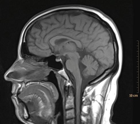
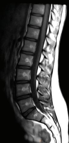
The presentation of lateral views is more complex and less consistent than the other projections. A traditional practice has been to orient lateral radiographs to match the position of the patient when the radiograph was made. An alternate practice that provides a more consistent viewing experience when radiographs are viewed with cross-sectional images is to match the common presentation of sagittal CT and MRI images (Fig 1-8). These are, almost universally, shown as if the anterior aspect of the patient is to the viewer’s left. This varies from the traditional practice of viewing sagittal ultrasound images, discussed later.
Topviewofpatient
Left anterior obliqueprojection
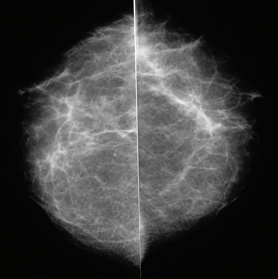
Mammography presents an interesting issue with respect to how the images are shown. The original standard was for the images to be shown as mirror images with the anterior aspect of the right breast toward the viewer’s left, and vice versa (Fig. 1-9). However, this standard is not consistently used among radiology practices.
Exceptions to standard radiology practices of viewing radiographs have always been common “in the clinic,” often for logical reasons. For example, because at one time almost all spinal surgery involved a posterior approach, many spine surgeons viewed AP and PA spine films as if the patient was looking away from them—that is, they were looking at the back of the patient and the patient’s right was to the viewer’s right. The rationale for viewing spine radiographs this way has lessened with the increase in anterior approaches in spine surgery. Furthermore, such a practice results in left-right orientation of radiographs that are opposite that of CT and
FIGURE 1-7 Illustration of how right posterior oblique and left anterior oblique projections are done. The figure shows that the resulting radiographic images are viewed the same way—as if the patient was (obliquely) facing the viewer.
FIGURE 1-8 Sagittal MRI of the head and brain. Sagittal cross-sectional images, by convention, are presented as if the patient is facing the viewer’s left.
FIGURE 1-9 Normal cranio-caudal (CC) mammographic views; the anterior aspect of the right breast is typically toward the viewer’s left and vice versa, but this is not always the case; thus, labeling of the right and left breasts is essential in mammograms. The lateral aspect of each breast is at the top of the image.
MRI, which are often viewed along with those radiographs. Consistency of image orientation reduces the chance of error.
CROSS-SECTIONAL IMAGING, TOMOGRAPHY, AND BODY PLANES
It has always been a challenge to differentiate anatomic features shown within various patterns on radiographs because of the projection of “shadows” of overlapping anatomic structures. Overlapping results in the summation densities discussed earlier. By the middle of the twentieth century, an advanced radiographic technique called tomography was in widespread use to improve visualization of specific anatomic structures in radiographic images. Standard radiographic tomography is a technique that blurs out features in front of and behind an anatomic plane of clinical interest by linear motion of the x-ray tube and detector (in opposite directions) during the exposure; only structures in the focal plane appear sharp.
Thus, tomography could be considered a cross-sectional imaging technique because it clearly showed the structures in only one section or slice of the body. Cross-sectional imaging today, whether CT, MRI or ultrasound, similarly reveals slices or sections of the body. Originally, CT only showed axial (transverse) sections of the body. Subsequently, software was developed enabling sagittal, coronal, and oblique sections to be depicted (Fig. 1-10).
MRI was a multiplanar cross-sectional imaging technique from its first clinical use. Ultrasound examinations are a handheld technique that can display cross-sectional images in any plane.
Modern cross-sectional imaging has revolutionized medical diagnosis through the clear visualization of internal
FIGURE 1-10 Anatomic planes. Purple, coronal; pink, sagittal; green, transverse (axial); orange, oblique. Cross-sectional images may be done in these conventional orthogonal anatomic planes here but may also be oriented in non-conventional multiple oblique planes.
anatomy. But as with radiography, cross-sectional imaging involves making compromises and is subject to false positive and false negative results. These will be discussed with the individual cross-sectional imaging techniques.
COMPUTED TOMOGRAPHY: CROSS-SECTIONAL IMAGES AND RECONSTRUCTIONS
CT is an advanced computer-based form of tomography in which cross-sectional images are produced from the mathematical analysis of a large number of measurements. Through several generations of CT equipment, different arrangements and movements of x-ray tubes and detectors were developed. During each rotation of the x-ray tube and detector array, measurements of the attenuation of x-rays at millions of locations and angles in the axial plane are acquired (Fig. 1-11). The specific levels of gray used for each pixel of a displayed CT scan have a numerical value (Hounsfield number) ranging from –1,000 to +1,000, in which air is –1,000, water is 0, and compact bone is +1,000.
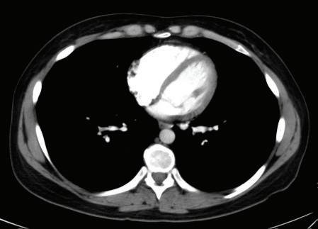
influence the duration of the scan, radiation exposure, and quality of the images. Furthermore, a large number of different image reconstructions are possible. The specific reconstruction algorithms used may be critical in determining what can be seen on the images. For example, the apparent density of an anatomic structure seen on CT can be misleading. Thicker reconstructed slices may have some advantages but may lead to an artifact called partial volume averaging, which results because each pixel (picture element) on the computer screen represents a voxel (volume element) of tissue (Fig. 1-12).
If a thickly reconstructed slice includes tissues of different CT densities, the apparent Hounsfield density measurement will be an average of all these tissues, and not an accurate measurement of any one of the individual anatomic structures included (partial volume averaging). A classic example would be the pulmonary nodule. A 5 mm thick slice that includes a 3 mm nodule and some normal lung tissue will not truly represent the density of the nodule.


Initially CT scanners were only able to acquire one axial section while the patient was motionless on a table, and then the patient table moved for each additional axial section, and so forth. More recent technology has resulted in the development of helical (spiral) scanners in which the patient table continuously moves during the CT scan. The most recent advance was the introduction of multidetector scanners that could acquire CT data from more than one slice simultaneously during each rotation of the x-ray tube and detector array. The first multidetector CT (MDCT) scanners were dual slice scanners. Progress has been rapid with the development of an increasing slice number on newer scanners. At this time, 64 slice scanners are common and the newest generation of scanners can image 256 or 320 slices in a single rotation. In addition, rotation speed has increased to where these many slices can be obtained in approximately 1/3 of a second.
Inherent to the process of CT image acquisition are variables that must be set by the operator of the unit and that
Depending upon the relationship between visualized structures and the orientation of a cross-sectional image, geometric shapes of anatomic structures may be distorted. For example, as shown in Figure 1-13, a round tubular structure that runs obliquely to the long axis of the body will appear as an oval structure on a conventional axial scan. Additionally, a structure such as the splenic vein that meanders cranially and caudally as it traverses from the spleen in the extreme upper left abdominal quadrant to the portal vein in the upper right quadrant may pass into and out of a specific image section and might be misinterpreted as separate structures when viewed in a single slice. This is why radiologists must review a number of adjacent sections, and view CT scans in multiple planes, in order to be absolutely certain they are identifying an anatomic structure correctly.
You might be surprised to know that the spatial resolution (sharpness) of CT images is often not as good as that available in conventional radiography. But the contrast resolution for soft tissues is much better in CT.
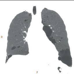
Subsequent to the development of helical CT scanning, continued software and computer development resulted in the ability to reformat the CT image data so that sagittal, coronal, and oblique CT images could be viewed. Special image displays, such as maximum intensity projections (MIP; Fig. 1-14) and minimum intensity projections (MinIP; Fig. 1-15) are used to improve visualization of pathology. Very life-like three-dimensional representations (volume rendered or 3D displays) of anatomic regions or structures may also be produced (Fig. 1-16).
Because CT is a procedure that relies on ionizing radiation, the same intravenous (IV) iodinated contrast materials that are used in conventional radiography may be used in CT.
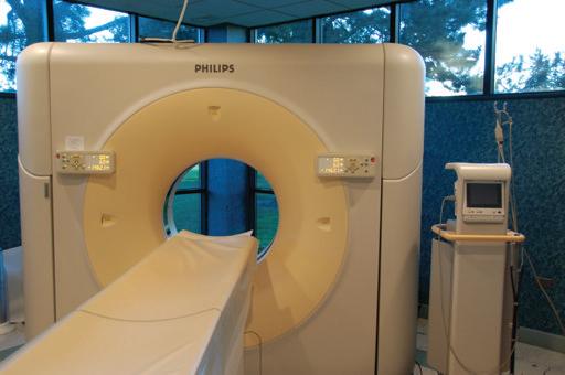
FIGURE 1-11 Illustration of basic CT scanner mechanisms with a photograph of a CT scanner.
FIGURE 1-12 Partial volume averaging. Voxel (volume element) of tissue is represented as a pixel (picture element) on a computer screen (A and B) and how a CT or MR slice (C) that is thicker (acquired thickness or displayed thickness) than a structure of interest (e.g., tumor) may not accurately represent the tissue density or signal intensity on the 2D image (note differences in gray color in the lower two images) because of the averaging of all the tissue within the voxel that are represented by the pixel (D)
The kinetics of the distribution of these agents must be considered when protocols are set up for contrast-enhanced CT studies. Thus, there are very specific protocols for contrast injection rates and timing between contrast injections and scanning for the imaging of various body regions. Another


FIGURE 1-13 Schematic illustration of geometric distortion and/or possible misinterpretations in cross-sectional imaging. “Monitors” show projected axial images. (A) An axial “slice” may show only a small section of a tubular structure that meanders cranially and caudally. (B) Two sections of the same structure could give the false impression that the two are entirely different structures. (C) Cross-section of one end of a tubular structure. Note that the other end is not in the lowest slice so that a radiologist may have to follow such structure in serial images “down” and then back “up” again. (D) A rectangular structure in cross-section appears to be a square structure. (E) The round cross-section of a tubular structure appears as round only if the structure is perpendicular to the slice, while if the structure runs obliquely to the image slice, it appears as an ovoid structure.
protocol issue relative to CT is the exposure to radiation. A typical CT scan exposes a patient to significantly more radiation than a standard radiographic study. But it should be noted that the exposure in a typical CT exam is about a third of the radiation a person receives from background radiation in a year. Nevertheless, as a primary care provider you need to be aware of patient radiation exposure concerns, especially if the patient is subjected to multiple CT scans or if the patient is a child (see Patient Safety section later in this chapter).
Axial CT images are presented as if the viewer is standing at the foot of the patient’s bed; the patient’s right is to viewer’s left; the anterior aspect of the patient is toward the top of the image (Fig. 1-17). Coronal images are viewed the same way that the majority of radiographs are viewed; the images are oriented as though the patient is looking at you (Fig. 1-18).
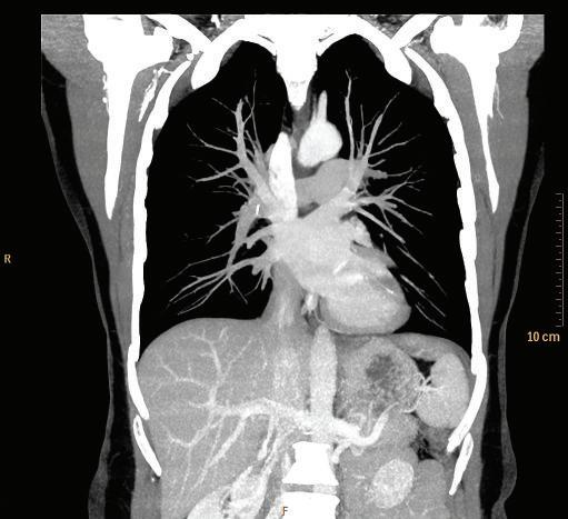
FIGURE 1-14 Coronal maximum intensity projection (MIP) of a chest CT.
Sagittal CT images are shown as though the patient is looking toward the viewer’s left (Fig. 1-19).
CT is capable of capturing a much greater range of radiographic densities than can be appreciated by our visual system, which typically can differentiate about 16 shades of gray.
MRI also captures more than 16 levels of tissue signal intensity. Therefore, decisions must be made for the mapping of CT density levels and MR signal levels to the gray-scale values on an image used for viewing. These choices are referred to as windowing and leveling.
Because windowing and leveling in CT is a more important and clearly ordered process than in MRI, the following discussion will focus on CT. However, a similar process is followed when viewing MR scans.
The CT window is the range of densities that will be compressed into the shades of gray for viewing. In a narrow window CT image, only the CT densities within a limited range are assigned to various shades of gray, with tissues that have a CT density below that range depicted as black and tissue above that range depicted as white. The CT level refers to the mid density of the window. Narrow window CT images are perceived as high contrast, or very black and white, images. These images make conspicuous very slight differences in CT density among tissues but depict little contrast resolution for tissues outside the range chosen. A wide window CT image assigns broad
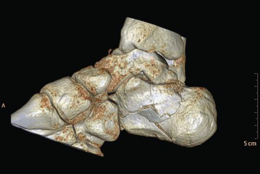
FIGURE 1-16 Three-dimensional volume-rendered display (CT) of the hindfoot showing multiple fractures of the calcaneus (red arrowheads).
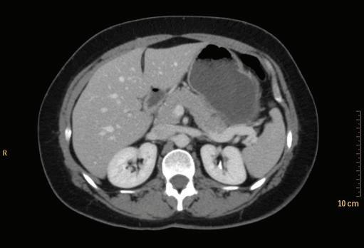
FIGURE 1-17 Axial CT of the abdomen.
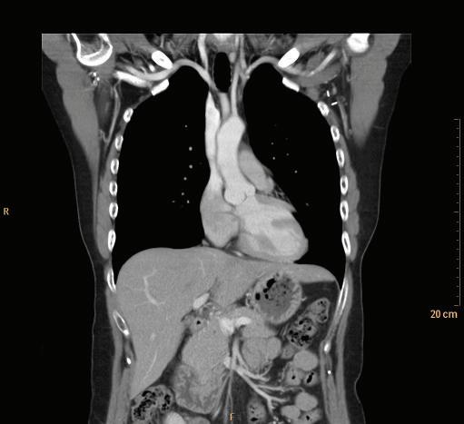
FIGURE 1-18 Coronal CT of the chest.
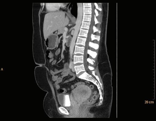
FIGURE 1-19 Sagittal CT of the abdomen.
FIGURE 1-15 Coronal minimum intensity projection (MinIP) of a chest CT.
ranges of CT density to each visible shade of gray but is perceived as a very low contrast, or very gray, image (Fig. 1-20).
MAGNETIC RESONANCE IMAGING
MRI does not involve patient exposure to ionizing radiation. MRI is based on the principle that protons may emit radio
waves in the presence of strong magnetic fields and pulses of radiofrequency energy, neither of which have been shown to have significant biologic effects. Each set of images is the result of a series of radiofrequency pulses and variations in the magnetic field, known as a “pulse sequence.” The physics of MRI is very complex and only a simplified description is provided here.
A typical MRI scanner looks grossly like a larger and thicker CT scanner (Fig. 1-21). Some MRI scanners, however, have different configurations, such as those open at the sides or vertically oriented. These “open” and “vertical” scanners may have some advantages for the claustrophobic patient but also may acquire images more slowly and may have reduced image quality compared with the closed scanners.
MRI scanners are often described by the strength of their primary magnet, typically 1.5 Tesla (unit of magnetic field strength). The primary magnetic field is modified by additional magnetic fields, resulting in varied magnetic field strengths or “gradients” that are used in the production of images. These fields affect the “spin” of hydrogen protons within the patient’s body. Radiofrequency pulses are applied to these protons, which then emit radio waves (not that different from those received by your car radio) that are detected by antennas, called receiver coils. The output from those coils is used to create cross-sectional images. The specific gradient fields and radio pulses chosen for each set of images (known as a “pulse sequence”) not only result in cross-sectional images in any chosen plane but also in the different appearance of tissues on the images.
The pulse sequences used in clinical MRI are quite varied, the most common of which are T1 or T2 spin echo, T1 or T2 fast spin echo, or T1 or T2* gradient echo sequences, as well as commonly used FLAIR and STIR sequences. Proprietary names for many pulse sequences available on MR scanners from different manufacturers are often referred to on radiology reports. However, sequences are often just referred to as either T1 or T2 sequences (or T1-weighted or T2-weighted) sequences.
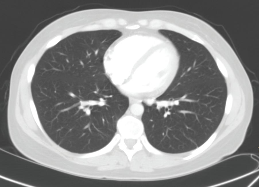
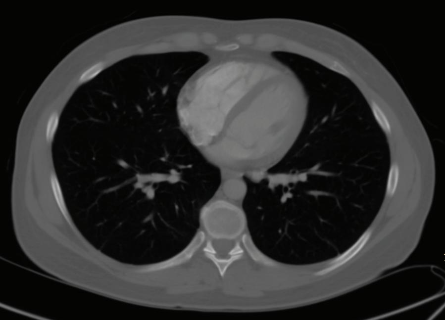
FIGURE 1-20 Three axial chest CT images using different window settings. The top image was made using a soft tissue window. In this image, the different soft tissue densities (note: muscles and intermuscular fat planes) and the bright contrast enhancement of blood in the heart are very conspicuous. The middle image was made using a lung window setting, in which lung markings, mainly pulmonary veins, are visible. The lower image was made using a bone window setting. With these window and level settings, you can see the distinction between marrow and cortical bone in the ribs.
FIGURE 1-21 Photograph of a magnetic resonance (MR) scanner.
In T1 image sequences, fluid has low signal and appears dark on the image. Lipids and other specific tissues may have high signal and be bright (T1 hyperintensity). With contrast enhancement by a gadolinium-based contrast agent, tissue that contains the agent has high signal on T1-weighted images. In T2-weighted images, fluids (or tissue with high water content) have a high signal and appear bright (T2 hyperintensity) (Fig. 1-22 and Table 1.2). PD (proton density) sequences are neither T1 nor T2 weighted.
There are both T1 and T2 sequences that use a variety of techniques to suppress the MR signal from lipid, so that high signal from a lipid-containing tissue does not obscure high signal from adjacent high signal fluid or a gadolinium-enhanced tissue. These are referred to as fat suppressed (“FS”) sequences.
MRI has intrinsically better soft tissue contrast resolution than CT. For that reason, there are many imaging examinations, such as internal derangement of the knee, in which MRI is vastly superior to CT. In other situations in which
FIGURE 1-22 T1-weighted and T2-weighted axial MR lumbar spine images. Note that the cerebrospinal fluid (CSF) is hyperintense (bright) in T2 image and hypointense (dark) in T1 image.
TABLE 1-2 Comparison of the Typical Appearance of Tissues on T1 and T2 MR Images*
Tissue TypeT1-Weighted ImagesT2-Weighted Images
FluidDarkBright
AirBlackBlack
MuscleIntermediateIntermediate to dark
TendonVery darkVery dark
Bone cortexBlackBlack
Bone marrowBrightIntermediate to bright
FatVery brightIntermediate to bright
GadoliniumBright to very brightNo change from non-contrast (dark in high concentrations)
*Dark means low signal intensity, shown on images as darker shades of gray or black; bright means high signal intensity, shown on images as lighter shades of gray or white; intermediate signal intensity is assigned to an intermediate shade of gray on images.
either MRI or CT would be equally appropriate for diagnostic evaluation, but in which intravenous contrast administration (either iodinated- or gadolinium-based) is contraindicated by issues such as renal failure, unenhanced MRI is usually superior to unenhanced CT.
Because of the very strong magnetic fields associated with MRI, most metal objects should be removed from the patient before he or she enters the MRI room. Any other object that could also be affected by the magnet, such as credit cards, should also be removed. For surgically implanted (or otherwise embedded) metallic devices and objects, the issue becomes quite complicated, both with respect to safety and reduced image quality (because of the effect of such metal on the magnetic field). Do not make the assumption that because your patient has such an implanted metallic device he or she cannot undergo MRI. It depends upon the metals used, the shape of the objects, and the specific anatomic location involved. Many patients are given cards for their devices pertaining to MRI safety. Consult with the imaging facility you are referring the patient to in order to determine whether the patient can undergo MRI. A valuable resource to use is the web site www.MRIsafety.com.
MRI is an expensive diagnostic modality and may be difficult for the patient to undergo for psychological reasons, most notably claustrophobia. It has very high contrast resolution but is not the ideal imaging modality for every case. For example, compact bone has little or no MRI signal and therefore CT is better than MRI for cortical bone. The presentation of axial, sagittal, and coronal MR images is the same as in CT.
ULTRASOUND
Ultrasound was first developed for medical diagnostics in the middle of the twentieth century. In ultrasound, high frequency sound waves (1 to 30 MHz) are produced by a transducer, usually in contact with the skin. Pulses of sound waves are reflected back (echoed) to the transducer at interfaces between and within body tissues. Using an estimate of the speed of sound, the ultrasound unit places a dot (typically white) on the monitor screen at the locations that represent the positions from which each echo occurred. These dots create a cross-sectional image of the anatomy at the projected plane of the transducer on the body (Fig. 1-23).
A fluid-filled structure that contains no debris, precipitate, or cells will not have any interfaces within it to reflect sound. The fluid will be anechoic; on the image there will not be any echoes within a homogenous fluid collection. The echogenicity (level of gray or brightness on an ultrasound image) of soft tissue is described in relation to other tissues. Tissue that has the same echogenicity as the predominate