DYNAMIC TENSEGRITY SYSTEMS
MSc Dissertation - 2009 -10
Emergent Technologies and Design (EMTECH)
Architectural Association School of Architecture, LONDON
DISHITA TURAKHIA
ARCHITECTURAL ASSOCIATION SCHOOL OF ARCHITECTURE
GRADUATE SCHOOL PROGRAMMES
COVERSHEET FOR COURSE SUBMISSION 2009/2010
PROGRAMME:Emergent Technologies and Design
TERM:Autumn 2010
STUDENT NAME: Dishita Turakhia
SUBMISSION TITLE: MSc Dissertation | Dynamic Tensegrity Systems
COURSE TUTOR: Mike Weinstock
SUBMISSION DATE:15/10/2010
DECLARATION:
“I certify that this piece of work is entirely my own and that any quotation or paraphrase from the published or unpublished work of others is duly acknowledged.”
SIGNATURE OF STUDENT:
DATE: 15/10/2010
ACKNOWLEDGEMENTS
First and foremost, I am extremely grateful to our Emtech course director, Michael Weinstock for his tremendous encouragement, guidance, support and inspiration through out the one year of course study. I would also like to thank George Jeronimidis and Toni Kotnik for their immense support and much valued feedback at every stage of the project development. I also would like to thank course tutor Christina Doumpio ti for her effort and time devoted in helping the project take shape. I would also like to thank all the AA Emtech Staff, my colleagues and class-mates for everything that I was able to learn while working with and around them.
I can never thank enough my parents, Girish Turakhia and Meena Turakhia for their forever encouraging support and all their love and belief in me that constantly inspires me at every stage of my work. I would like to acknowledge the support and efforts of my group mate and dear friend Riddhi for all the help and assistance o ffered. Lastly, I want to thank all my family and friends both here and back home who have always been my suppor ting pillars.
03
ABSTRACT
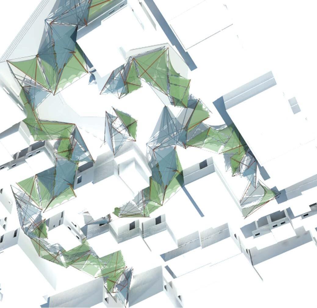
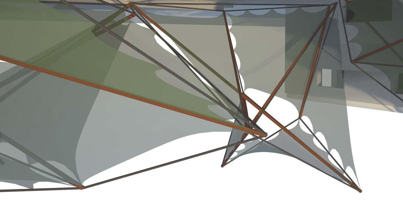
The research intends to develop Dynamic Tensegrity Structures for designing programmatically driven habitable structures in a highly dense and mixed use urban context. The primary purpose of the ‘dynamic’ nature of the system proposal is to serve the rising needs for flexibility, adaptability and mul ti-func tionality of space, due to lack of expansion of land in congested site contexts. Thus the resultant reconfigured structure would provide for optimal spatial use as per the user needs at various time scales. The research aims at providing a feasible solution to the considered contextual situation by addressing the various limitations of the system development- namely computational, analy tical and fabrication.
05
6
For ever-expanding megaci ties, rapid changing social context is an area of major concern for architectural structures. With shi fts in lifestyles and social condi tions, the land-use pattern of the city is undergoing a major transition continuously. Advancing economies and occupations result in periodically re-diagrammed urban map of the city with overgrowing satellite towns enveloping the main city thus increasing the loads on energy consumption and infrastructure.
For congested ci ties, that lack any further urban space for expansion and any further resources to support the infrastructure, it is essential to design multi-use structures that are programmatically adaptive spaces. These essentially can be small scale adaptive structures for rehabilitating the low-cost social communi ties which transform into economy generating spaces like house-hold factories and manufacturing units by day and residential housing units for the families by night. Another possibility for adaptive infrastructural structures is public health and learning centers by day and social congregational and recreational spaces by night. These adaptive temporary structures can also be highly useful for disasterbased rapid rehabilitation spaces.
The proposed design case, however, attempts at addressing the issue of lack of flexible and mul ti-use adaptive habitable spaces in densely populated urban contexts with a continuous influx of varied social groups. This concern is addressed essentially by developing dynamically configured Tensegrity Structures. The project further investigates the
various organization strategies of the designed Tensegrity modules evolved using algorithmic design process. The organization logic reflects the juxtaposi tion of existing spatial condi tions and required re-configured enclosed spaces, both of which are listed following a thorough study and analysis of site condi tions at varied time scales.
The further investigation involves understanding change connec tion parameters of the components and the respective resultant alteration in the spatial nature of the design. The process followed for developing these Tensegrity modules involves generative algorithmic approach to produce highly varied morphologies within a limited set of principles and parameters, followed by an intensive evaluative analysis and elimination procedure to filter out the most optimized and useful modules. The strength and stability of the design system is tested digitally using material properties and constraints in analy tical so ftwares like Strand in order to understand the load bearing capacity and buckling thresholds for the design.
The resultant filtered morphologies selected based on structural and spatial quali ties are further organized within the selected context of over-crowded, congested and ever-expanding city of Mumbai. The final design proposal addresses the construc tion and installation techniques from a critical view-point to be able to propose a viable design solu tion to the addressed problem in the chosen context.
7
INTRODUCTION
8
SYSTEM
PROCESS
DESIGN (TENSEGRITY) (DYNAMIC TENSEGRITY) (MUMBAI SLUMS)
ARCHITECTURAL
CASE STUDIES
BIOMIMETIC
FORM FINDING
ROBOTICS
DIGITAL (PARAMETRIC)
EXPLORATION
EVALUATION
PHYSICAL
GEOMETRY GENERATION
RELAXATION TO STABLE FORM
VOLUME
HEIGHT
BASE AREA
STRUT INTERSECTIONS
COMPONENT SIZE
REGULAR
CLASSIFICATION
DYNAMISM + MULTIPLICITY
IRREGULAR
ROTATIONAL
TELESCOPIC
EVOLVING URBAN CONTEXT
TYPES OF USES AND USERS
SETTLEMENT TYPOLOGIES
TIME-LINE OF CHANGE
MATERIAL AND DETAIL
DESIGN APPLICATION
FABRICATION AND INSTALLING
SYSTEM BEHAVIOUR
DESIGN DEVELOPMENT
INTEGRATED PROPOSAL
9
DIAGRAM
10
CHAPTER 1 DOMAIN
Introduc tion
Case Studies
Conclusion
CHAPTER 2 METHODS
Introduc tion
Key Concepts
Case Studies
CHAPTER 3 EXPERIMENTS
Preliminary Exploration
Generative Algorithm
Structural Tests
CHAPTER 4 DESIGN DEVELOPMENT
Spatial Exploration
Mul tiplicity
Membranes
Module Organization
CHAPTER 5 DESIGN PROPOSAL
Revised Design Strategy
Site
Time-line Study
Organization Strategy
Test Proposal
Construc tion Details
CHAPTER 6 CONCLUSIONS
Learnings
Limitations
Further Scope
APPENDIX
REFERENCES
11
CONTENTS
13 14 19 27 29 30 34 42 47 48 54 64 69 70 72 76 79 81 82 83 86 88 90 94 101 102 103 104 107 171
12
CHAPTER 01.
DOMAIN
01 INTRODUCTION
Need For Flexibility in Architecture
State of Art Examples
Tensegrity: Tool for Flexibility
02 CASE STUDIES
BioTensegrity - Dynamic Models of Tensegrity in Nature
Architectural Applications of Tensegrity
03 CONCLUSION
This chapter aims at developing the argument and theoretical base for the research project concluding to the primary intention and hypothesis of the dissertation. The introductory sec tion focuses on cri tically addressing the di fferent concerns and aspects of the study and the explored premises of the respective concepts. The case studies focus on studying the existing examples of the system application in both natural and architectural contexts. The conclusion sec tion further reiterates the thesis intent and design concern based on the case studies and analysis.
13
INTRODUCTION
NEED FOR FLEXIBILITY IN ARCHITECTURE
Amidst rapidly changing social contexts, architectural structures require distributed intelligence embedded in ac tive material systems, programmable virtual representations of themselves (digital models) that are capable of changing their internal parameter and performances in relation to the life of the inhabitants and events in the external world [1.1]
This need for Socio-Spatial Response arises from the new way of lifestyles reflecting not only the mobility and speed of modern life but also its temporary nature and potential of expandability. Cedric Price, quite ambitiously explores the potential of this concept by stating “What if the buildings or a space could be constantly generated and regenerated!” [1.2]
This intriguing fascination of dynamic structures is also described by Neil Leach in his essay[1.3] wherein he states “in most advanced form, it would be an architecture that is open to those processes themselves, an
adaptive, responsive environment, that does not crystallize into a single, inflexible form, but is able to recon figure itself over time, and adjust to the multiple permutations of programma tic use that might be expected of it”.
Using dynamism to improve efficiency, multi-func tionality and adaptability of space has become a design pre-requisite in order to cater to the rising need of domestic flexibility. Of all the architectural programs, this dire need of design adaptability is most evident in residential spaces. “A home cannot be defined by its functions but is a pa ttern of regular activities and neither the space nor its appurtenances have to be fixed. A home is an organiza tion of space that has some strcture in time, in which people interact in a pa ttern of events and phenomena that integrate space and performance. ”[1.4] With increasingly changing lifestyles and advancement
14
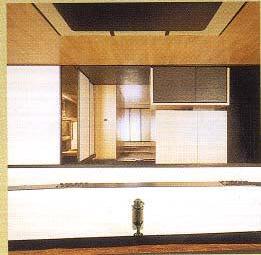
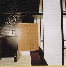
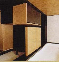
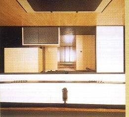
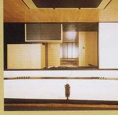
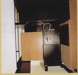
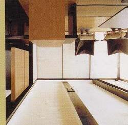
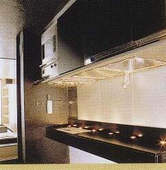
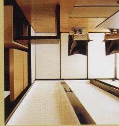
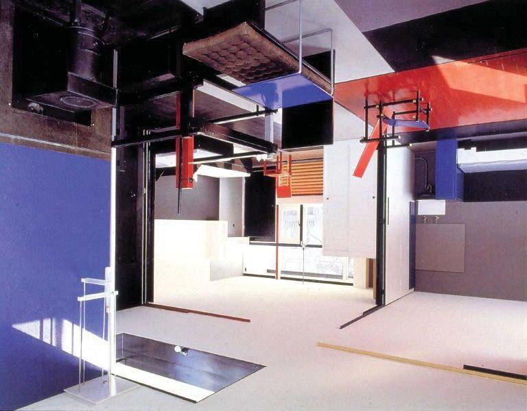
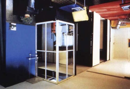
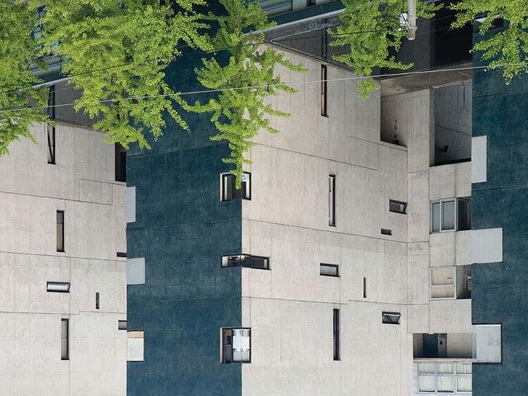
FIG 1.1. Images showing different combinations and configurations of internal arrangements and use of hinged partitions in the Fukuoka Housing in Japan by Steven Holl

in technological connec tivity, the lines and needs for conventional func tionally demarcated spaces is rapidly diminishing. Tradi tional notions of family units are being exploded as it fractures into small groupings, dispersed in the urban landscape. With constantly changing equations between space user and spatial use in this rapidly evolving age, there is a need for a house or living space to have the potential of variability, reconfigurability and personalization based on user needs and requirements. This concept of adapting to the dynamic context is also discussed by Richard Rogers; he says, “Shelters will no longer be sta tic objects but dynamic objects sheltering and enhancing human events. Accommodation will be responsive, ever-changing and ever-adjusting.” [1.5] This need is further gravely realized in highly dense and congested urban contexts where lack of expansion space results in overlapping of programs within limited spaces. This results in mul ti-use of a given space and need for program based adaptability of the space and structures.
The further investigation briefly studies the various concepts, theories and designs exploring dynamic spatial re-configuration at varied scales and time spans.
References:
1.1 Adam Somali - Fischer, Interactive Architecture, Architectural Design - 4D Space
1.2 Cedric Price, Interactive Architecture, AD 4-D Space
1.3 Neil Leach, Swarm Techtonics, Digital Techtonics
1.4 Gillian Crampton Smith, Interactive Architecture, 4D Space.
1.5 Robert Kronenburg, Transportable Environments (1997), pg 45.
FIG 1.1. Transportable Environments (1997), pg 50.
FIG 1.2 http://solardecathlon.cca.edu/?p=78
15
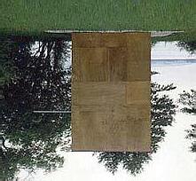
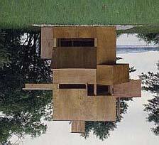
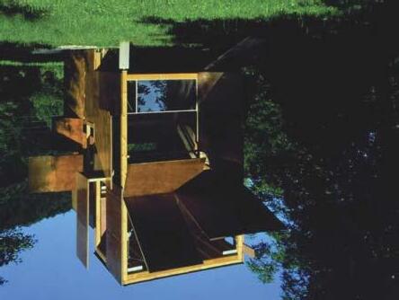
FIG 1.2. Series of different structural & spatial configurations in the GucklHupf by HansPeter Wörndl showing dynamic change of spaces.
STATE
ART
The concept of transformation and flexibility in domestic space has been explored widely and extensively over a long time since the beginning of twentieth century. The Schröder House[1.6] designed by Gerrit Rietveld (1924) was one the ground breaking realization of a transformable adaptive and flexible domestic design, having a system of sliding par titions that helped in achieving an extremely flexible interior arrangement almost on a daily basis. On the other hand, Buckminster Fuller’s 4D Dymaxion house(1927)[1.7], made of Duralumin explored a completely di fferent concept of efficient dynamism with deployable housing unit prototype for low-cost mass produc tion based on techniques drawn from aircraft and vehicle industries. Steven Holl’s no tion of ‘hinged space’ being most dynamic, interactive and movable and thus being the epitome of the transformable is exempli fied in his built housing project for Fukuoka
in Japan(1989)[1.8], with rooms designed with removable corners and rotating walls. While most of the flexibility explorations of a house are conventionally deemed to be in its floor plan, Iain Borden[1.9] describes the potential of transformations of domestic spaces vertically by exploring vertical circulatory elements. Yet another signi ficant model of kinetic structure is the GucklHupf by HansPeter Wörndl(1993)[1.10], exploring and experimenting the no tion of house reac ting with its environment through structure and skin, by disintegrating from its cocoon-like form and opening up into its surrounding.
These paradigms in architecture explore this concept of flexibility at varied scales of architecture and time from being daily internally reconfigurable to having this concept explored at an long time spanned external level. The primary intention of this brief case study was to grasp and extract these application methods and apply at an altogether di fferent scale
16
OF
FIG 1.3. Images showing different combinations of internal arrangements in the living space and sitting room of the Schroder House designed by Gerrit Rietveld
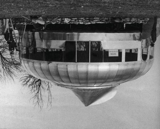
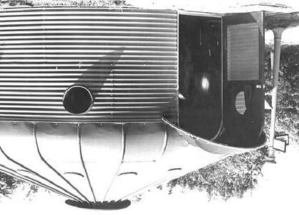
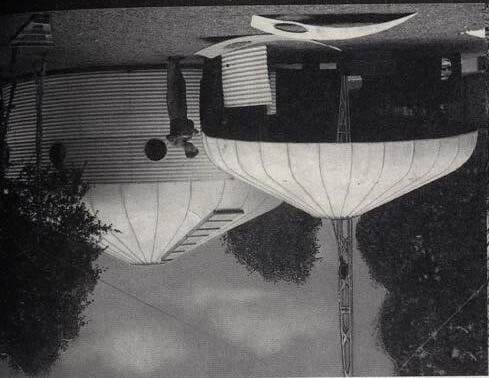
1.4. Different versions and designs of the deployable Dymaxion House designed by Buckminster Fuller for low-cost mass housing.
of structural level. The research aspires to address and develop the no tion of structural re-configurability resul ting from varying program needs of the space and user.
References:
1.6 Huber-Jan Henket, The Reitfeld-Schroder House (AD, The Transformable House) (2000), pg 12-15
1.7 Dennis Sharp, Maximum Deployment in a Dymaxion World (AD, The Transformable House) (2000), pg 16
1.8 Steven Holl, Hinged Space (AD, The Transformable House) (2000), pg 50
1.9 Iain Borden, Stairway: Transforming Architecture in the Golden Lane (AD, The Transformable House) (2000), pg 20
1.10 Sally Godwin, Hans Peter Worndl: The Glucklhupf (AD, The Transformable House) (2000), pg 86
FIG 1.3. http://static.rnw.nl/migratie/www.radionetherlands.nl/features/cultureandhistory/rietveld001214
FIG 1.4. http://www.sustainy.com/?p=675
FIG 1.5. http://aedesign.wordpress.com/author/alfredomaldonado2009/
1.5. Flexible & transformable external facade of the Fukuoka Housing Complex in Japan designed by Steven Holl.
17
FIG
FIG
a lightweight lattice of interlocking icosahedrons and could be skinned with a protective cover.
TENSEGRITY IN ARCHITECTURE
With most of the flexibility arising as a result of interior reconfigurations or skin variation, there is evidently little exploration in structurally dynamic adaptability potential of a building. Since, a space is embedded in its structure that is typically static[1.11]; it is essential to approach the design by developing a structurally flexible and reconfigurable system to achieve the spatial and func tional variation. In order to attain this flexible structural system that responds to user based spatial needs, the system needed to be not only morphologically varied and temporary but extremely strong and instantly reactive to certain key parameters. Tensegrity systems display all these characteristics and hence the research
aims at addressing the flexible design concern by exploring the potential of Tensegrity structures and applying in the varying programmatic urban context. With feasibility of this exploration being the primary concern and limitation of the Tensegrity System owning to its temporary nature, the research aims at addressing various other limitations like lack of ease of fabrication and on-site installation in the considered urban context. The research also questions the limited architectural exploration of Tensegrity Structures restricted to either sculptures or temporary tents in spite of the huge scope of varied applications.
References:
1.11 Klien Dytham, Interactive Architecture, Architectural Design - 4D Space FIG 1.6 http://www.arkinet.com/articles/agenda-the-bucky-bar-opens-tonight
18
FIG 1.6. Geodesic Tensegrity Installation to a habitable scale proposed by Buckminster Fuller as dome that deploy
01 BIOMIMETIC (BIO-TENSEGRITIES)
Anatomical Level
Cellular Level
Molecular Level
02 ARCHITECTURAL
Sculptures
Bridges
Installations
In order to study proper ties, characteristics, applications and potential uses of Tensegrity Structural System, it was essential to cri tically analyze the existing examples of this system. The primary goal of this exercise was to extract logics of processes and optimally applying these concepts for design development.
19
CASE STUDIES
BIO-TENSEGRITY
BIOMIMETIC EXAMPLES: Dynamic Tensegrity Structures in Nature
Biological models essentially provide for a coherent case study for understanding dynamic open systems.[1.12] Complex collec tive behavior of a dynamic system generally emerges from interactions among components that exhibit simple behavior. Tensegrity systems too, like other complex systems are widely existent in nature exhibi ting dynamic mechanisms in processes at various scales from anatomical level to cellular level and molecular level. It is important to study these examples not only for a better investigation of the system but also to understand the dynamic behavior of these systems as most of the Tensegrity natural systems display locomo tive or kinetic mechanisms. Since the basic aim of the research focuses on Dynamic Tensegrity Structures, it is crucial to study natural mechanisms that display dynamic proper ties in optimal way.
References: 1.12 Donald Ingber
FIG 1.7. http://www.magicalrobot.org/BeingHuman/2010/04/introduction-to-biotensegrity
http://www.ttem.org/forum/index.php?topic=1807.0
20
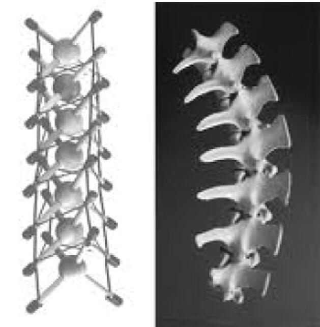
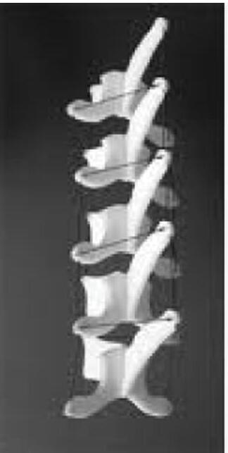
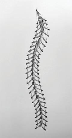
FIG 1.7. Tensegrity analogy models of Human Vertebrate column.
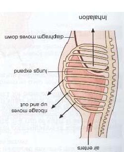
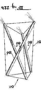
FIG 1.8. Diagram of 8 strut Octa-hedral Tensegrity model depicting the expansion and contraction mechanism of ribcage during respiration
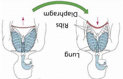
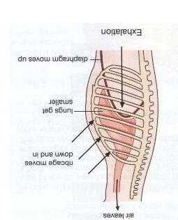
1.9. Images showing expansion and contraction of rib-cage and diaphragm during respiratory process.
ANATOMICAL EXAMPLES
On an anatomical level, the human body provides a good example of a prestressed Tensegrity structure. Bones act as struts resisting the pull of tensile muscles, tendons and ligaments. Moreover, the stability of the shape of the body, or its stiffness, of the body is a func tion of the tone, or prestress, of its muscles. As Ingber puts it, “We are 206 compressionresistant bones that are pulled up against the force of gravity and stabilized through a connec tion with a continuous series of tensile tendons, muscles, and ligaments”. [1.13]
Core Body Torso
The core of the body, the torso has bilateral symmetry, oscillates (breathes) and is bounded on all sides by bony structures. Breathing causes the thoracic cage to expand and contract following the pumping action of the diaphragm. By abstracting the shape somewhat it is feasible to map the force vectors of the torso onto an expanded octahedron Tensegrity. The diagram alongside shows a Modi fied X-Octa Tensegrity, which contracts
and expands in the same way the torso does, and there is a central cavity, as found in the body, created by the geometry. As two parallel struts are pulled apart (equivalent to the expansion of the ribs) both other parallel pairs counter intui tively expand and pull away from each other as well. Built from only six struts (suitably modi fied) they correspond to the boundary planes of the torso– the transverse planes of the clavicle and the pelvis, the coronal planes of the spine and sternum, and the sagi ttal planes of the ribs on both sides. [1.14]
The study of this bio-tensegrity demonstrates uniform dynamic volumetric changes resulting with mere changes in tension of the cables.
References:
1.13 Donald Ingber, How cells (might) sense microgravity
1.14 Donald Ingber, How cells (might) sense microgravity
FIG 1.9. http://www.oum.ox.ac.uk/thezone/animals/life/respire.htm
21
FIG
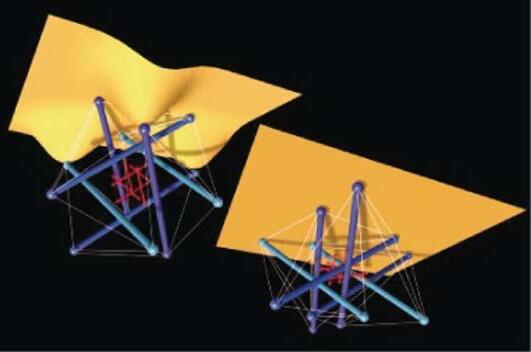
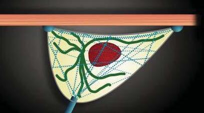
CELLULAR LEVEL EXAMPLES:
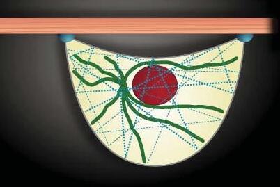
The cell possesses a molecular framework called the cytoskeleton enclosed within the surface membrane that mechanically stabilizes the cell. The cytoskeleton is comprised of three di fferent types of molecular protein polymers, called micro filaments, intermediate filaments and microtubules. This network of molecular struts and cables allows the cell to alter the balance of tension and compression throughout its structure in order to maintain its shape, even when external forces are imposed upon it.
Cytoskeleton:
The cellular Tensegrity model proposes that the whole cell is a prestressed Tensegrity structure, wherein tensional forces are borne by cytoskeletal microfilaments and intermediate filaments, and these forces are balanced by interconnected structural elements that resist compression, most notably, internal microtubule struts and extracellular matrix
(ECM) adhesions. The tensional prestress that stabilizes the whole cell is generated actively by the contractile actomyosin apparatus. Although the simple six-strut Tensegrity model of the cell has been very useful, the living cell is more complex because it is a ‘mul ti modular’ Tensegrity structure. The cell is composed of mul tiple smaller, self-stabilizing Tensegrity modules that are linked by similar rules of tensional integrity. As long as these modules are linked by tensional integrity, then the entire system exhibits mechanical coupling throughout and an intrinsic harmonic coupling between part and whole. However, destruction of one unit in a mul ti-modular Tensegrity, however, results only in a local response; that par ticular module will collapse without compromising the rest of the structure.
References:
FIG 1.10 http://www-3.unipv.it/webbio/anatcomp/freitas/2007-2008/biocell_LSBUSB07-08.htm
FIG 1.11 http://jcs.biologists.org/cgi/content/full/116/7/1155
FIG 1.12 http://jcs.biologists.org/cgi/content/full/116/7/1157
22
FIG 1.10. Diagrammatic representation of cytoskeleton expansion and contraction stages with Tensegrity concept.
FIG 1.11. Multi-modular model of Tensegrity organization of cytoskeleton that enables dynamic behavior.
FIG 1.12. Multi-modular hierarchical organization and composition of Tensegrity modules.

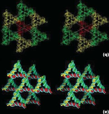
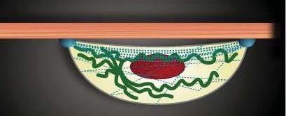
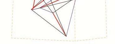
1.15. The stereoscopic images showing the surroundings of one triangle (a) and the rhombohedron flanked by eight of the triangles (b). The red triangle is at the back of the rhombohedron.
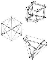
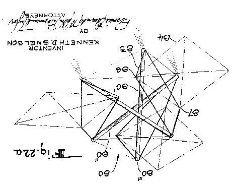
MOLECULAR LEVEL EXAMPLES:
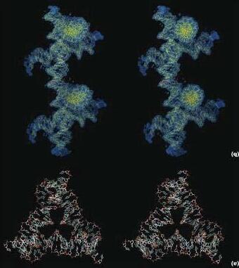
Several geodesic Tensegrity structures naturally occur on the molecular level. Basement membrane proteins, polyhedral enzyme complexes, clatrin-coated transport vehicles, viral capsides, lipid micelles, individual proteins, and RNA and DNA molecules all employ hexagonal arrangements.
DNA MOLECULE
Prof. Nadrian C. Seeman constructs stick figures of DNA where specific
sticky ends are attached to DNA branched junc tions, whose edges are double-stranded DNA. This approach has already been used to assemble a cube, a truncated octahedron , nanomechanical devices and 2-D crystals and 3-D crystals from DNA. This method of construc tion was originally stimulated by Seeman’s desire to characterize Holliday junc tions. Holliday junc tions are four-arm branched DNA molecules that are found to be structural intermediates in genetic recombination. In the last few
years, the symmetry, crossover topology and sequence-dependent thermodynamics of Holliday junc tions have been characterized and analyzed.
References:
FIG 1.13. http://www.dreamstime.com/3d-dna-model-image2260749
FIG 1.14. http://tensegrity.wikispaces.com/DNA
FIG 1.15. http://tensegrity.wikispaces.com/DNA
23
FIG 1.14. The stereoscopic images showing the molecular structure of the tensegrity triangle (a) and the connection between two of them through a sticky end (b).
FIG 1.13. DNA Molecule Diagram
FIG
TENSEGRITY IN ARCHITECTURE
KENETH SNELSON SCULPTURES:
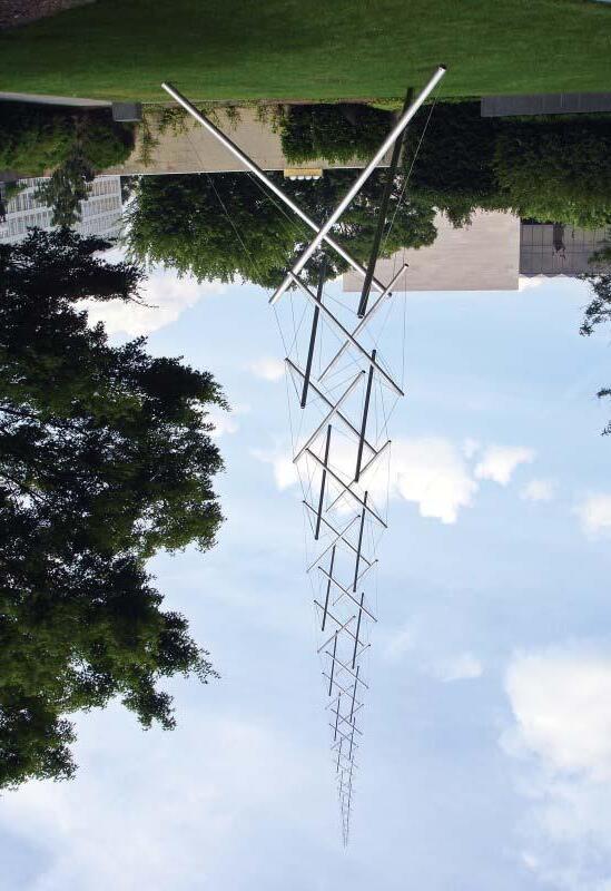
Needle Tower:
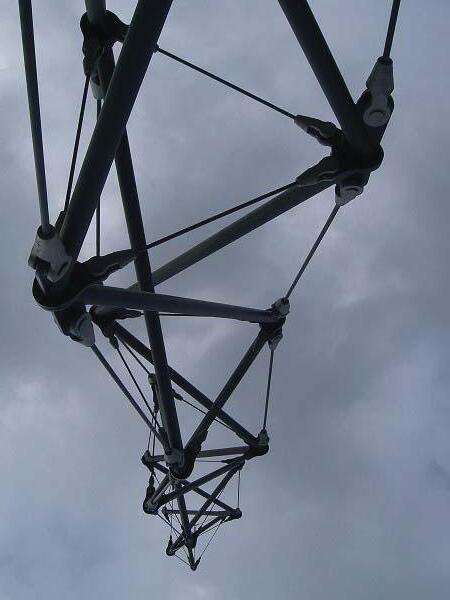
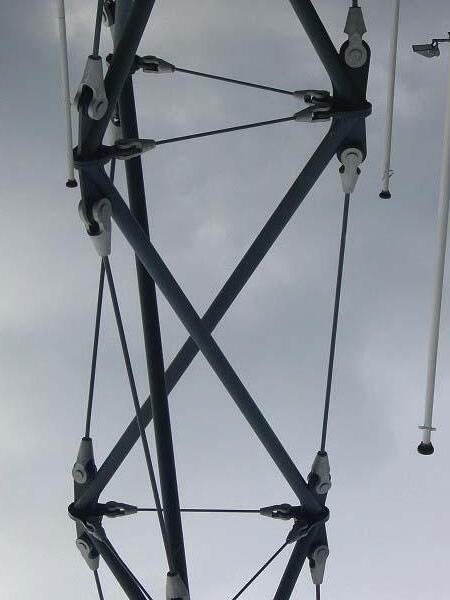
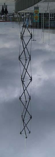
The needle tower was built by Kenneth Snelson in 1968 at the Hirshhorn Museum of Art. The structure was a succession of Tensegrity modules, decreasing in size, organized around a ver tical axis, very similar to the organization of the human spine.
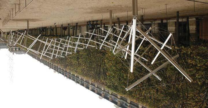
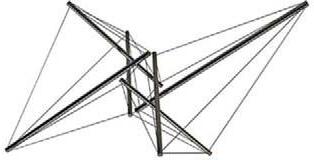
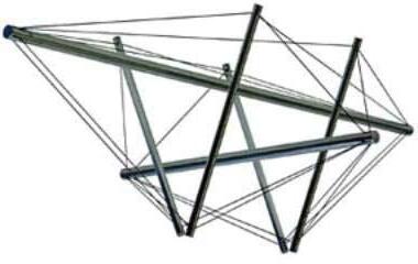
The Dragon:
A cantilevered Tensegrity structure built in 2000, wherein the forces of gravity are balanced in the structure by the tensile continuum of forces. The stresses that arise in the lower parts of the cantilever are distributed to the whole structure, allowing large cantilevers.
References:
FIG 1.16. http://kennethsnelson.net/1970/needle-tower/ FIG 1.17. http://www.brooklynrail.org/2009/04/art
24
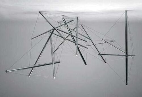
FIG 1.16. Kenneth Snelson’s Needle Tower, 1968 made of Aluminum & stainless steel measuring 60 x 20 x 20 feet or 18.2 x 6 x 6m present at Hirshhorn Museum & Sculpture Garden, Washington, D.C
FIG 1.17. Kenneth Snelson’s Dragon Sculpture made of stainless steel measuring 30.5 x 31 x 12 feet or 9.3 x 9.4 x 3.6m
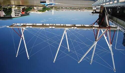
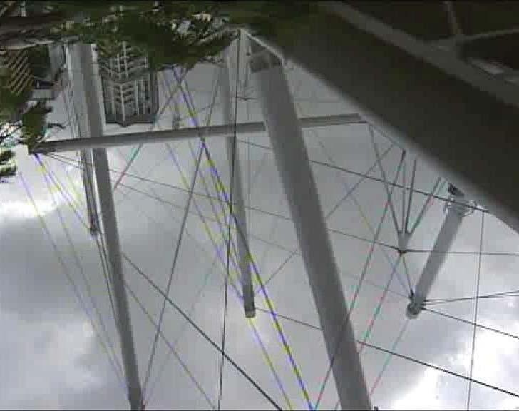
THE TANK STREET BRIDGE:
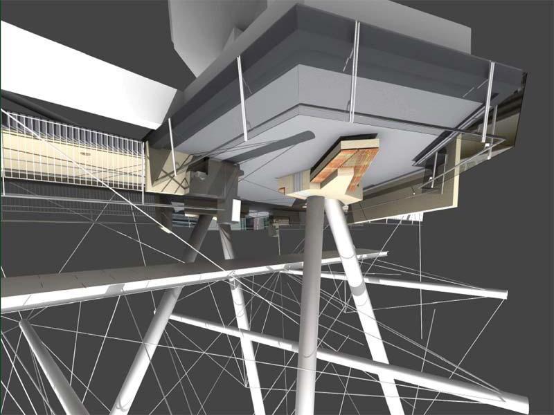
The tank Street Bridge is designed by Baulderstone Hornibrook Queensland and Cox Rayner Architects, in Brisbane Australia in collabora tion with ARUP. This bridge of 425m is the first Tensegrity Bridge for pedestrians and bicycles ever built solely as a Tensegrity structure. The bridge was built from both ends, without any supports since the Tensegrity property of the structure takes into account the gravity forces and thus allows large cantilevers.
References: http://www.archdaily.com/12914/tank-street-bridge-or-kurilpa-bridge-baulderstone-hornibrookqueensland-cox-rayner-architects/
FIG 1.18.http://www.archdaily.com/12914/
FIG 1.19. http://www.archdaily.com/wp-content/uploads/2009/01/1833331501
25
FIG 1.18. Image of The tank Street Bridge
FIG 1.19. Digital model of the connection end of the tank bridge
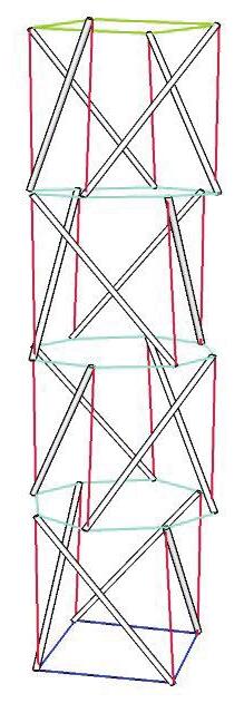
TENSEGRITY TOWER:
(Herbert Klimke, Soerren Stephan)
The Tensegrity Tower was conceived by architects Gerkan, marg and Partners for a fair in Rostock, Germany, in collaboration with engineers Schlaich, Bergermann and Partners. The modules of the tower consisted of three 10m long struts and nine cables. The produc tion method, fabrication technique and assembly logics followed in the project were extremely crucial and helpful in understanding the prac tical constraints and hindrances in the execu tion of a large Tensegrity Design project. The procedure was executed in 3 steps:
- Assembly of modules using temporary supports for posi tioning the struts
- Complete Pre-Stressing using three jacks of 100t capacity.
- State of interconnec tion of modules
References: 1.
1.20.http://www.del-uks.com/wiki/index.php/Nowhere_2007
FIG 1.21. http://www.mero.de/fileadmin/downloads/bausysteme/publikationen/tens_tower_e.pdf
FIG 1.22. http://www.mero.de/fileadmin/downloads/bausysteme/publikationen/tens_tower_e.pdf
26
FIG
FIG 1.20. Digital diagram of Tensegrity Tower showing modular organization
FIG 1.21. Detailed view of the Modular Connection of the Tensegrity Tower
FIG 1.22. Six tier modular Tensegrity Tower of three strut Tensegrity module
CONCLUSION
As per the research and case-studies, it can be observed that the high dynamic potential of the Tensegrity system has not be u tilized or even explored in the Architectural fields. The only applications of the System seen is for bridges, installations or sculptures. However, there is wide potential nd scope of developing this system into habitable structures and thus the research aims at achieving this goal of designing habitable and usable dynamic Tensegrity structures.
References: FIG 1.23.http://www.knowledgerush.com/kr/encyclopedia/Buckminster_Fuller/
27
CONCLUSION
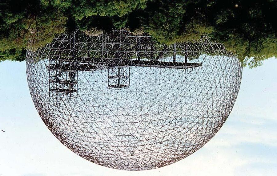
FIG 1.23 The American Pavilion of Expo ‘67, by R. Buckminster Fuller, now the Biosphère, on Île SainteHélène, Montreal
28
CHAPTER 02.
METHODS
01 INTRODUCTION
Non Linear Dynamic Systems
Tensegrity as Non Linear Dynamic System
Digital Methods and Tools
Simulation of Tensegrity Structures
02 KEY CONCEPTS
History
Defini tions
Characteristics
Advantages
Disadvantages
Classi fication
Theories and Methods
03 CASE STUDIES: Methods
Physical Exploration
Robo tics
Digital Locomo tion Simulation
Conclusion
This chapter focusses on setting up a theoretical base for need to develop system specific digital tools and processes in order to study, analyze, experiment and explore the complex system behavior. It then briefly summarizes the key concepts and characteristics of Tensegrity followed by case studies from parallel fields of research that focus on developing contemporary methods to explore dynamic system behavior.
29
INTRODUCTION

CAUSALITY PRINCIPLE
INPUT
Direct Relation and Proportion
STRICT CAUSALITY
Linear Systems OUTPUT
NON LINEAR DYNAMIC SYSTEMS
Manuel DeLanda, in his wri tings describes the signi ficant di fference between conventionally studied Linear Systems and the recently researched Non-linear complex system behaviors.[2.1] The Linear Systems tend to be characterized by a single global state, but the systems which are both non-linear and non-equilibrium display mul tiple stable states and these may come in a variety of addi tional forms, namely steady, periodic and chao tic states. These concepts are also explained by Causality Principle[2.2] which describes relationship between the causes and effects. A Strict Causality displays a predictable linear behavior with the result being directly propor tional to the input parameters; A Weak Causality also displays a fairly predictable yet imprecise behavior based on the input factors; Distributed Causality which is displayed by most of the non-linear dynamic systems wherein small variations of the ini tial condi tion of the system may produce large variations in the long term behavior of the system. These mul tiple stable states characterize not only
WEAK CAUSALITY
DISTRIBUTED CAUSALITY
Direct Relation
INPUTOUTPUT
INPUTOUTPUT
Unpredictable Relation and Proportion (Cause)(Effect) (Cause)(Effect) (Cause)(Effect)
Non-Linear Dynamic Systems
inorganic material behavior, but also organic social behavior.[2.3] “We are beginning to understand that any complex system, whether composed of interacting molecules, organic creatures or economic agents, is capable of spontaneously genera ting order and actively organizing itself into new structures and forms” , DeLanda says.[2.4] It is precisely this ability of matter and energy to self-organize and exist in mul tiple stable state, that is of greatest significance due to its potential application in various fields of design and development. The spontaneous generation of form as well as the morphogenetic potential of a material system can be best expressed by studying and analyzing its complex and variable behavior.
References:
2.1 Manuel DeLanda, Material Complexity, Digital Tectonics - (2004), pg 14
2.2 Heinz-Otto Peitgen, Hartmut Jurgens, Dietmar Saupe, Chaos and Fractals- (1992), pg11
2.3 Manuel DeLanda, Material Complexity, Digital Tectonics - (2004), pg 16
2.4 Manuel DeLanda, Material Complexity, Digital Tectonics - (2004), pg 15
FIG 2.1 http://www.citrinitas.com/history_of_viscom/computer.html
30
FIG 2.1 Illustration created in Processing which are the result of a non-linear physics-based model of keywords connected by springs.
BASIC SEED
RELAXED FORMS
TENSEGRITY AS NON LINEAR DYNAMIC SYSTEM
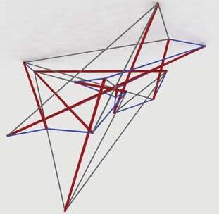
Although the conventionally studied classical Regular Tensegrity Structures can be classi fied as Linear Systems, the recent investigation in the field of developing and designing the Irregular Tensegrity has led to understanding the complex behavior of Irregular Structures.[2.5] While the primary parameters governing the morphological stable state of the system are the properties of its compressive and tensile components, the connection logic and nodal degrees kinetic freedom of the configuration also contribute signi ficantly to the resultant stability. These parameters essentially govern the Distributed Causality behavior of the system where a slight variation in the ini tial condi tions affect drastically the morphology of resultant varied stable state. Tensegrity structures, with its potential to configure itself into mul tiple stable states based on equilibrium states of its components, provides for a very efficient system to be explored for dynamic structural behaviors. Quite paradoxically, the kinematics of the system informs the static and final form of the configuration of the
system. The primary objec tive of studying Irregular Tensegrity Structures is to design a structurally dynamic Tensegrity system that inherently possesses a potential to adapt to the varying contexts and its respec tive demands, requirements and spatial needs.
References: 2.5 Manuel DeLanda, Material Complexity, Digital Tectonics - (2004), pg 14
31
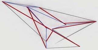
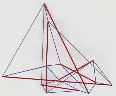
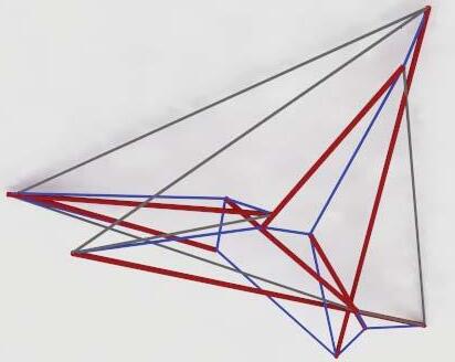
FIG 2.2 Diagram illustrating nonlinear behavior of Tensegrity System with multiple stable relaxed states existence from same unstable basic seed
DIGITAL TOOLS AND METHODS
SYSTEM
BEHAVIOR SIMULATION
DIGITAL METHODS AND TOOLS
One of the most challenging constraints in studying the behavior of a complex dynamic system is the tedious nature of the conventional analog methods that comprises of tradi tional physical testing and mathematical analysis procedures. This results in the need for developing advanced digital tools and processes that can cope with the complexity of the system behaviors without complicating the usability of the tool interface. Thus while on one hand, digital analy tical methods facilitate for studying material and structural system behavior, properties and characteristics for enabling in-depth understanding and precise prediction of the system performance under varied conditions; on the other hand, digital simulations facilitate for optimal solu tions and performance. Kristina Shea, in her essay “Directed Randomness” explains the importance of computational generative design and its use with instantaneous
SYSTEM BEHAVIOUR ANALYSIS
GENERATIVE DESIGN
Optimised Output
STRUCTURAL PERFORMANCE
feedback to generate new forms and design solutions with optimized space usage, structural performance, thermal conditions, lighting effects and fabrication ease. Use of structural shape grammar combined with simulated annealing so ftwares like eifForm, enable producing results with structural efficiency, economic material use, member uniformity, satisfied structural feasibility constraints combined with aesthetics. Exploring the potential of this methodology for formal, morphological and structural configurations and variations is one of the main areas of research of the intended study.
References: FIG 2.3 http://www.citrinitas.com/history_of_viscom/computer.html
32
FIG 2.3 Illustration created in Processing which are the result of a non-linear physics-based model of keywords connected by springs.
DIGITAL METHODS FOR TENSEGRITY:
Tensegrity Structural Systems constitutes 3-dimensional stable mechanical structures that maintain its stability due to an intricate equilibrium of forces established between its rigid and disjoint compressive and continuous tensile components. Tensegrity structures not only exhibit an exceptionally high strength-to-weight ratio but also possess the unique property of retaining its stability in zero-gravity spaces. However, the determination of stable configurations that result from the connec tivity patterns between the compressive and tensile components is highly challenging. Thus the form-finding processes of the Tensegrity structures involve computational support juxtaposed with algorithmic approach to overcome the limitations of the available mathematical methods that have restricted scope of exploration. This research involves use of Evolu tionary Algorithmic approach to thoroughly investigate a set of arbitrary Tensegrity Structures which are di fficult to design using tradi tional methods and
determine new irregular forms with optimal architectural relevance. The procedure involves use of Dynamic Relaxation methods for simulating the material properties and system performance to obtain stable forms based on the input mechanical constraints and kine tic freedom. The rigorous analysis, evaluation, elimination and selec tion procedure aims at achieving optimal set of digitally developed and tested modules provide for the basis for next stage of design development and complexity based on organization logics of the emergent design.
References:
2.5 John Rieffe , Automated discovery and optimization of large irregular tensegrity structures
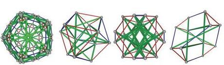
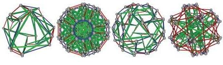
FIG 2.4 http://www.cabinetmagazine.org/issues/23/wertheim.php
33
FIG 2.4. Examples of symmetric tensegrity structures produced by Robert Connelly and Allen Back using Maple and the open source visualization software, Geomview.
This sec tion briefly summarizes chronologically the various investigations undertaken and the respective inferences concluded by different researchers and scientists on Tensegrity systems. While studying the defini tions enabled a deeper system understanding, the contemporary research methods helped in developing theoretical physics base for scripting the algorithmic form finding process during the dissertation project.
BACKGROUND
Until the last century, the technique of construc tion and the philosophy of building have been very simple with everything being held in place by weight, so the continui ties of stress were basically compressive. Tensegrity structures are based on a quite an inverse concept wherein instead of the “weight and support” strategy, a “system of equilibrated omni-direc tional
stresses” is integrated. Furthermore, the system need not be supported as it is self-equilibrated and pre-stressed, thus independent of gravitational forces for equilibrium.
Tensegrities are spatial, reticulated and lightweight structures that basically consist of isolated compression members (rigid bars) suspended by a continuous network of tension members (cables). These highly intriguing structures, especially for their unique visual quali ties and topological characteristics, were first developed by artist Kenneth Snelson in 1948 as well as independently by David Emmerich. Buckminster Fuller further developed Tensegrity structures from Snelson’s ideas by applying engineering principles to the study. He also coined the term Tensegrity from “tensile integrity” as the integrity or stability of the system comes from the tension members. As implied by their name, Tensegrity structures to dynamic loading and exhibit non-linear behavior.
34
HISTORY
FIG 2.4 Earlier explorations of Tensegrity structures progressing from 3-strut to 8 strut models
FIG 2.5 Sketches of Kenneth Snelson Experiments explaining forces in a 3-strut Tensegrity module
FIG 2.6 Diagram explaining analogy of Inflated and Pneumatic structures behaving like Tensegrity Systems.
DEFINITIONS

FIG 2.7 Diagram explaining basic forces and components forming a Tensegrity structure
COMPRESSIVE STRUTS
TENSILE CABLES
DEFINITIONS
-Buckminster Fuller(1961)
-David Emmerich
-Kenneth Snelson(1965)
-Anthony Pugh(1976)
-Schodeck(1993)
-Bin-Bing (1998)
-Kanchanasaratool& Williamson (2002)
-Ariel Hanaor
-Miura & Pallegrino(2002)
-Rene Motro(2003)
FIG 2.8 Diagram listing chronological research and respective researchers. Refer Appendix for detailed study listed.
DEFINITION:
Although Tensegrity System has been highly researched with varied patented defini tions, the most widely accepted and comprehensive defini tion can be summarised by Anthony Pugh’s (1976) explanation, “A tensegrity system is established when a set of discontinuous compressive components interacts with a set of continuous tensile components to define a stable volume in space.”
A brief description summarizing all the di fferent patented defini tions by the researchers who have explored and experimented varied aspects of Tensegrity Systems, is listed in the Appendix sec tion for further reference.
References: Darrell williamson, robert e. Skelton, and jeongheon han, tensegrity structures and their application to architecture chapter 4. Definitions and basic principles equilibrium condi tions of a tensegrity structure
FIG 2.3 http://www.citrinitas.com/history_of_viscom/computer.html
35
OF
CHRONOLOGY
RESEARCH
CHARACTERISTICS

SYSTEM:
TENSILE NODAL FORCES
COMPRESSIVE
NODAL FORCES
In relation to the theory of systems, it has components (two kinds, in compression and in tension), relational structure (between the different components), total structure (associating relational structure with characteristics of components) and form (projected on to a threedimensioned referenced system).
STABLE SELF EQUILIBRIUM STATE:
The system is stable because it can re-establish after a disturbance, and self-equilibrated because it doesn’t need any other external condi tion; it is independent of external forces (even gravity) or anchorages due to its self-stress ini tial state. It is stable even in orbit.
COMPONENTS:
In contrast to the term “element”, the component can be a strut, a cable, a membrane, an air volume, an assembly of elementary components,
etc. The components are either in compression or tension as opposed to component being in compression and tension. There is continuous tension and discontinuous compression in the system because the compressed components must be disconnected, and the tensioned components are creating an “ocean” of continuous tension.
FALSE AND PURE TENSEGRITIES:
Motro defines a system as one of Tensegrity when all its compressed components are inside the system, and a compressed element is inside when the points between its ends do not belong to the boundary (or envelope). Thus, in a Tensegrity system, the action lines lying on the boundary surface are tension lines.
References: Darrell williamson, robert e. Skelton, and jeongheon han, tensegrity structures and their application to architecture chapter 4. Definitions and basic principles equilibrium condi tions of a tensegrity structure
36
FIG 2.9 Diagram explaining directional nodal tensile forces alongside and compressive nodal forces shown below.
FIG 2.10. Images showing physical models of False Tensegrity Structure on the left and True Tensegrity Structure on the right.
PROPERTIES OF TENSEGRITY STRUCTURES:
Very lightweight in comparison to other structures with similar resistance, or if preferred, they have a high resistance in comparison to other structures with similar weight.
No redundant parts, although new tendons can be added to consolidate the structure.
Do not depend on gravity due to their self-stability, so do not need to be anchored or leaned on any surface. The systems are stable in any posi tion.
The force of gravity, basis of the conventional architecture, is nulli fied. The majority of Tensegrity systems are enantiomorphic. This means that they exist as right and left-handed mirror pairs, “dextrose” and “sinistrose” respectively.
Elemental Tensegrity modules can be joined in order to create masts, grids or conglomerates made of the same or di fferent figures.
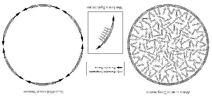
If the self-stressing is higher in a Tensegrity system, its load-bearing capacity is higher too. Using the analogy of the balloon, if a balloon is more inflated, the tension forces in the skin are greater and it is harder to deform it.
The degree of tension of the pre-stressed components is propor tional to the amount of space that they occupy.
As the components in compression are discontinuous, they only work locally. The compression is located in speci fic and short lines of ac tion, so they are not subject to high buckling loads. Due to this discontinuity in compression, they don’t su ffer torque at all.
Tensegrity is the minimal structure that can support a weight and oppose horizontal forces, that uses compression and tension, but experiences no torque.
The systems exhibit the property of synergy where the behavior of the whole systems is not predicted by the behavior of any of their components taken separately.
The resilience ( flexibility) or stiffness of the structure depends on the materials employed, and by their method of assembly. They can be very flexible or very rigid and quite strong. Due to this characteristic, they are very sensitive to vibrations under dynamic loads.
They have the ability of respond as a whole, so local stresses are transmitted uniformly and absorbed throughout the structure.
The response to the loads is non linear. Structures are more flexible under light loads, but their stiffness increases rapidly as the load is higher, like a suspension bridge.
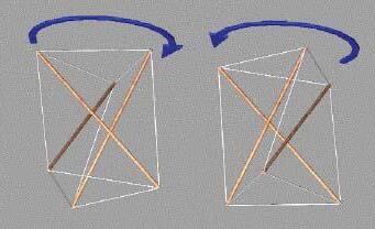
Some Tensegrities, under axial load, experience a rotation around this axe. The direction of this rotation depends on the handedness of the system (enantiomorphic characteristic).
References: Darrell williamson, robert e. Skelton, and jeongheon han, tensegrity structures and their application to architecture chapter 4. Definitions and basic principles equilibrium condi tions of a tensegrity structure
37
FIG 2.11. Diagram explaining enantiomorphic property of prismatic dihedral symmetric structures.
ADVANTAGES
ADVANTAGES OF TENSEGRITY
The mul tidirectional tension network encloses fortuitous stresses where they take place, so there are no points of local weakness.
Due to the ability to respond as a whole, it is possible to use materials in a very economical way, offering a maximum amount of strength for a given amount of building material.
The systems do not experience any kind of torque or torsion, and buckling is very rare due to the short length of their components in compression.
One of the primary advantages of Tensegrity is the deployability and being able to be assembled in short time spans
Modularity is another prime characteristic of the system that makes the system potential of having complex system organization and hierarchies.
The fact that these structures vibrate readily means that they are transferring loads very rapidly, so the loads cannot become local. This is very useful in of absorption of shocks and seismic vibrations.
The spatial defini tion of individual Tensegrity modules, which are stable
by themselves, permits an exceptional capacity to create systems by joining them together. This conception implies the option of the endless extension of the assembled piece.
For large Tensegrity constructions, the process would be relatively easy to carry out, since the structure is self-scaffolding.
Burkhardt sustains that the construc tion of towers, bridges, domes, etc. employing Tensegrity principles will make them highly resilient and, at the same time, very economical.
The kinematic indeterminacy of Tensegrities is sometimes an advantage. In foldable systems, only a small quantity of energy is needed to change their configuration because the shape changes with the equilibrium of the structure.
The response to the loads is non linear. Structures are more flexible under light loads, but their stiffness increases rapidly as the load is higher, like a suspension bridge.
Some Tensegrities, under axial load, experience a rotation around this axe. The direction of this rotation depends on the handedness of the system (enantiomorphic characteristic).
38
FIG 2.12. Highly stable tensegrity structure that can be deployed and reconstructed in very less amount of time.
DISADVANTAGES OF TENSEGRITY
According to Hanaor Tensegrity arrangements need to solve the problem of bar congestion. As some designs become larger, the struts start running into each other.
The same author stated, after experimental research, “relatively high deflections and low material efficiency, as compared with conventional, geometrically rigid structures”
The fabrication complexity is also a barrier for developing the floating compression structures. Spherical and domical structures are complex, which can lead to problems in produc tion.
The inadequate design tools have been a limitation until now. There was a lack of design and analysis techniques for these structures.
In order to support cri tical loads, the pre-stress forces should be high enough, which could be di fficult in larger-size construc tions.
References: Darrell williamson, robert e. Skelton, and jeongheon han, tensegrity structures and their application to architecture chapter 4. Definitions and basic principles equilibrium condi tions of a tensegrity structure
DISADVANTAGES
39
FIG 2.13. Kenneth Snelson’s Sculpture in a process of being installed spanning the water body.
CLASSIFICATION
CLASSIFICATION
CONNECTION BASED
MORPHOLOGY BASED
TENSEGRITY GEODESIC ASSEMBLIES OF MODULES
SINGLE MORPHOLOGY
REGULAR IRREGULAR REGULAR IRREGULAR
CLASS 1CLASS 2
CLASS 1CLASS 2 MORPHOLOGIESMORPHOLOGIESASSEMBLIESASSEMBLIES
X SHAPETENSEGRITY POLYHEDRA PRISMATIC REGULAR TENSEGRITY CELLS
TENSEGRITY CIRCUITS DOUBLE X TRIPLE X TENSEGRITY CLOUD TENSEGRITY TOWERS TENSEGRITY RINGS
The primary aim of classifying the Tensegrity structures on various factors was to study the domain of the system, understand the proper ties and potentials of each classi fied typology based on available research and eventually narrow down the research process for selected typologies that essentially have greater design development potential.
CONNECTION BASED:
A. Tensegrity
B. Geodesic
MORPHOLOGY BASED:
A. Single Morphologies
B. Assemblies
A. SINGLE MORPHOLOGIES
The next level of classi fication of these single modules is based on the parametric properties of the components and the connec tion pattern resulting in Regular and Irregular morphologies.
1. Regular Morphologies
These regular structures can be further classified based on number of struts connecting at each node. A Tensegrity structure is classi fied as a structure of class ‘k’ when I has k number of struts connec ting at each node.
FIG 2.14. Diagram showing the classification of Tensegrity Structures. Refer Appendix for detailed classification listed.
i. Class 1 : These Tensegrity structures essentially have only one strut connecting at each node and at least 3 cables.
a. X-shape:
b. Prismatic Regular Tensegrity Cells:
c. Tensy-Polyhedra
ii. Class 2 : These Tensegrity structures essentially have 2 struts connecting at each node and at least 4 cables.
a. Tensegrity circuits
2. Irregular Morphologies
B. ASSEMBLIES
1. Regular Assemblies
i. Class 1
a. Double-x , Triple-x:
b. Tensegrity towers:
c. Tensegrity cloud:
ii. Class 2
a. Tensegrity rings
2. Irregular Assemblies
40
THEORIES AND METHODS
ANALYTICAL METHODS
KINEMATIC METHOD
STATICAL METHOD
STRUT LENGTH IS CONSTANT AND CABLE LENGTH IS DECREASED CABLE LENGTH IS CONSTANT AND STRUT LENGTH IS INCREASED
STRUTLENGTHISCONSTANTANDCABLELENGTH
TOPOLOGYANDFORCESINMEMBERSISGIVEN
TOPOLOGY AND FORCES IN MEMBERS IS GIVEN OR KNOWN
EQUILIBRIUM STATE IS CALCULATED AND FOUND OUT
ANALYTICALNON LINEAR DYNAMICANALYTICALFORCE DENSITY ENERGY REDUCED
SOLUTIONPROGRAMMINGRELAXATIONSOLUTIONMETHODMETHODCO ORDINATES
CONNELLY AND TERRELL PELLEGRINO MOTRO AND BELKACEM KENNER LINKWITZ AND SCHEK CONNELLY SULTAN
FIG 2.15. Diagram showing the classification of methods used to study Tensegrity Structures. Refer Appendix for detailed classification listed.
CONTEMPORARY RESEARCH AND THEORIES
Although Tensegrity structures have been around for 50 years, it is only recently that they have been analyzed from an engineering viewpoint with focus on system dynamics and mechanics. Most of the research uses Newtonian and Lagrangian dynamics to analyze Tensegrity structures exploring the form finding relationships (limited to symmetric examples) and force displacement associations. However, latest experimentation uses kinematic constraints to determine equilibrium Tensegrity posi tions using various kinematic methods.
Hanaor, in 1992, was one of the first ones to suggest that a kinematic method would be useful for posi tion finding. However, he stated: “Unfortunately, to the best of the author’s knowledge, no func tional algorithms are available to date using the kinematic method.”
Oppenheim and Williams, in 1997 describe in their ar ticles on Tensegrity prisms, use of kinematics and static matrices for incremental posi tion finding of variable geometry truss Tensegrity structures. They also discussed the force displacement relationships in elastic Tensegrity structures and investigated vibrations in these structures.
Sultan, Corless, and Skelton, in 2001 studied finding the equilibrium
posi tions of Tensegrity structures where prestress is allowed using a virtual work approach. They also published a paper on applica tion of a Tensegrity structure as a flight simulator.
Stern and Duff y investigated the self-deployability property of the system with articles presenting equations governing prisms and ini tial Tensegrity posi tions.
Pellegrino and Calladine analyzed statically and kinematically indeterminate structures with matrices.
CLASSIFICATION OF ANALYTICAL METHODS:
A. Kinematic Method
1. Analy tical Solu tion
2. Non-Linear Programming
3. Dynamic Relaxation
B. Statical Method
1. Analy tical Solu tion
2. Force-Density Method
3. Energy Method
4. Reduced Co-ordinates
41
CASE STUDIES

PHYSICAL METHODS
TENSEGRITY WORKSHOP AT SHEFFIELD UNIVERSITY: KONSTATINOS SAKANTAMIS, DR. LARSEN, E. GUTIERREZ
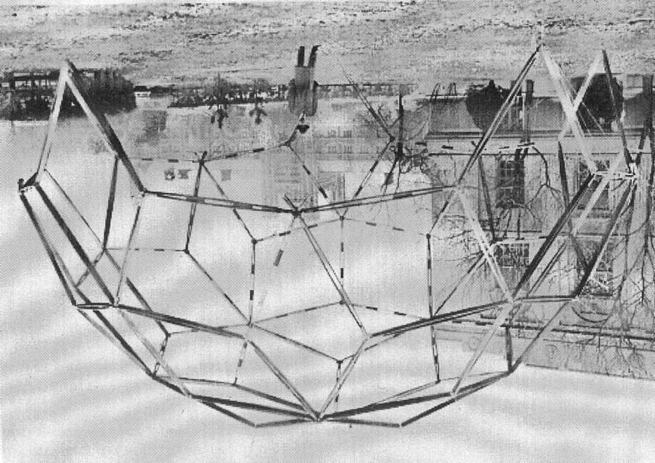
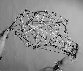
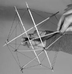
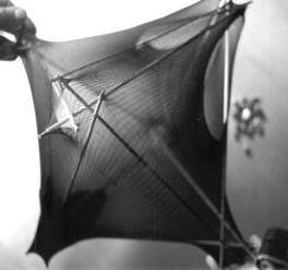
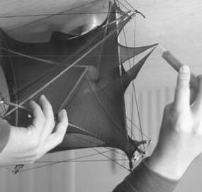
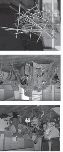
This two part workshop was aimed at developing exclusively only physical methods for form finding and exploring Tensegrity structures. Use of Cocoon methods for experimenting with Tensegri ties that can be developed inside membranes explored immense number of possibilities that Physical experimentation can o ffer using various methods. In addi tion to enhancing the understanding of the system, it also helped in architectural and spatial exploration of the system by designing enclosed spaces. The second part of the workshop further developed on the process and focused on assigning programmatic func tions to these spaces and sculptures thus applying the system to functional designs.
References: JKonstatinos Sakantamis, Dr. Larsen, E. Gutierrez, locomotion of a tensegrity robot via dynamically coupled modules
42
FIG 2.16. Images showing the physical experimentation process to study and design Tensegrity modules combined with cocoon concept.
FIG 2.17. Images showing series of physical models explored at a larger scale to build habitable Tensegrity modules.
ROBOTICS
ADJUSTABLE TENSEGRITY STRUCTURES:
KRISTINA SHEA, BERND DOMER, IAN SMITH
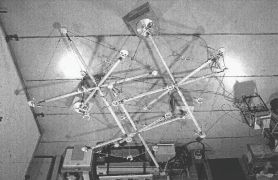
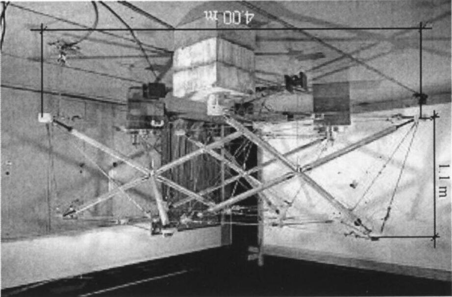
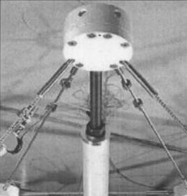
This experiment was aimed at exploring the deployable property of lightweight Tensegrityspace structures for construc ting reusable and modular structures. A full-scale prototype of an adjustable Tensegrity was designed, assembled and tested at Swiss Federal Institute of Technology (EPFL). In their paper, they describe the primary logics of the process. The results show that Tensegri ties behave linearly when subjected to vertical load at single point and non-linearly under several ver tical loads at nodes. The prototype consisted of three modules with each module composed of 4 struts and 24 cables. Telescopic struts are used to modify the geometry and self-stress of the system. 6 degrees of freedom are fixed at 3 supports of this modular geometry that consisted overall 33 joints and 90 elements (struts+cables). By measuring the cable frequency with a laser-based method, tension in individual cables was checked and calculated using
dynamic relaxation method. Numerical modeling was carried to compare physical behavior with analy tical calculations and to be able to predict the behavioral effect of adjusting telescopic struts.
Important highlights and learnings of case study:
- The most important aspect of the design was the joint detaililng, which needed to be pin-jointed, modular and light in order to retain the ease of deployability of Tensegri ties.
- While simulating the geometric non-linear behavior of the Tensegrity structures, it was necessary to consider the nodal fric tion forces.
- Changing the self stress to adapt to changing environments requires Tensegrities to be equipped with sensors and actuators.
References: John rieffel, ryan james stuk, francisco j. Valero-cuevas and hod lipson, locomotion of a tensegrity robot via dynamically coupled modules
43
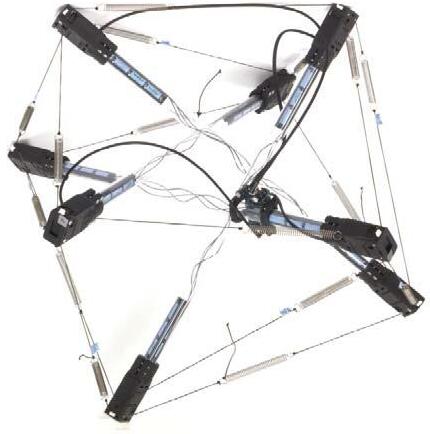
FIG 2.18. Image of the Tensegrity model operated on robotic motors to produce rotational motion at the joints of struts.
FIG 2.19. Image of the rotational joint detail of the strut and cables joinery.
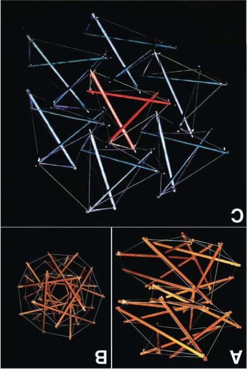
LOCOMOTION OF TENSEGRITY ROBOT:
JOHN RIEFFEL, RYAN STUK, FRANCISCO
VALERO CUEVAS, HOD LIPSON
This investigation exploits the potential of the dynamically stable Tensegrity structures in the field of robo tics due to its relatively high strength-to-weight ratio, resilience to deformation and collapsibility. The modularity of components provide for modular design essen tial in robotics. In the experiment, each module is considered autonomous agent with no explicit inter-modular communication except the tension in the interconnec ting cables, which is the only information transmi tted and received between the modules. Thus the locomo tion arises through the complex inter-play of dynamic forces throughout the structure. Individual modules cable of sensing and a ffecting local tension are designed using servo robot motors capable of continuous rotation and load sensing. These modules are then connected using nylon strings as
time = ~0
time = ~7500 steps
time = ~15 000 steps
tensile elements. Artificial Neural Networks were used for capturing time-sensitive dynamics of the design. An analy tical approach using evolu tionary optimization was used to evolve morphology with the given number of sensors and its locomo tion and gait was successfully simulated and analyzed.
Important highlights of the Experiment:
- The experiment successfully integrates a complex dynamic Tensegrity system with suitable responsive sensory and control system and used the resultant morphological communication for producing locomo tion.
- The experiment also effectively combines the physical tests with digital simulations to produce the mechanical result by using one method to solve the complications of the other.
References: John rieff
44
el, ryan james stuk, francisco j. Valero-cuevas and hod lipson, locomotion of a tensegrity robot via dynamically coupled modules
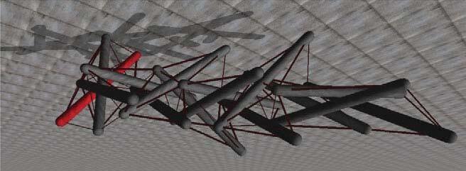
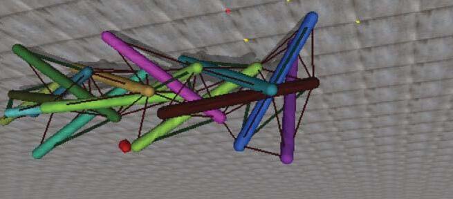
FIG 2.20. Digital image of locomotion simulated by a digital Tensegrity robot.
FIG 2.22. Images showing different time stages of locomotion simulated for Tensegrity robot.
FIG 2.21. Image of the Tensegrity robot used for generating locomotion using Telescopic struts
CONCLUSION
As seen in the case studies and the characteristic properties of Tensegrities, it is fairly tedious and time consuming to explore the vast design space of form-finding using the conventional physical modelmaking methods. It is highly vital to approach this design problem in a more scientific and speci fic process, using algorithmic digital generative form-finding process. This not only enables to explore and test the wide form-finding domain, but also eliminates any biased preferences, thus allowing the result to be generated through purely scientific principles. The process also helps in detailed analysis and investigation of system behavior leading to conclusions and observations that would help in further devising processes to directly generate the desired result.
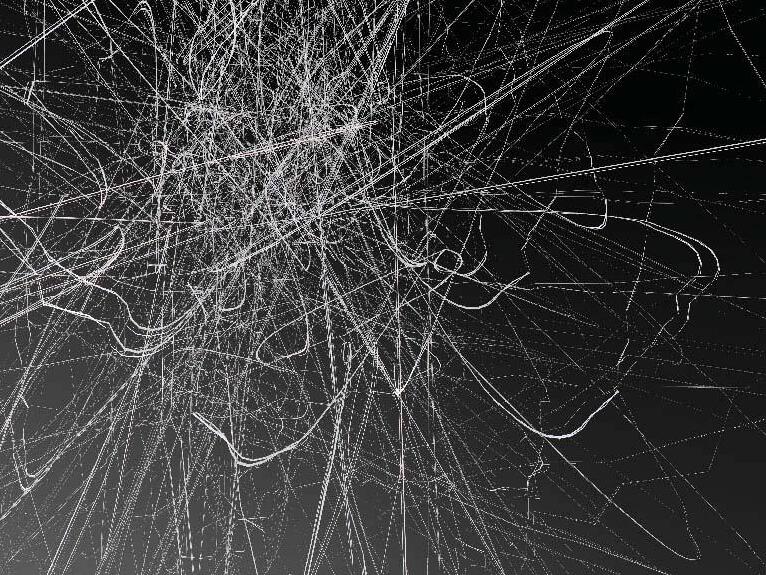
References: FIG 2.23 http://vi.sualize.us/view/7ff4037a987cac6d2b28a47ab4889870/
45
FIG 2.23. Digitally generated image representing complex behaviors
46
EXPERIMENTS
01 PRELIMINARY EXPLORATION Parameters
Regular Tensegrity
Irregular Tensegrity
Critical Analysis
02 GENERATIVE ALGORITHM
Pseudocode
Morphology Generation Evaluation Stage 1
Evaluation Stage 2
03 STRUCTURAL TESTS
Linear Static Analysis
Linear Buckling Analysis
47 CHAPTER 03.
PARAMETERS
GOVERNING PARAMETERS
NOMENCLATURE Example
STRUT LENGTH DIMENSIONS
CABLE LENGTH
CONNECTION
LOGIC NUMBER OF FORM CABLES
NUMBEROFFORM FINDING
NUMBEROFNONFORM NUMBER OF NON FORM FINDING CABLES
NODE FIXED IN X,Y,Z PLANE
DEGREES OF
FREEDOM NODE FIXED IN Y,Z PLANE
NODEFIXEDINZPLANE NODE FIXED IN Z PLANE
PARAMETERS
In order to understand and predict the Tensegrity system behavior, it was necessary to first study the parameters that govern the stable morphology of geometry. The preliminary set of experiments intended to study the effect of variation of these governing parameters on the form and stability of Tensegrity geometries. This experiment was carried out by varying component proper ties in unstable basic seed geometry and consequently observing the resultant variation effect in the stabilized morphology of the geometry.
NOMENCLATURE
GOVERNING PARAMETERS
The primary governing parameters of the stable form of the geometry are the component properties. The lengths of the compressive struts and tensile cables have a defini tive role in the resultant stable morphology. A slight variation in the lengths of either struts or cables resulted in considerable variation in the resultant stable morphology. This property was very signi fi cant in exploring the dynamism of Tensegrity modules in the further research.
The cables were divided further into 2 categories based on their role in form-finding of stable geometries from unstable seeds. The cables that
In order to document the variation of parameters, it was essential to develop a nomenclature that identified each geometry based on its set parameters. This would further help in comparison study of the various relaxed geometries from the same parent basic seed.
48
8H BS 8,10 NODE (7 8 9) ( ) NUMBER LETTER NUMBER NUMBER , NUMBER NUMBER NUMBER BS NODE NUMBER OF STRUTS BASIC SEED ID BASIC SEED NUMBER OF FORM NUMBER OF NON NODE FIXED IN NODE FIXED IN NODE FIXED IN FINDING CABLES FORM FINDING CABLES X,Y,Z PLANEY,Z PLANEZ PLANE
FIG 3.1. Diagram explaining the set of parameters that govern the stability of a Tensegrity structure.
FIG 3.2. Diagram explaining the nomenclature method adopted to represent the digitally explored modules.
MAXIMUM VOLUME
connected the nodes vertically (connec ting top plane nodes with bo ttom plane nodes; shown in blue) were the form-finding cables and were given elastic properties during relaxation process. The cables that connected nodes in the same plane (connected either top nodes only or bo ttom nodes only; shown in black) were the non-form finding cables and were given non-elastic (truss like) properties during relaxation. The struts (shown in red) also were given non- elastic (truss-like) proper ties while relaxing the unstable seed. The number of elastic and non-elastic cables at each node also played a crucial role in the stabilized morphology. Thus the connection logic of the basic seed is an important stability governing parameter.
The non-linear dynamic behavior of the system was further depicted when the variation in degrees of freedom was experimented with. In order to achieve a stable geometry from the basic seed at-least 6 degrees
MINIMUM VOLUME
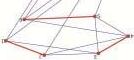
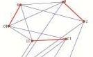
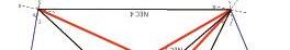
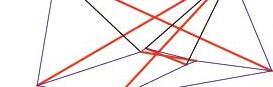
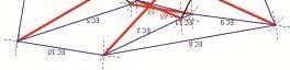
FIG 3.3. An example here shows an unstable 6 strut basic seed with 8 form-finding and 10 non-form-finding cables which was relaxed with 3 different set of nodes namely; node set -7,8,9; node set – 8,10,12 and node set – 7,10,12. Further, 3 orders of same sets were tried out where each node was fixed in different translational axes and relaxed. It was observed that mostly varied morphologies were generated with certain combination producing maximum volume and some combination resulting in flattened minimized volumetric geometries. However, sometimes different combinations resulted in similar relaxed morphologies. Further experimented also showed that certain combinations failed in producing any stable forms.
of freedom among 3 nodes needed to be fixed. Hence a set of 3 nodes was randomly chosen and each of the three nodes was fixed in x-y-z planes, y-z planes, and z plane respec ti vely. Thus 6 degrees of translati onal mo tion were fixed while rotational movement was allowed. This firstly helped in fi xing the geometry in space for relaxation and secondly depicted the multiple stability property of Tensegri ties. Even changing the order of node fixation within same set of fixed nodes resulted in highly varied relaxed geometries.
49 BASIC SEED RELAXATION
SET 8, 10, 12 NODE SET 7, 10, 12
SET 7 ,8
NODE
NODE
,9
SIMILAR MORPHOLOGIES
REGULAR MORPHOLOGIES
REGULAR MORPHOLOGY VARIATION
STRUT NUMBER
DIHEDRAL PRISMATIC TENSEGRITY RADIUS
STRUTNUMBER HEIGHT


TENSEGRITY RINGS
STRUT NUMBER RADIUS
HEIGHT
TRUNCATED
STRUT NUMBER POLYHEDRA RADIUS
HEIGHT
REGULAR MORPHOLOGIES
The next step of investigation involved testing both regular and irregular morphologies under the same set up of experiment for a comparative analysis. The symmetric characteristic feature of regular morphologies implied that any variation in the connec tion logic and nodal degrees of freedom would not result in any variation as the result was essentially the same. Hence the only varying parameter was the component dimension. As the geometry had to be essentially regular, the dimensions of all the component sets had to be propor tionately varied. The digital experimentation was carried by parametrically changing these component properties in Grasshopper interface in Rhinocerous and spatial variation was physically explored using respec ti ve models of each type of regular Tensegrity explored.
The dihedral prismatic regular Tensegrities were varied in strut numbers, planar radius (which essentially was variation in lengths of non-form finding cables), and variation in height (which was variation in lengths of form-finding cables). The same set of parametric experimentation was carried out for other selected Regular Tensegrities namely; Tensegrity rings and Truncated Polyhedral Tensegri ties which has been detailed out in the Appendix sec tion.
A considerable alteration in the enclosed volume was observed in each resultant varied geometry. However, the spatial condi tions and di fferentiation was almost non-existent as all the geometries has consistently similar morphology.
50
FIG 3.4. Diagram explaining the set of parameters that govern the stability of a Tensegrity structure.
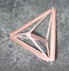
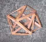
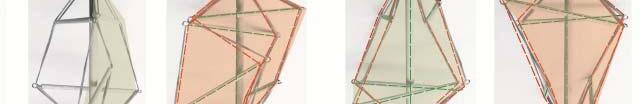
FIG 3.5. Images of physical models of the regular morphologies explored for the spatial conditions exhibited.
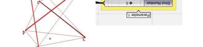
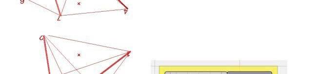
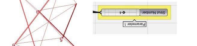
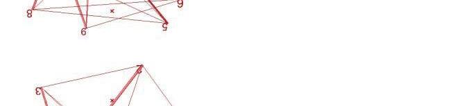
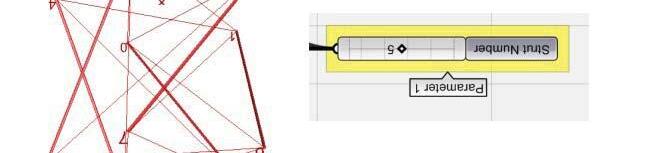
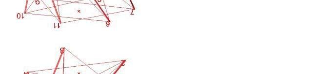
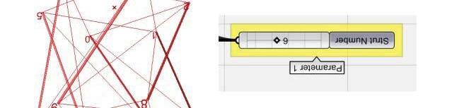
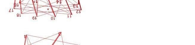
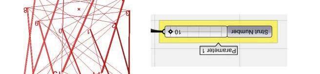
FIG 3.5. Diagram of the Grasshopper parametric digital model or regular tensegrity structure explaining the changing strut number and its corresponding resultant morphology change.
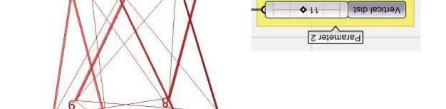
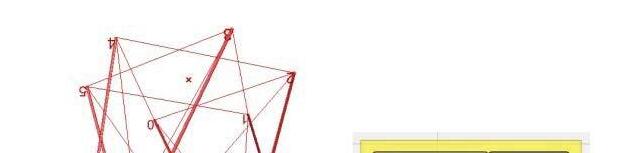
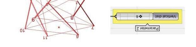

FIG 3.6. Diagram of the Grasshopper parametric digital model or regular tensegrity structure explaining the changing morphology height and its corresponding resultant morphology change.
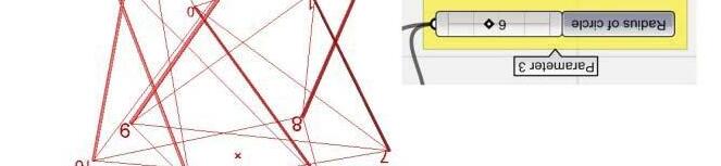


FIG 3.7. Diagram of the Grasshopper parametric digital model or regular tensegrity structure explaining the changing morphology diameter/radius and its corresponding resultant morphology change.
51 STRUT NUMBER HEIGHT RADIUS
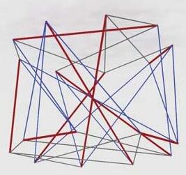
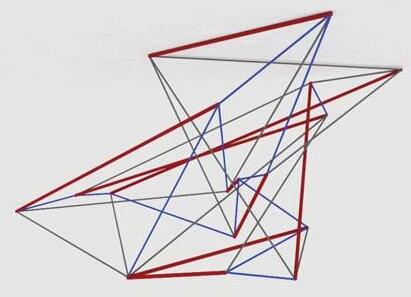
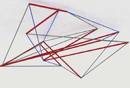
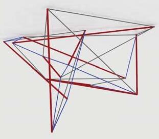
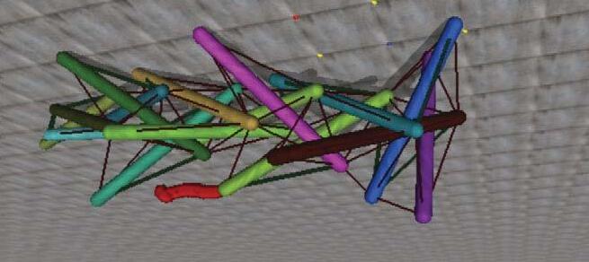
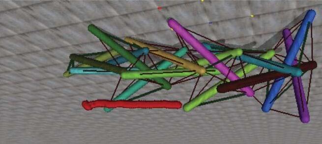
IRREGULAR MORPHOLOGIES
BASIC SEED
RELAXED FORMS
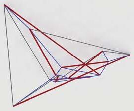
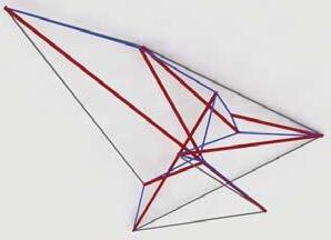
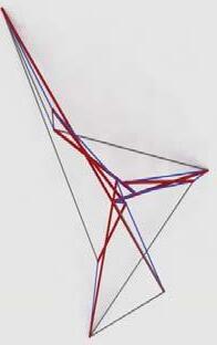
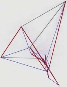
IRREGULAR MORPHOLOGIES
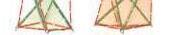
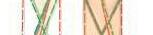
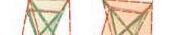
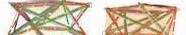
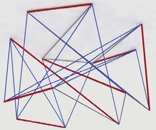
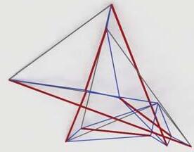
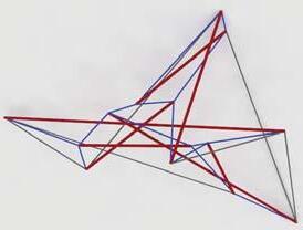
The similar experimentation set up was tested on Irregular morphologies by varying strut number from 4 strut to 9 strut. Subsequently, variation in component dimensions i.e. strut and cable length was tested for resultant variation followed by variation in nodal connec tion logic and degrees of freedom. The diagrams above show examples of the resultant variation; a detailed analy tical study of which is listed in the Appendix sec tion for detailed reference. The variation was limited to one parameter at a time and was carried out in Rhinoceros, while Rhino-membrane plug-in was used for relaxation process.
52
FIG 3.9. Images of physical models of the irregular morphologies explored for the spatial conditions and multiple stable states exhibited.
FIG 3.9. Digitally produced stable states of tensegrity geometry from the single basic seed shown above.
COMPARATIVE ANALYSIS
A comparative analysis between the Regular and Irregular morphologies resulted from the preliminary experiment conclusions was carried out. It was observed that regular morphologies generated proportional variation in the volumes and orientation of resultant geometries. The regular geometries were also more predictable and behaved linearly as opposed to non-linear behavior of irregular Tensegri ties. However, architecturally, irregularly generated morphologies could be di fferentiated in terms of spaces in contrast to the uniform spatial condi tions of regular Tensegri ties. Also, the potential of creating limitlessly varied morphologies of the system provide for possibility of diverse design applications in various topological contexts. This characteristic diversity in irregularly generated modules provides potential of higher complexity and further variation when organized in di fferent hierarchical manner.
CRITICAL ANALYSIS


53
PSEUDOCODE
FIXED PARAMETERS
CLASS CLASS 1 STRUCTURES ONLY 1 STRUT AND 3 CABLES AT EACH NODE
MOVEMENT 3 FIXED BASE POINTS
O1S3CS
VARIATION
DIGITAL APPARATUS
NUMBER OF STRUTS
NUMBER OF SEEDS
6 DEGREES OF FREEDOM FIXED TRANSLATIONAL VECTORS FIXED, ROTATION (, FREEDOM ALLOWED)
MIN = 3 STRUTS
MAX = 9 STRUTS
MIN = 5 VARIED BASIC SEEDS
MAX = 10VARIED BASIC SEEDS
MIN = 3 NODE COMBINATIONS
NODAL SEQUENCE PERMUTATION
MAX = 5
MIN = 3 VARIATIONS
MAX = 6 VARIATIONS
The next step involved setting up the digital apparatus for the experimental exploration of irregular morphologies. Since the design domain was so wide and limitless, it was essential to fix the above listed parameters to limit the boundaries of experiment that involved first generating a widely variant set of unstable basic seeds which would be later relaxed in its mul tiple stable states respectively followed by intensive evaluative elimination process. In order to generate randomly variant ini tial population, a generative script was written in Rhinoscript following the pseudo-code shown alongside. The detailed algorithmic pseudo-code followed is described in the Appendix sec tion for further reference.
STEP 1
The first step involved generation of the unstable basic seed based on the input parameter of number of struts. Considering N number of strut is input in the script, the process generates 2N number of symmetric nodes divided in 2 plane (each plane with N nodes) in a circular equidistant manner. These nodes are then randomly connected by 4N number of links such that each node has 4 set of links. These links are then randomly assigned component proper ties with the limitation of each node bearing one strut and 3 cables. The struts and cables are now randomly exchanged and shu ffled without changing the limitation of number of struts and cables at each node but producing a variant basic seed morphology.
54
FIG 3.10. Diagram explaining the set of fixed parameters and constraints decide for the digital form-finding experiment.
STEP 1
BASICSEED GENERATION
STEP 2
RELAXATION FOR STABLE FORM
STEP 3
PROPERTY OF RELAXED FORM
INPUT = NUMBER RIGID PROPERTY INTERSECTIONS OF STRUTS (N)
STRUTS ASSIGNEED CALCULATE STRUT
CABLES ASSIGNED PRESTRESS VALUES NODES GENERATION

ATLEAST 3 VOLUME OF BOUNDING NODES FIXED BOX OF FORM

ATLEAST 6 DEGREES OF FREEDOM FIXED CONNECTING LINKS
ASSIGNING SSGG PROPERTY

GEOMETRY RELAXED (i RhiMb ) (using RhinoMembrane
BASE AREA OFFORM RELAXED FORM OF FORM

MAXIMUM CLEAR RANDOM SHUFFLING HEIGHT OF GEOMETRY
BASIC SEED
STEP 2
The second step involved obtaining relaxed morphologies from the unstable basic seeds by firstly assigning non-elastic properties to struts and non-form finding cables, and assigning elastic properties to formfinding cables. As mentioned before, the form-finding cables were the links connec ting nodes vertically and non-form-finding cables connected the nodes horizontally in same plane. This was followed by selecting randomly set of 3 nodes and fixing these nodes in x-y-z planes, y-z planes and z plane respec tively, thus fixing 6 degrees of freedom in translational motion. The basic seed was then relaxed using Rhino-membrane plug-in interface.

3.11. Brief Psuedo-code of the process followed in the digital generative algorithmic form-
STEP 3
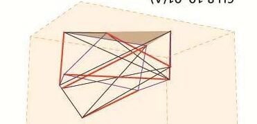
In order to further compare and evaluate the produced geometries, each of the resultant morphologies were digitally tested for their characteristic spatial properties of enclosed volume, base area and clear height. An algorithmic script was wri tten to calculate these properties to be able to calculate the closest proper ties as precise calculation was not only tedious but computationally time-consuming. For volume calculation, bounding boxes enclosing the geometry were generated where each bounding box was aligned with each one of the outer plane of the geometry. The minimum volume of these bounding box was chosen as the geometry volume. Same concept was used to algorithmically calculate base area (by selecting maximum of the various 3-point planar areas) and clear height (by choosing minimum of the various internal single point to 3 point planar distance).
55
FIG
finding of irregular Tensegrity.
BASIC SEEDS
5 STRUTS UNSTABLE BASIC SEEDS
6 STRUTS UNSTABLE BASIC SEEDS
BASIC SEED GENERATION
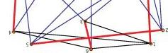
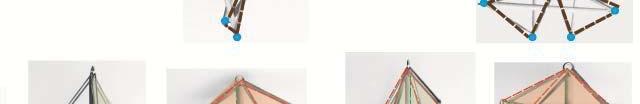
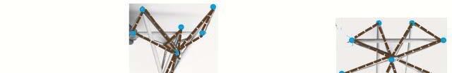
Using the generative script, 40 unstable basic seeds were created with 5 struts, 6 struts, 7 struts, 8 struts and 9 struts geometries. Each basic geometry had an unique connec tion logic and thus would produce high variation in respec tive relaxed modules. It was observed that 6 and 8 struts geometries had a tendency to relax into similar relaxed geometries and produce less variation while odd numbered strut geometries like 5, 7 and 9 struts produced more variant relaxed geometries. Also the number of form-finding and non form-finding cables played a crucial role in stability of geometries. It was observed that geometries with higher ratio of number of form-finding cables and number of ver tical struts produced lesser number of stable geometries.
56
5A BS4,11(i) 1 2 3 4 5 6 7 8 9 10 5B BS6,9(i) 1 2 3 4 5 6 7 8 9 10 5C BS8,7 (i) 1 2 3 4 5 6 7 8 9 10 0 5D BS8,7(ii) 1 2 3 4 5 6 7 8 9 10 0 5E BS6,9(ii) 1 2 3 4 5 6 7 8 9 10
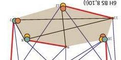
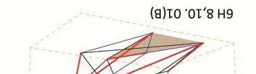
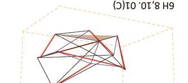
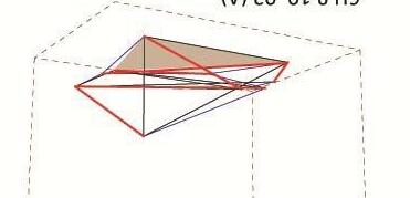
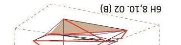
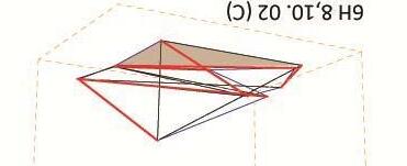
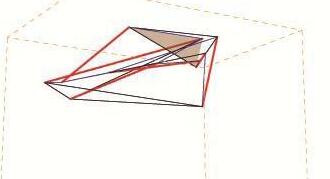
6B BS 10,8(ii) 1 2 3 4 5 6 7 8 9 10 11 12 ii) 1 2 0 6A BS 10,8(i) 1 2 3 4 5 6 7 8 9 10 11 12 0 1 6C BS 6,12.(i) 1 2 3 4 5 6 7 8 9 10 11 12 0 1 1 6D BS 6,12 (iv) 1 2 3 4 5 6 7 8 9 10 11 12 i)7 1 1 2 6E BS 6,12 (ii) 1 2 3 4 5 6 7 8 9 10 11 12 0 1 2 6F BS 6,12 (v) 1 2 3 4 5 6 7 8 9 10 11 12 0 1 1 6G BS 6,12(iii) 1 2 3 4 5 6 7 8 9 10 11 12 1 6H BS 8,10(i) 1 2 3 4 5 6 7 8 9 10 11 12 0 1 1 6I BS 8,10(ii) 1 2 3 4 5 6 7 8 9 10 11 12 1 2 1 2 3 4 5 6 7 8 9 10 11 12 6J BS 8,10(iii)
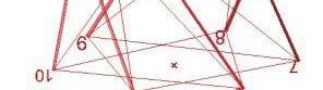
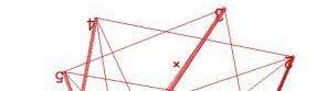
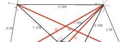
FIG 3.12. Diagram showing the set of all basic seeds randomly produced based on strut numbers.
7 STRUTS UNSTABLE BASIC SEEDS
9
8 STRUTS UNSTABLE BASIC SEEDS
UNSTABLE BASIC SEEDS
57 9A BS 14,13(i) 1 2 3 4 5 6 7 8 9 10 11 12 13 14 15 16 17 18 0 1 8 5 6 9B BS 12,15(i) 1 2 3 4 5 6 7 8 9 10 11 12 13 14 15 16 17 18 0 1 8 9C BS 16,11(i) 1 2 3 4 5 6 7 8 9 10 11 12 13 14 15 16 17 18 1 6 7 8 9D BS 12,15(ii) 1 2 3 4 5 6 7 8 9 10 11 12 13 14 15 16 17 18 0 1 1 6 7 8 1 2 3 4 5 6 7 8 9 10 11 12 13 14 15 16 17 18 9G BS14,13(iii) 1 3 4 5 6 1 9H BS12,15(iv) 1 2 3 4 5 6 7 8 9 10 11 12 13 14 15 16 17 18 3 14 5 6 7 9J BS14,13(iv) 1 2 3 4 5 6 7 8 9 10 11 12 13 14 15 16 17 18 1 3 4 5 1 1 9F BS14,13(ii) 1 2 3 4 5 6 7 8 9 10 11 12 13 14 15 16 17 18 1 1 1 5 6 7 1 9E BS 12,15(iii) 1 2 3 4 5 6 7 8 9 10 11 1213 14 171615 18 1 0 1 1 8 9I BS12,15(v) 1 2 3 4 5 6 7 8 9 10 11 12 13 14 15 16 17 18 0 1 1 1 1 1 1 8
STRUTS
8A BS12,12(i) 1 2 3 4 5 6 7 8 9 10 11 12 13 14 15 16 ) 0 1 1 1 8B BS8,16(i) 1 2 3 4 5 6 7 8 9 10 11 12 13 14 15 16 0 1 2 1 1 6 8C BS10,14(i) 1 2 3 4 5 6 7 8 9 10 11 12 13 14 15 16 1 0 1 1 6 1 2 3 4 5 6 7 8 9 10 11 12 13 14 15 16 8D BS12,12(ii) 1 3 1 5 6 1 2 3 4 5 6 7 8 9 10 11 12 13 14 15 16 8E BS6,18(i) 0 1 1 5 6 7A BS 6,15(i) 1 2 3 4 5 6 7 8 9 10 11 12 13 14 (i) 0 1 1 1 7B BS 6,15(ii) 1 2 3 4 5 6 7 8 9 10 11 12 13 14 15(ii) ) 1 2 ii)3 i) 7C BS 8,13(i) 1 2 3 4 5 6 7 8 9 10 11 12 13 14 0 1 7D BS 10,11(i) 1 2 3 4 5 6 7 8 9 10 11 12 13 14 4 7E BS 10,11(ii) 1 2 3 4 5 6 7 8 9 10 11 12 13 14 ) 1 4 2 7F BS 6,15(iii) 1 2 3 4 5 6 7 8 9 10 11 12 13 14 1 1 7G BS 6,15(iv) 1 2 3 4 5 6 7 8 9 10 11 12 13 14 1 2 4 7H BS 8,13(ii) 1 2 3 4 5 6 7 8 9 10 11 12 13 14 0 1 1 7I BS 6,15(v) 1 2 3 4 5 6 7 8 9 10 11 12 13 14 1 7J BS 10,11(iii) 1 2 3 5 6 7 8 9 10 11 12 13 14 11(iii) 0 1 2 1
RELAXED GEOMETRIES
RELAXATION
The 40 basic seeds produced were relaxed to generate 242 stable forms using the previously mentioned combinations and parameters. The relaxation was carried in RhinoMembrane interface by assigning elastic properties to form finding cables, and non elastic rigid properties to struts and non-form finding cables after fixing at least 3 nodes in 6 translational vectors. There examples of 3 di fferent seeds are shown where each seed produces varied number of stable relaxed forms based on the geometry and connections. There are certain seeds which failed to produce any stable morphologies as shown alongside.
58
5B S6,9(i) .02(A) 5B S6,9 (i). 01(A) 5B BS6,9(i) 1 2 3 4 5 6 7 8 9 10
FIG 3.13. A five strut Tensegrity basic seed and its respective stable relaxed morphologies.
8C BS10,14(i)
FIG 3.14. A eight strut Tensegrity basic seed and its respective 11 stable relaxed morphologies and 4 unstable conditions.
8C S10,14(i).01(A)
8C S10,14(i).02(A)
8C S10,14(i).03(A)
8C S10,14(i).04(A)
8C S10,14(i).05(A)
7H BS 8,13(ii)
8C S10,14(i).01(B)
8C S10,14(i).02(B)
8C S10,14(i).03(B)
8C S10,14(i).04(B)
FIG 3.15. A seven strut Tensegrity basic seed which failed to produce any stable morphologies specifically due to its high number of elastic cables and less vertical struts.
8C S10,14(i).01(C)
8C S10,14(i).02(C)
8C S10,14(i).04(C)
59
1
4 5 6 7 8
1
2 3
9 10 11 12 13 14 15 16 1
1 2 3 4 5 6 7 8 9 10 11 12 13 14
EVALUATION STAGE 1
8C S10,14(i).01(A)
8C S10,14(i).02(A)
8C S10,14(i).03(A)
8C S10,14(i).01(B)
8C S10,14(i).02(B)
8C S10,14(i).01(C)
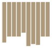
8C S10,14(i).02(C)
VOLUMETRIC EVALUATION
The first stage of evaluation was aimed at eliminating architecturally unusable geometries that enclosed very less volumes or had less clear heights. Hence each of the geometries was evaluated for the enclose volume, base area and clear height. Each of the respec tive data was graphically plo tted as sown in the example above in order to have a comparative analysis and elimination procedure. The geometries with maximum enclosed volume, larger base area and higher clear heights were selected thus eliminating the flatter, condensed and contracted unusable geometries. The evaluation of 242 relaxed modules resulted in selection of 18 usable geometries shown alongside which were further evaluated in next stage.
8C S10,14(i).04(A) 8C S10,14(i).03(B)
8C S10,14(i).05(A)
8C S10,14(i).04(B)
8C S10,14(i).04(C)
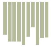

60
1 2 3 4 5 6 7 8 9 10 11 12 13 14 15 16 1 1
8C BS10,14(i)
8C.02(A) 8C.01(A) 8C.02(C) 8C.01(C) 8C.03(A) 8C.02(B) 8C.01(B) 8C.03(B) 8C.04(C) 8C.04(A) 8C.04(B) 8C.05(A) HEIGHT 8C.02(A) 8C.01(A) 8C.02(C) 8C.01(C) 8C.03(A) 8C.02(B) 8C.01(B) 8C.03(B) 8C.04(C) 8C.04(A) 8C.04(B) AREA 8C.05(A) 8C.02(A) 8C.01(A) 8C.02(C) 8C.01(C) 8C.03(A) 8C.02(B) 8C.01(B) 8C.03(B) 8C.04(C) 8C.04(A) 8C.04(B) VOLUME
8C.05(A)
FIG 3.16. A eight strut Tensegrity basic seed and its respective stable relaxed morphologies long with the evaluative comparative graphs of volumes, base areas and heights of each of the relaxed geometries.
FIG 3.17. The set of 19 chosen morphologies after the first evaluation stage.
S6,9(i) .02(A)
61
5B
6F
6A
6G
6H
7E
7E
7F
7I
8A
8A
8C
9B
12,15(i).
9B
12,15(i). 01(B) 9B S 12,15(i). 03(A) 9I S12,15(v).01(A)
5A S4,11(i). 01(A)
6,12 (v).01 (B)
10,8. 01(A)6D 6,12 (iv). 03(A)
6,12(iii). 03 (A)
8,10. 01(A) 7C S 8,13(i).03 (A)
S 10,11(ii). 02(A)
S 10,11(ii). 01(A)
S 6,15(iii). 03(C)
S 6,15(v). 01(A)
S12,12(i).02(C)
S12,12(i).02(B)
S10,14(i).01(C) 9A S 14,13(i).01(B)
S
02(A)
S
EVALUATION STAGE 2
FABRICATION BASED EVALUATION
The second stage of evaluation intended to access the fabrication ease of the modules. The first step involved eliminating geometries with intersecting struts as it was structurally not feasible to fabricate. The above shown evaluation of 3 out the 18 modules has the 3rd example with intersecting struts and thus the geometry gets eliminated followed by evaluation for uniformity in component dimensions for fabrication ease. In order to access this regularity in lengths of struts and cables, values for each strut and cable length is plo tted graphically. A flatter line graph implied higher uniformity in component dimensions. The graphs alongside show relative strut and cables lengths for each of the 18 geometries, which were ranked based on fitness criteria (uniform components). This procedure helped in retaining economically buildable modules and eliminated geometries with too many varying strut and cable
lengths. The 6 filtered out modules shown alongside were then selected for further structural tests and analysis. A detailed documenta tion of the second stage of evaluation is listed n the Appendix sec tion for reference.
62
0 1000 2000 3000 4000 5000 6000 7000 S:5S:1S:6S:2S:3S:4 0 1000 2000 3000 4000 5000 6000 7000 STRUT LENGTH STRUT LENGTH CABLE LENGTH S3 S4 S1 S6 S2 EC 3 EC 7 EC 2 EC 6 EC EC 8 EC 12 EC 11 EC 9 EC 1 NEC 5 NEC 6 NEC 2 NEC 4 NEC 1 NEC 3 X X X Z Z Y Y Y STRUT LENGTH STRUT LENGTH CABLE LENGTH NEC 4 NEC 2 NEC 3 S2 S3 S5 S4 S1 EC 6 EC 9 EC 8 EC 10 EC 2 EC 5 EC 7 EC 11 NEC 1 0 1000 2000 3000 4000 5000 6000 7000 EC:4 EC:3 EC:11 EC:9 EC:2 EC:10 NEC:3 EC:1 EC:7 EC:5 EC:6 EC:8 NEC:1 NEC:2 NEC:4 0 1000 2000 3000 4000 5000 6000 7000 S: 5 S: 1 S 3 S 2 S 4 0 1000 2000 3000 4000 5000 6000 S:5S:4S:1S:2S:3 7000 0 1000 2000 3000 4000 5000 6000 7000 EC:6 EC:5 EC:7 EC:4 EC:3 EC:2 EC:1 NEC:1 NEC:6 NEC:4 NEC:5 NEC:8 NEC:3 NEC:7 NEC:2 STRUT LENGTH STRUT LENGTH CABLE LENGTH S3 S1 S5 S2 S4 EC 2 EC 1 EC 1 EC 7 EC 5 EC 6 NEC 7 NEC 8 NEC 4 NEC 3 NEC NEC 2 NEC 5 X X Y Y Z Z Z X X Y Y Y
FIG 3.18. Examples of 3 of the 19 selected geometries along with the second stage evaluative graphs of strut lengths and cable lengths and intersection points of the struts.
FIG 3.19. Ranking of the selected 19 morphologies based on fitness criteria focussing on fabrication ease.
CABLE LENGTH
FIG 3.21. Selected 6 modules after evaluation stage two.
FIG 3.20. Comparative evaluation graphs of Struts lengths and cable lengths of each individual morphology.
5A S4,11. 01 (A) 5C S8,7 .03 (B) 6A S 10,8(i). 01(A)
6D S 6,12 (iv). 03(A)
6F S 6,12 (v).01 (B) 6G S 6,12(iii). 03 (A) 6H S 8,10. 01(A)
7C S 8,13(i).03 (A)
7E S 10,11(ii). 01(A)
7E S 10,11(ii). 01(B)
7F S 6,15(iii). 03(C
7I S 6,15(v). 01(A)
8A S12,12(i).02(B)
8A S12,12(i).02(C
8C S10,14(i).01(D)
9A S 14,13(i).01(B)
9B S 12,15(i). 02(A)
9B S 12,15(i). 03(A)
9I S12,15(v).01(A)
63 0 1000 2000 3000 4000 5000 6000 7000 123456789 5A
01
5C
6H
8,10. 01(A) 7C
8,13(i).03 (A) 7E
10,11(ii). 01(A) 7E
10,11(ii). 01(B) 7F
6,15(iii). 03(C ) 7I
01(A)
8A
9A
14,13(i).01(B) 9B S 12,15(i). 02(A) 9B S 12,15(i). 03(A) 9I
STRUT LENGTH
AFTER EVALUATION 0 1000 2000 3000 4000 5000 6000 7000 12345678910111213141516171819202122232425262728
S4,11.
(A)
S8,7 .03 (B) 6A S 10,8(i). 01(A) 6D S 6,12 (iv). 03(A) 6F S 6,12 (v).01 (B) 6G S 6,12(iii). 03 (A)
S
S
S
S
S
S 6,15(v).
8A S12,12(i).02(B)
S12,12(i).02(C 8C S10,14(i).01(D)
S
S12,15(v).01(A)
RANKING
5A S4,11(i). 01(A) 5B S6,9(i) .02(A) 6A 10,8. 01(A) 7E S 10,11(ii). 02(A) 7F S 6,15(iii). 03(C) 8C S10,14(i).01(C)
STRUCTURAL ANALYSIS
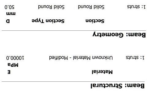
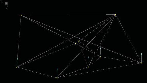
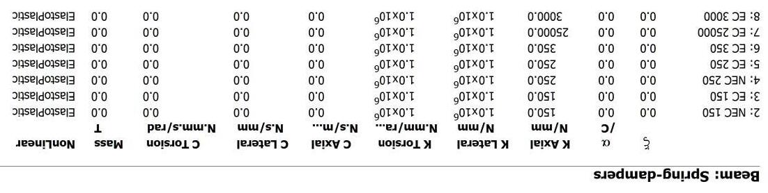
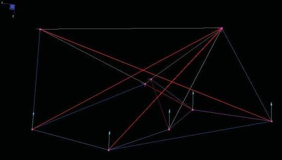
STRAND ANALYSIS
Structural Analysis in Strand was carried out for the selected modules to simulate the deflection of the nodes and the buckling threshold of the struts under the assigned load and to get the appropriate geometry of the components.
For the digital setup, Struts are assigned as beams with elastic modulus of ___________. Cables are defined as springs with axial stiffness of each cable is inversely propor tion to its length according to the relation “Axial Stiffness = (alpha / length of the cable)”.
Based on the geometry, minimum three nodes are fixed on the ground in the translational x, y and z axis keeping the rotational movement free. The other nodes are subjected to a load of 1000 N in the (-z) direc tion.
Each module is tested for three strut cross-sec tion diameter value viz. 20mm, 50mm and 75mm and under three load cases with varying pretension values of 0.02, 0.01 and 0.001 in the tension cables.
64
FIG 3.22. 5 strut module tested in Strand7 for stability using the alongside given values of stress and elasticity.
LINEAR STATIC ANALYSIS
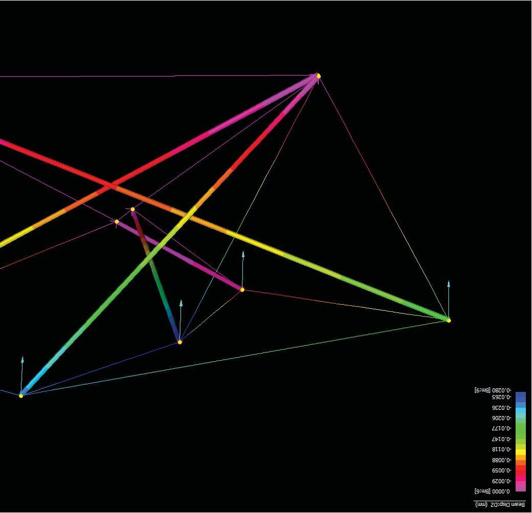
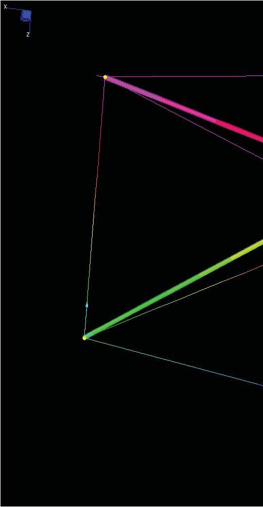
Linear Static Analysis (LSA) and Linear Buckling Analysis (LBA) are carried out for all these 9 di fferent combinations of Strut Diameter and the Pretension in the cables.
LSA is carried out to study the deflection in the geometry caused due to the designed load and LBA estimates the Load at which the struts will begin to buckle and is governed by the strut diameters.
Based on the inferences of the above experiments, the final strut geometry and cable pretension value is decided. In certain cases to get the desired stability for the designed load, combinations of di fferent strut dimensions is explored.
This exercise helped in classifying the geometries based on their structural stability and load bearing capacity.
65
NEC 4 X X Z Z Y Y NEC 2 NEC 3 S2 S3 S5 S4 S1 EC 6 EC 9 EC 8 EC 10 EC 2 EC 5 EC 7 EC 11 NEC 1
FIG 3.23. Linear Static Analysis test of the below shown module in Strand7 interface.
LINEAR BUCKLING ANALYSIS
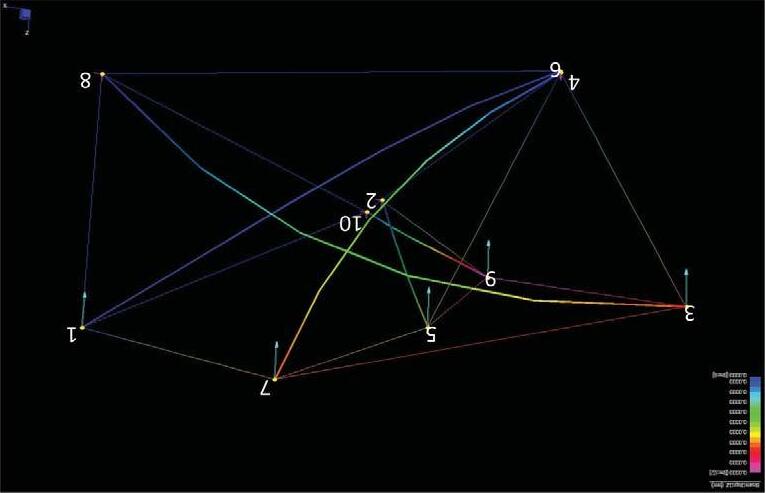
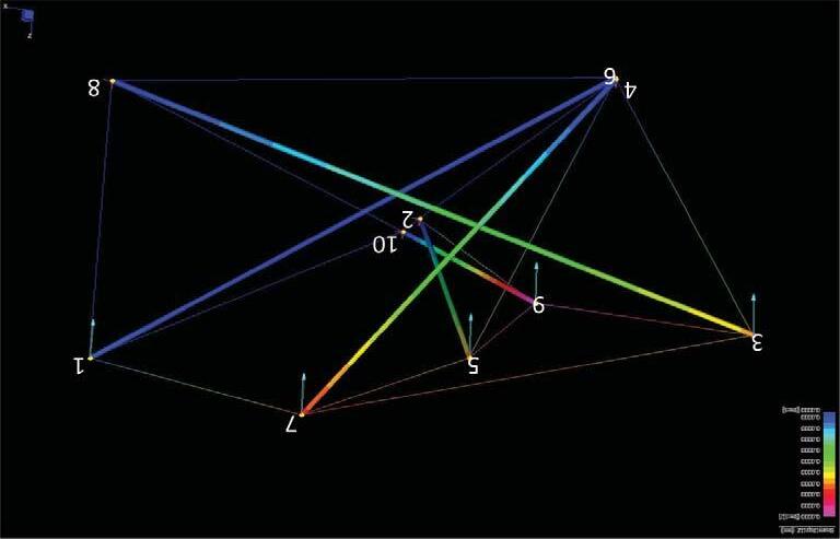
COMPONENT DIMENSIONS
The structural analysis done for one of the 6 six selected module is shown above where the buckling loads for the structure was calculated. Since the buckling load was lower than the required design load the struts had to be redesigned by changing the diameter in order to increase the strength of the structure and to ensure stability under cri tical load of 1000N. The diagrams alongside the same experiment and tests done on the other 5 design modules to redefine the stable dimensions.
66
COMPONENTS Material Modulus (N/ SQ MM) Diameter(MM) LOAD(N) PRETENSION STRUTS Wood 1e + 4 20 1000 0.01 CABLES Steel 2.1e + 8 8 COMPONENTS Material Modulus (N/ SQ MM) Diameter(MM) LOAD(N) PRETENSION STRUTS Wood 1e + 4 50 1000 0.01 CABLES Steel 2.1e + 8 8 NEC 4 X X Z Z Y Y NEC 2 NEC 3 S2 S3 S5 S4 S1 EC 6 EC 9 EC 8 EC 10 EC 2 EC 5 EC 7 EC 11 NEC 1
FIG 3.23. Linear Buckling Analysis test of the alongside shown module in Strand7 interface shows the module buckling under the alongside dimensions.
FIG 3.24. Linear Buckling Analysis test of the alongside shown module in Strand7 interface shows the module stability and no bucklingunder the alongside dimensions.
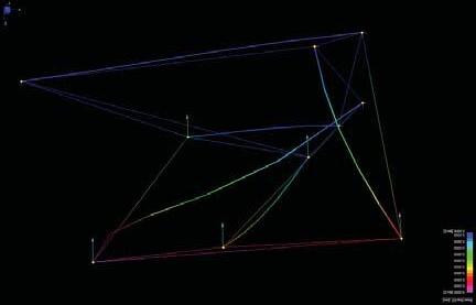
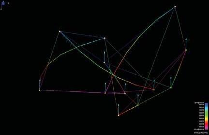
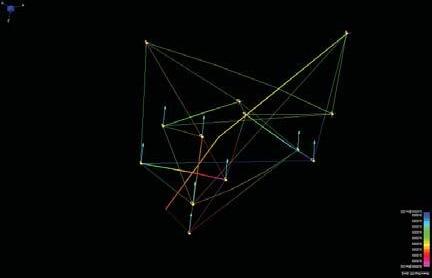
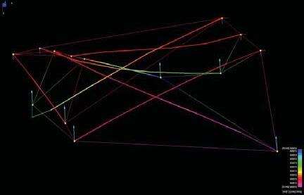
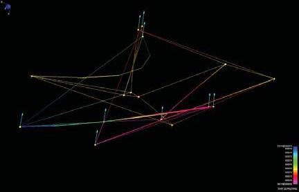
OPTIMIZED RESULT
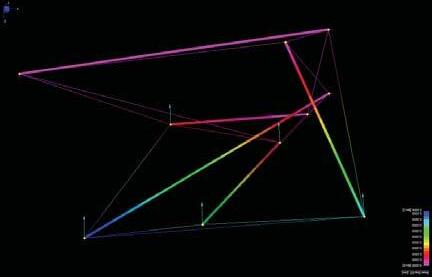
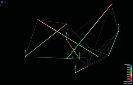
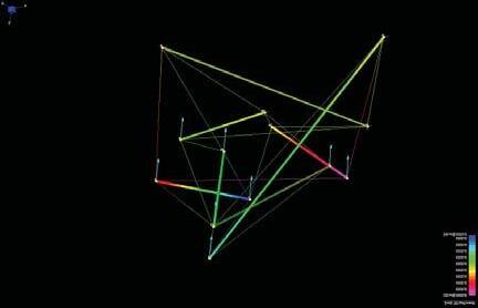
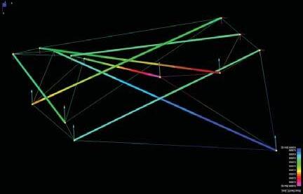
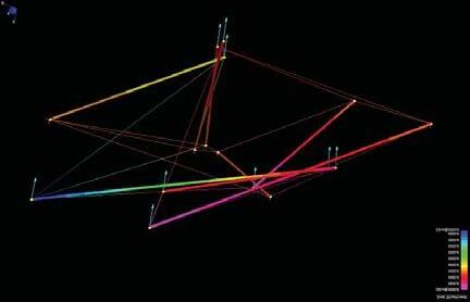
67
S6 S1 S4 S3 S2 S7 S8 S5 EC 2 EC 7 EC 10 EC 3 EC 13 EC 6 EC EC 5 NEC 6 NEC 10 NEC 5 NEC 2 NEC NEC 1 NEC 8 NEC 7 NEC 3 X X X Z Y Y S3 S4 S6 S7 S5 S1 S2 EC 3 EC 15 EC 1 EC 9 EC 12 EC 6 EC 8 EC 5 EC 10 EC EC 11 EC 13 EC 7 NEC NEC NEC 2 NEC NEC 5 X Y Y S2 S2 S7 S4 S3 S1 S6 EC 3 EC 8 EC 7 EC 2 EC 6 EC 4 EC 9 EC 5 EC 11 NEC 6 NEC 2 NEC 10 NEC 5 NEC 1 NEC 7 NEC 3 NEC 4 X Z Y S3 S1 S4 S2 S5 S6 EC 1 EC 8 EC 7 EC 6 EC 4 EC 5 EC 2 EC 3 NEC NEC 9 NEC 8 NEC 4 NEC 5 NEC 1 NEC 10 NEC 7 NEC 6 X X Z Z Z Y Y Y S3 S1 S5 S2 S4 EC 2 EC 1 EC 1 EC 7 EC 5 EC 6 NEC 7 NEC 8 NEC NEC 3 NEC 1 NEC NEC 5 Z Y X
FIG 3.25. Linear Buckling Analysis test of the alongside shown modules in Strand7 interface with their respective buckled and stable geometries.
68
DESIGN DEVELOPMENT
01 SPATIAL EXPLORATION
Catalogue of Orientation Module Selec tion Set
02 MULTIPLICITY
Rotation of Struts
Telescopic Struts
03 MEMBRANES
Spatial Enclosures
Structural Tests
04 MODULE ORGANIZATION
Variant Morphologies
Same Morphologies
69
CHAPTER 04.
MULTI-ORIENTATION STABILITY
One of the most unique proper ties of Tensegrities is the ability to retain its stable form in any posi tion and orientation irrespective of external forces. Furthermore, under external loads, the stability of the module is further increased due to increase in prestress values of the cables that effectively accentuate formal stability. This ability of Tensegrity modules coupled with ability to inherently display di fferentiation in spatial quali ties due to irregularity resulted in generating series of variation of spatial quali ties and architectural condi tions by merely changing the orientation of same module in di fferent ways. In order to explore this spatial variation potential of each of the modules, an exercise of cataloguing di fferent orientation for each of the selected 6 modules was carried out. The cataloguing exercise helped in comparing each orientated module for its di fferentiation of enclosed, semi-enclosed and covered spaces.
CATALOGUE OF SPATIAL DIFFERENTIATION
This propor tion of spatial di fferentiation implied varied structural performance characteristics of being covered space, partition element or cantilevered area. It also played a key role in further selection of modules for design exploration based on design and contextual requirements. A detailed catalogue of di fferent orientations of each of the 6 selected modules is listed in the Appendix for reference.
70
MULTI-FUNCTIONALITY
5A S4,11(i). 01(A)
FIG 4.2. Catalogue of various spatial configurations and orientations of the above selected module.
SPATIAL ORIENTATION CATALOGUE
71
5A
01
1 2 3 5 6 7 8 9 10 1 3 6 7 8 9 10 5A S4,11. 01 (1-8-10) 1 2 3 5 6 7 8 9 10 1 3 5 6 7 8 9 10 12 3 5 6 7 8 9 10 5A S4,11. 01 (2-4-8) 1 2 3 5 6 7 8 9 10 1 2 3 5 6 7 8 9 10 1 2 3 5 6 8 9 10 5A S4,11. 01 (3-5-7) 12 3 5 6 7 8 9 10 5A S4,11. 01 (4-8-10) 1 2 3 5 6 7 8 9 10 1 2 3 5 6 7 8 9 10 1 2 3 5 6 7 8 9 10 1 2 3 5 6 7 8 9 10 4 1 2 3 4 5 6 7 8 9 10 1 2 3 4 5 6 7 8 9 10 PLAN
S4,11.
(1-5-7-8)
5A S4,11. 01 (2-4-8)
5A S4,11. 01 (1-8-10)
SELECTED DESIGN MODULES
Based on the site studies and spatial requirements of the programs and context (which is listed in following chapter), the above 5 design modules were selected from the catalogue for appropriate functions. The next step of the design development was to test these modules for possibility of dynamic spatial re-configuration.
COMPONENT MANIPULATION
As mentioned in the earlier chapter, the dimensions and lengths play a very crucial role in the stable configuration of the relaxed form. This property of producing variant stable forms with slight change in the dimension was used to achieve dynamism in the form by manipulating component lengths and orientation. This experiment was carried out
to test each of the selected design modules for possibility of distinctly usable spatially reconfigured organization. This characteristic feature was the key to achieving program based dynamic performance of the system.
The manipulation of the component proper ties was carried out in 2 methods: (a) by changing the length of the struts or (b) by rotating the struts with one end fi xed at the base and relaxing the structure again in Rhino-membrane after re-assigning component proper ties of elasticity.
The experiment was limited to manipulating only one strut at a time; only the 3 struts with one end fixed at the base were manipulated. The length change was limited to either increasing or decreasing by 1.5 m at the free end of the fixed strut. The rotational change was also limited to a + 100 or - 100 in the x-y plane about the fixed end of the strut. In both the cases the module sometimes produced a large spatial variation and reconfiguration, but most of the times resulted in swaying of the structure as seen in the example alongside.
72
MULTIPLICITY
5C
7E
10,11(ii).
S8,7 .02(A) (6-7-8) 6A S 10,8(i). 01(A) (1-2-3)
S
01(B) (7-9-12)
FIG 4.3. Set of selected design modules from the spatial catalogue based on suitability for chosen programs.
FIG 4.4. Diagram showing the selected stable module orientation and its changed stable states post rotation and telescopic length change of the struts.
ROTATIONAL CHANGE
5A S4,11. 01--- (1-8-10) BS
ROTATION
(1-8-10)--- Strut @ 15A (1-8-10)--- Strut @ 85A (1-8-10)--- Strut @ 10
ROTATION
ROTATIONAL CHANGE
The example above shows a 5 strut module tested for rotational manipulation of component. The change would be achieved by using pin jointed detailing with freedom for rotation at the fixed end. The strut would require to be rotated manually as per the need to re-configure the space. A detailed exploration of spatial re-configurations obtained by strut rotation for each of the 5 selected design modules is listed in the Appendix sec tion for reference
73
+10
1 2 3 4 5 6 7 10 9 8 -10
5A
+10 +1.5M -1.5M -10 +10 +1.5M -1.5M -10 +10 +1.5M -1.5M -10
respective stable states
after rotating one of the 3
a time)
FIG 4.5. Selected module and its
achieved
struts (one at
by 10 degrees in x-y plane.
TELESCOPIC CHANGE
M LENGTH
1.5 M LENGTH
TELESCOPIC CHANGE
The example above shows the same 5 strut module tested for length manipulation of component. The change would be achieved by having telescopic struts that could be increased and decreased by 1.5 m at the free end of each of the 3 fixed struts. The telescopic change would require to be triggered manually as per the programmatic need or user need to reconfigure the structure for enclosed space. However, due to pre-stressed nature of the system, this mechanism would require either use of motors or dismantling of structure and re-assembly of the module.
A detailed digital exploration of the telescopic manipulation of struts for each of the design modules and the respec tive resultant variation is listed in the Appendix sec tion for reference.
74
5A
1 2 3 4 5 6 7 10 9 8 5A
+10 +1.5M -1.5M -10 +10 +1.5M -1.5M -10 +10 +1.5M -1.5M -10 +1.5
S4,11. 01--- (1-8-10) BS
(1-8-10)--- Strut @ 15A (1-8-10)--- Strut @ 85A (1-8-10)--- Strut @ 10
-
FIG 4.6. Selected module and its respective stable states achieved after telescopically changing one of the 3 struts (one at a time) by 1.5 m at the free end.
DESIGN MODULES
FIG 4.7. Selected set of final design modules and its respective stable states achieved after rotating one of the 3 struts (one at a time) by 10 degrees in x-y plane. The selected module set thus contains 3 nondynamic and 2 dynamic modules.
75
5A S4,11. 01--- (1-8-10) BS 1 2 3 4 5 6 7 10 9 8 5A S4,11. 01---(2-4-8) BS 1 3 5 6 7 9 10 2 8 5B S8,7 .03 --- (6-7-8) BS 1 3 4 5 6 7 9 10 2 8 1 3 4 5 6 7 9 12 11 10 2 8 6A S 10,8(i). 01(A)---(1-2-3) BS 7E S 10,11(ii). 01(B) --- (6-9-12) BS 14 3 4 5 6 7 9 12 11 13 10 2 8 -10 ROTATION +10 ROTATION -10 ROTATION
MEMBRANE ENCLOSURE
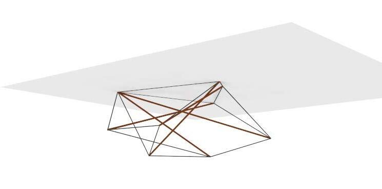
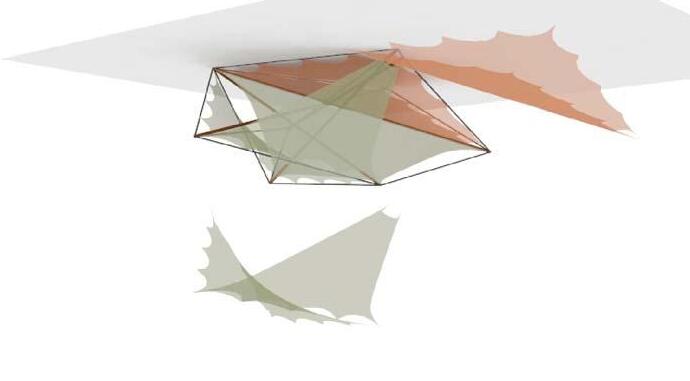
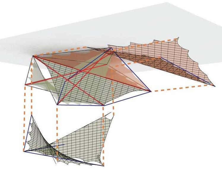
MEMBRANE ENCLOSURE
The next design step was to start creating enclosures in these design modules by not only retaining the spatial di fferentiation of spaces but rather enhancing it. This was done by adding tensile membranes to the structure by fixing the ends to cable ends and fixing the edge completely to the strut length. The membranes were further relaxed to achieve its stable form by using a relaxation script in Rhino-Script. Shown alongside are the membrane enclosures for all the five selected design modules and their respective multiple states.
76
FIG 4.7. Diagram showing addition of enclosing membranes to the structure.
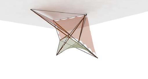
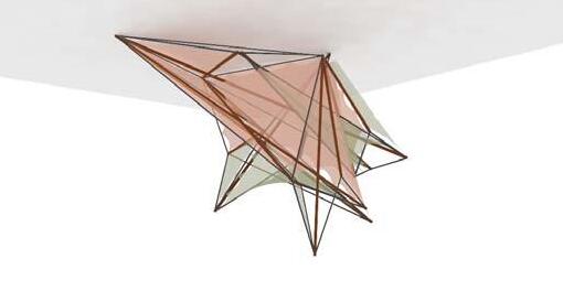
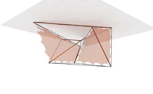
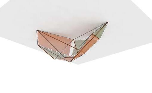
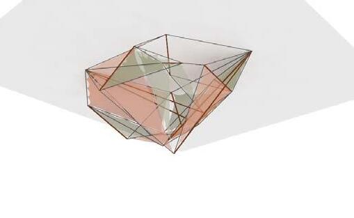
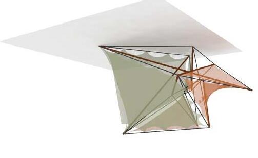
77
5A S4,11. 01 (1-8-10)
5C S8,7 .02(A) (6-7-8)
6A S 10,8(i). 01(A) (1-2-3)
7E S 10,11(ii). 01(B) (7-9-12)
FIG 4.8. Diagram showing addition of enclosing membranes to the structure of the selected modules.
MEMBRANE STRUCTURAL ANALYSIS
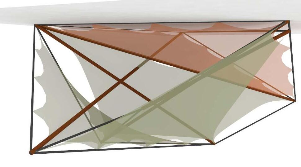
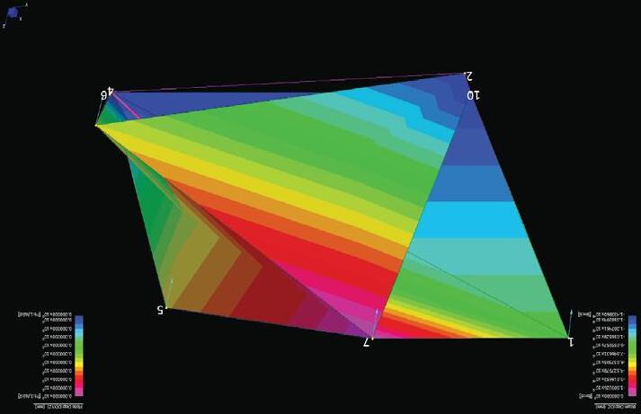
STRAND ANALYSIS
In order to understand the structural implications of the membrane addi tion, the modules were again tested under same condi tions as before for structural stability. It was observed that the tensile membranes affected the buckling loads as the structure had now started failing at lower threshold loads. This implied that the strength of the structure required to be regained by further increasing the strut diameter. The diagram above shows the Linear Buckling Analysis Test carried out on the 5 strut design module when an addi tional membrane layer is added.
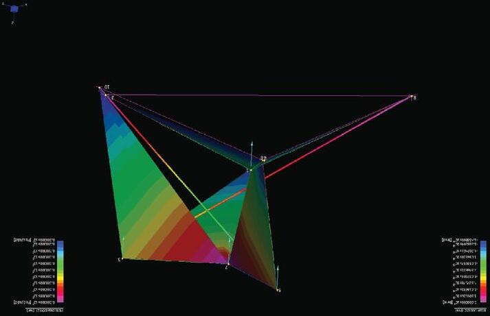
78
FIG 4.9. Diagram showing linear buckling analysis of the alongside shown selected module subjected under the design loads.
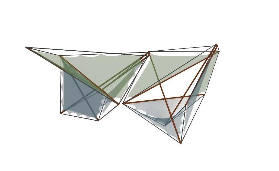
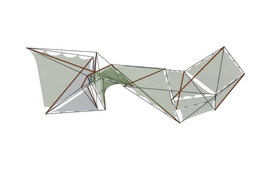
MODULARITY
The ability of Tensegrity structures to exist independently as modules and still have the potential of developing continuity by having hierarchical organization and connec tion logics is highly unique and useful. This capability generates scope of developing and designing inter-modular spaces that would have potential of being architecturally usable. This would also provide for ability to expand usable spaces when larger volumes are needed for certain functions.
ORGANIZATION LOGIC
The diagram above shows 2 examples of di fferent design modules connected for generating architecturally usable spaces. There exists both di fferentiation and continuity of spaces within the organized module. The
MODULE ORGANIZATION
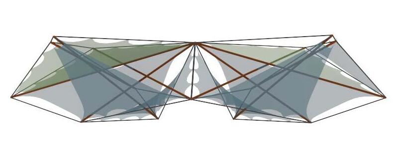
connection logic was to create inter-modular usable spaces which would generate semi-open and semi-enclosed public spaces. These spaces can be designed for community based programs and this organization logic by infiltrating and stitching together the interstitial spaces in urban fabric.
The same process can be experimented for connecting same modules as shown in the example above.
79
FIG 4.10. Diagram showing inter-modular organization and connection strategy for different modules.
FIG 4.11. Diagram showing inter-modular organization and connection strategy for same modules.
80
DESIGN PROPOSAL
01 REVISED DESIGN STRATEGY
02 SITE Mumbai City Urban Context
03 PROGRAM STUDIES
Existing Programmatic Typologies
Activity v/s Time-scale Study
04 ORGANIZATION STRATEGY
Program based Organization Hierarchical Expansion
05 TEST PROPOSAL
Architectural Intervention
Design Application
06 CONSTRUCTION DETAILS
Joints and Connec tions Fabrication Assembly
81
CHAPTER 05.
REVISED DESIGN STRATEGY
DESIGN STRATEGY
RESIDENTIAL +
DYNAMIC WORKSHOP SPACES MODULES RESIDENTIAL + COMMERCIAL SPACES
COMMERCIAL + WORKSHOP SPACES
NON DYNAMIC
RESIDENTIAL EXTENSIONS MODULES INDUSTRIAL SHEDS
DEPLOYABLE TEMPORARY COMMERCIAL SPACES MODULES MARKET SPACES
DESIGN STRATEGY
COMMERCIALSPACES
Based on the learnings and observations of the Design Development stage, the design strategy was revised and adapted to suit the speci fic site requirements and program needs. The idea was to use the existing site program units as guiding points for the placements of the newer design modules. In order to achieve this goal, the site was studied in detail by selecting a small typical cluster for test application. The exi ting programs and ac tivities were studied in terms of their time-scales of use and spatial needs during use. The inferences from this study helped in placing the highly dynamic modules in those par ticular areas that exhibited this need for changing program and space. The other non- dynamic modules were placed in places which exhibited need for the similar spatial orientations for the respective functions.
82
FIG 5.1. Diagram showing revised design approach.
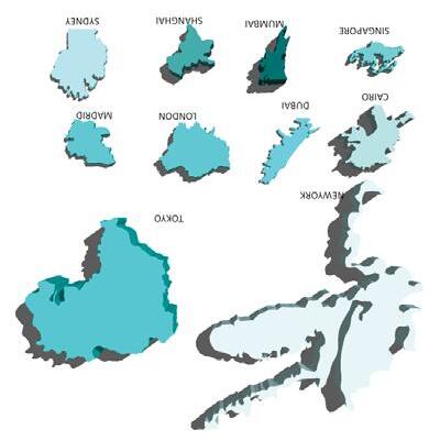
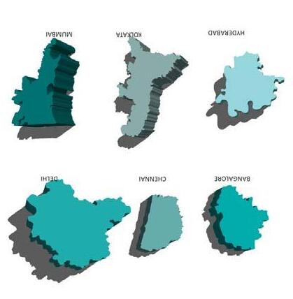
Mumbai is one of the largest developing ci ties and one of the most thriving urban blends of lifestyle and living condi tions. With a population of almost 13.8 million located in an area of 603.4 sq km, Mumbai houses one of the largest service sectors of the country contribu ting to 5% of the country’s GDP. With limited land, yet unlimited growth opportuni ties resulting in perpetual rural to urban migration of as huge as 0.12 million annually, the city of Mumbai faces urban densi ties of as high as 22,922 per sq km. The overly dense living condi tions resul ting due to an acute lack of land for expansion have exaggerated the subsequent urban infrastructure crisis of transport, water supply, sanitation, drainage, electricity and massive under-supply of affordable housing, thus lowering the urban standards of living. Moreover, constant siltation and land reclamation have resulted in ecological problems of rivers being reduced to waste drains and flooding during monsoons.
SITE MUMBAI CITY
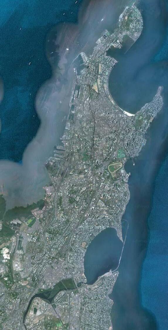
83
MUMBAI CITY
FIG 5.3. Diagram showing population densities of different Indian cities.
FIG 5.4. Satellite image of Mumbai City and its sub-urban regions.
FIG 5.2. Diagram showing population densities of different International cities.
CONTEXT - INFORMAL SETTLEMENTS


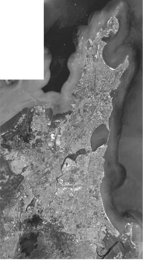
SLUM SETTLEMENTS

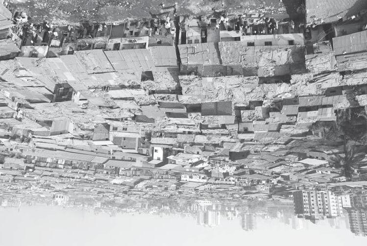
Paradoxically, while more than 50% of the urban populati on lives in the poor housing condi tions of informal slum settlements like Dharavi spread over 8% of the total land; these slums also house one of the biggest industries of produc tion and processing. With residential and work spaces coinciding, these living condi tions reflect extremely dynamic multipleuse of space with respect to the activities, time and the working patterns. There is constant adaptation of the limited available space in order to provide for the changing needs based on the number of users and types of use. There is a very typical migration and settlement pattern observed in the use and expansion of these informal slum settlement areas. As most of the settlement units are illegally constructed structures, there is a constant rapid change in the types of users renting the living spaces. While the types and number of users vary from single fresh migrants working as industrial labor to small and large family units se tting up their home based small scale industrial units; the use of space varies from
small to large scale industrial workshop spaces and residential units. With immense redevelopment pressure, there is a need for designing a mass housing system that reflects the existing complex living patterns and adapts to these rapidly changing social condi tions and contexts at varying time scales. The redevelopment building systems need to reflect properties of adaptability, flexibility, modularity, cost effective and ease of mass produc tion and fabrication. The spatial variation requirements arising from the change in program needs to be achieved through reconfiguring structural organizations from same amount of material. The dynamic reconfiguration process is a func tion of time based changes; spanning from a short time period like daily user based and environmental changes to long term changing user needs involving growth of number of users, or change in use of space.
References:
FIG 5.5. http://blog.propertynice.com/4-firms-drop-out-of-dharavi-plan/
84
Slums and informal settlements of Mumbai
FIG 5.4. Diagram showing satellite image of Mumbai city and areas occupied by illegal slum settlements.
FIG 5.5. Image showing the dense living conditions of the Slum settlement urban areas.
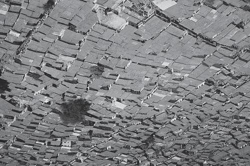
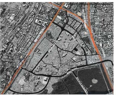
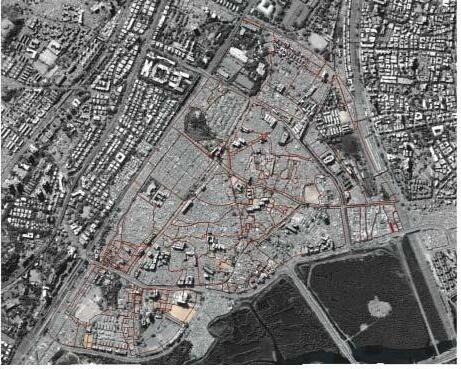
DHARAVI SLUM SETTLEMENT
Dharavi area is widely known for its organically growing dense illegal settlements of slum dwellers. While it mainly serves as living spaces for numerous households, it is simultaneously a huge industrial area housing many produc tion and processing workshops and industries of varied scales. There are several overlapping layers of spatial programs and uses for optimal space management in this overly dense settlement area. The site studies show overlaps of residential and commercial spaces, residential and workshops units, industrial and living spaces, produc tion and commercial units. Thus for a system that serves the varying need of program and space usage, a mixed context like this settlement would be a perfect model for experiment and applying the system.
References:
FIG 5.6. http://blog.propertynice.com/4-firms-drop-out-of-dharavi-plan/
FIG 5.7,8,9. Design Cell Study, Kamla Raheja Vidyanidhi Institute of Architecture
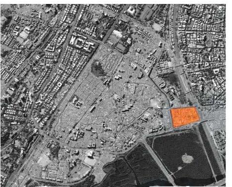
85
FIG 5.6. Image showing the dense living conditions of the Dharavi slum area.
FIG 5.7. Satellite Image showing the boundaries and major road connections surrounding Dharavi slum area.
FIG 5.8. Satellite Image showing the internal road connections of the Dharavi slum area.
FIG 5.9. Satellite Image showing the zoomed in site called 13th Compound area and its location with respect to Dharavi settlement.
PROGRAM TYPES
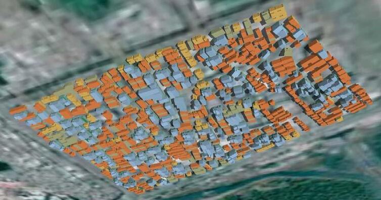
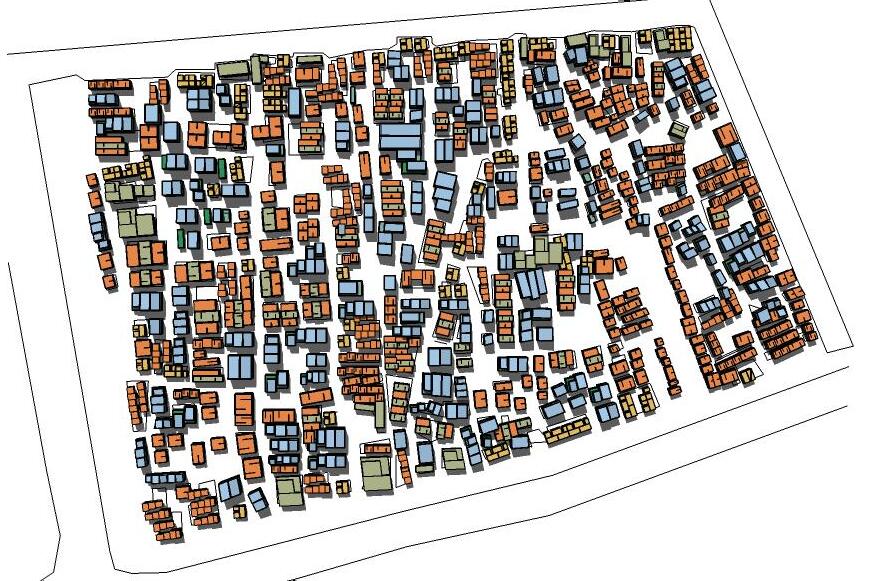
13TH COMPOUND SITE
The site is located at one of the most crucial junc tions of the Dharavi area, with a land-use pattern that exhibits blend of residential, commercial, workshops and industrial units. The primary reason for selec tion of the site was to have a context that reflected user-based and use-based variation of func tional spaces at varied time scales. The location of this site is prime due to its commercial edge, and respec tive industrial and produc tion workshop units. The secondary use of residential units as small scale workshops and produc tion units also essentially demonstrate need for dynamic spaces at varied time scales. Thus the 13th Compound seemed ideal due to its diverse use pattern and the changing need of spaces which is the fundamental concern of the research.
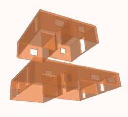
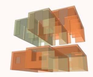
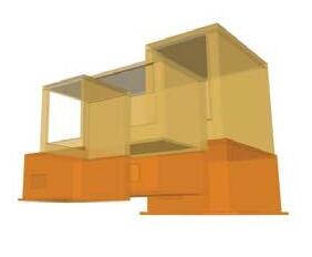
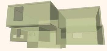
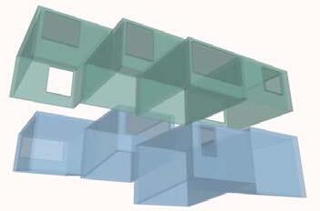
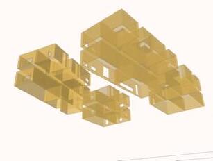
86
RESIDENTIAL UNITS LEGEND RESIDENTIAL + WORKSHOP UNITS RESIDENTIAL + COMMERCIAL UNITS SMALL SCALE WORKSHOP UNITS LARGE SCALE INDUSTRIAL UNITS COMMERCIAL UNITS
FIG 5.9. Image representing the urban fabric and mixed overlapping program units in the site area.
FIG 5.10. Site plan representing the urban fabric and mixed overlapping program units in the site area.
FIG 5.11. Diagrams showing the different program units and the respective typical spatial conditions.
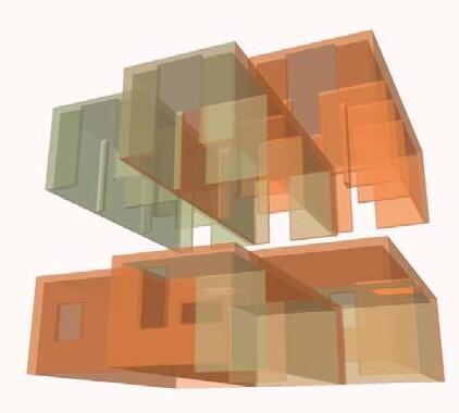
ACTIVITY TIME LINE

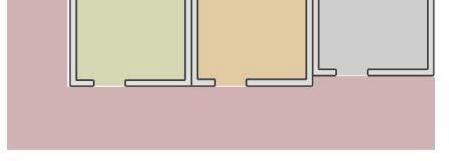
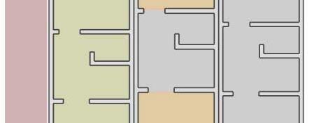
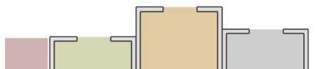
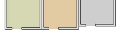
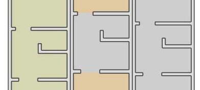
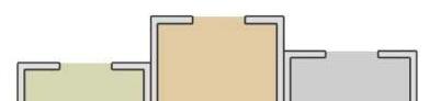
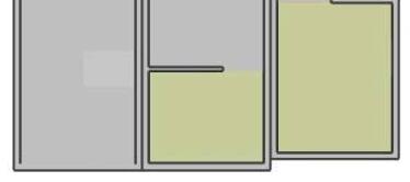
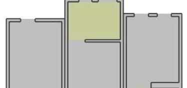
Under the pressures of rapidly changing lifestyles, there is constant adaptation in the living condi tions and daily ac tivity patterns of the residents of the areas. There is a constant overlap of programs within limited spatial boundaries based on the user needs. The space gets used for residential and workshop usage or commercial use at di fferent times of the day and year. These daily cycles reflect the need of changing spaces
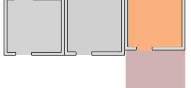
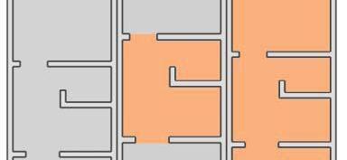
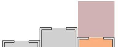
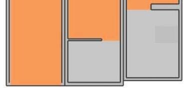
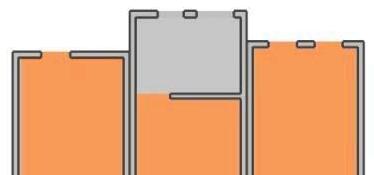
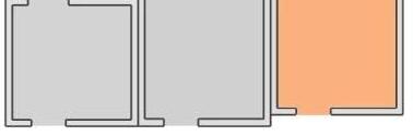
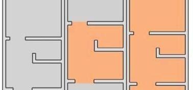
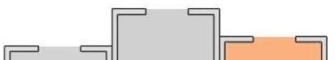
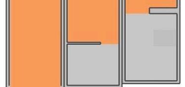
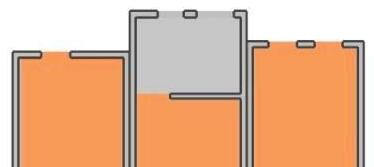
that adapt as per the user needs. The above diagram shows one of the activity mappings of the residential and workshop spaces depic ting the space usage at di fferent times. This study was crucial during the design organization process in order to decided the placement of dynamic modules. A detailed study of the ac tivity mapping of all the di fferent programmatic typologies,at di fferent times is listed in the Appendix section for further reference.
87
8.00 –12.00 12.00 –17.00 R OUT SPACE RESIDENTIAL WORKSH 17.00 –1.00 1.00 –8.00 OP 8.0
SPACE USAGE TIME LINE
FIG 5.12. Diagram showing the study map of activity and respective spatial usage at different times of the day.
ORGANIZATION STRATEGY

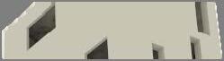
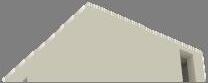
STAGE 1

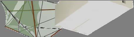
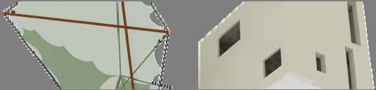
STAGE 2
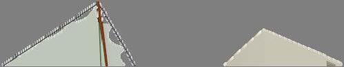
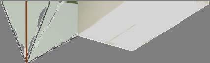
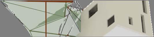
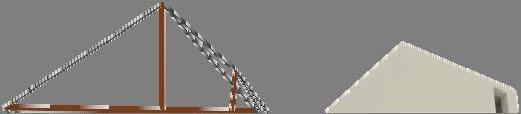
STAGE 3
EXTERIORINTERSTITIAL EXTERIOR INTERSTITIAL SPACES FOR USE
CONFIGURATION OF SPACE WITHINWARD WITH INWARD ORIENTATION (WORKSHOPS)
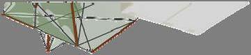
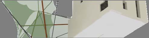
RECONFIGURED SPACE WITH OUTWARD ORIENTATION (COMMERCIAL)
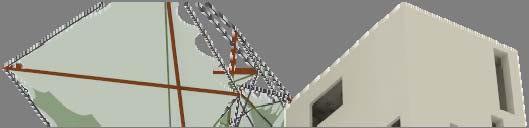

DYNAMICALLY RECONFIGURED EXPANDED SPACES FOR VARYINGUSES VARYING USES
MODULE PLACEMENT
The inferences from the previous acti vity mapping and ti me-scale study helped in deciding the placement of dynamic and non-dynamic modules based on program requirements. Thus the modules started getting organized around the existing blocks in order to enable extra flexible space usage as per the user needs and times. These flexible exterior space could be transformed from being introverted workshop spaces to a more outward orientated commercial space due to the dynamic flexibility of the design modules.
88
FIG 5.13. An example showing the variation resulted in the spatial orientation due to change in the dynamic module condition.
FIG 5.14. Examples of the above shown module and its orientation and placement with respect to existing unit (both the stable states).
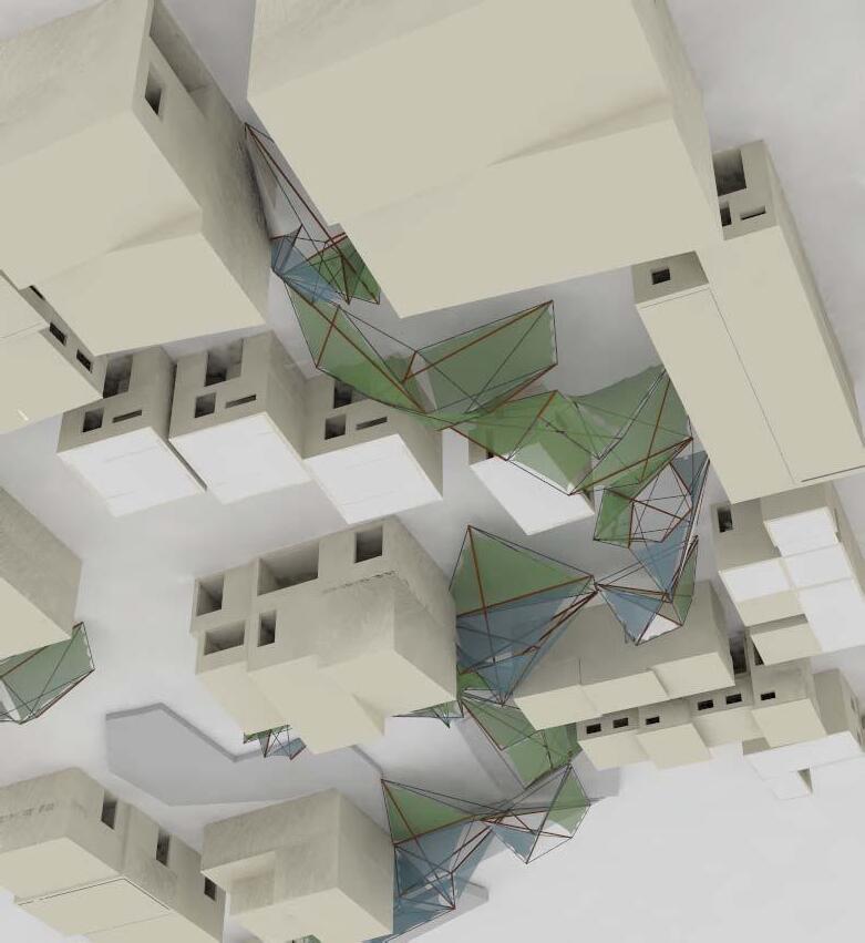
INFILTRATING MODULES
The module organization and connec tion system resulted in the design penetrating the site through its redundant interstitial spaces and using them for temporary extended programs. These organized modules started developing hierarchy based on the penetration extents with te periphery modules being more outwardly orientated, to the central ones being more introverted orientation. This organization and infiltration design strategy also starts generating an order and circulation pattern in the other-wise highly chao tic and unorganized urban fabric.
HIERARCHICAL ORGANIZATION
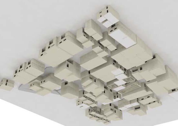
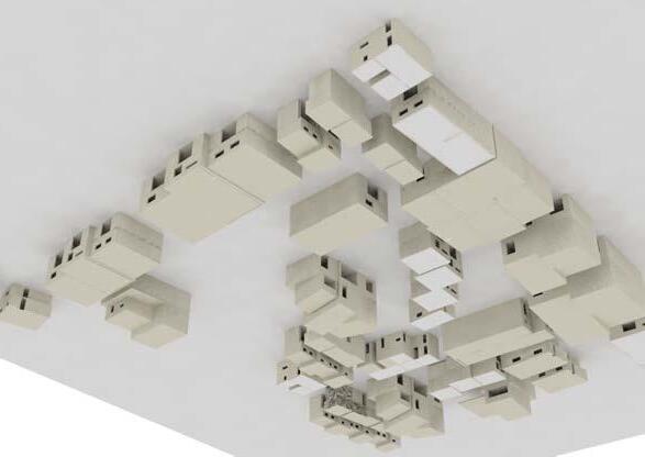
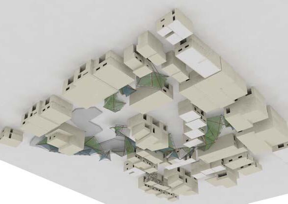
89
FIG 5.15. View showing the modules organized in site cluster.
FIG 5.16. View showing the exiting pattern of units in the site.
FIG 5.17. View showing resultant site conditions after removal of units.
FIG 5.16. View showing the proposed design after replacing the removed units with design modules.
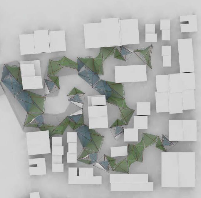
OPEN / CLOSED PROPORTIONS
The proposed design, as can be observed, not only results in re-organizing the chao tic site condi tions, but also enhances the living condi tions of the place by increasing the ratio of the open spaces to built areas as compared to the existing condi tions. This resultant design thus provides a su fficient urban open space, which was much essential in the highly dense overcrowded settlement areas.
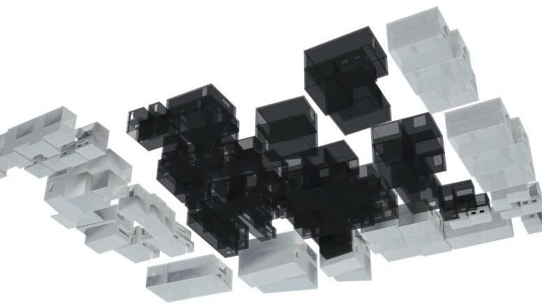
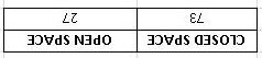
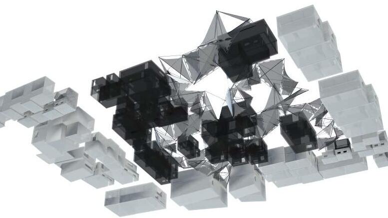
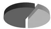
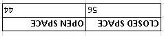
90
PLAN
DESIGN -
FIG 5.18. Site plan of the proposed design with the design modules and organization.
FIG 5.19. Site plan showing the proportion of open and closed spaces on the existing site.
FIG 5.20. Site plan showing the proportion of open and closed spaces on the site after the design.
DESIGN ELEVATIONS
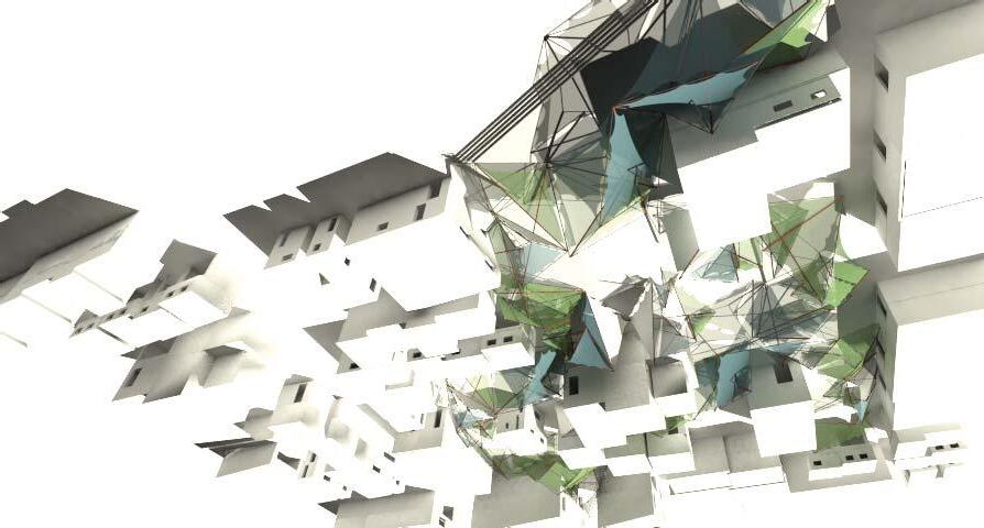
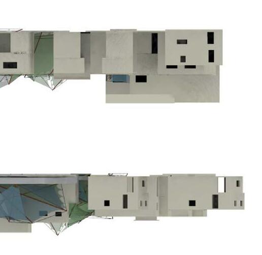
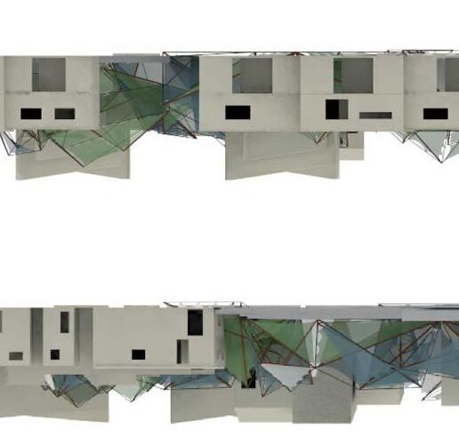
FIG 5.21. View of the proposed design showing the interstitial spaces and community areas infiltrating into the existing urban fabric.
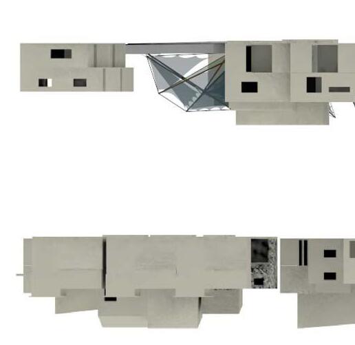
91
FIG 5.22. East Elevation of the site
FIG 5.23. South Elevation of the site
DESIGN - VIEWS
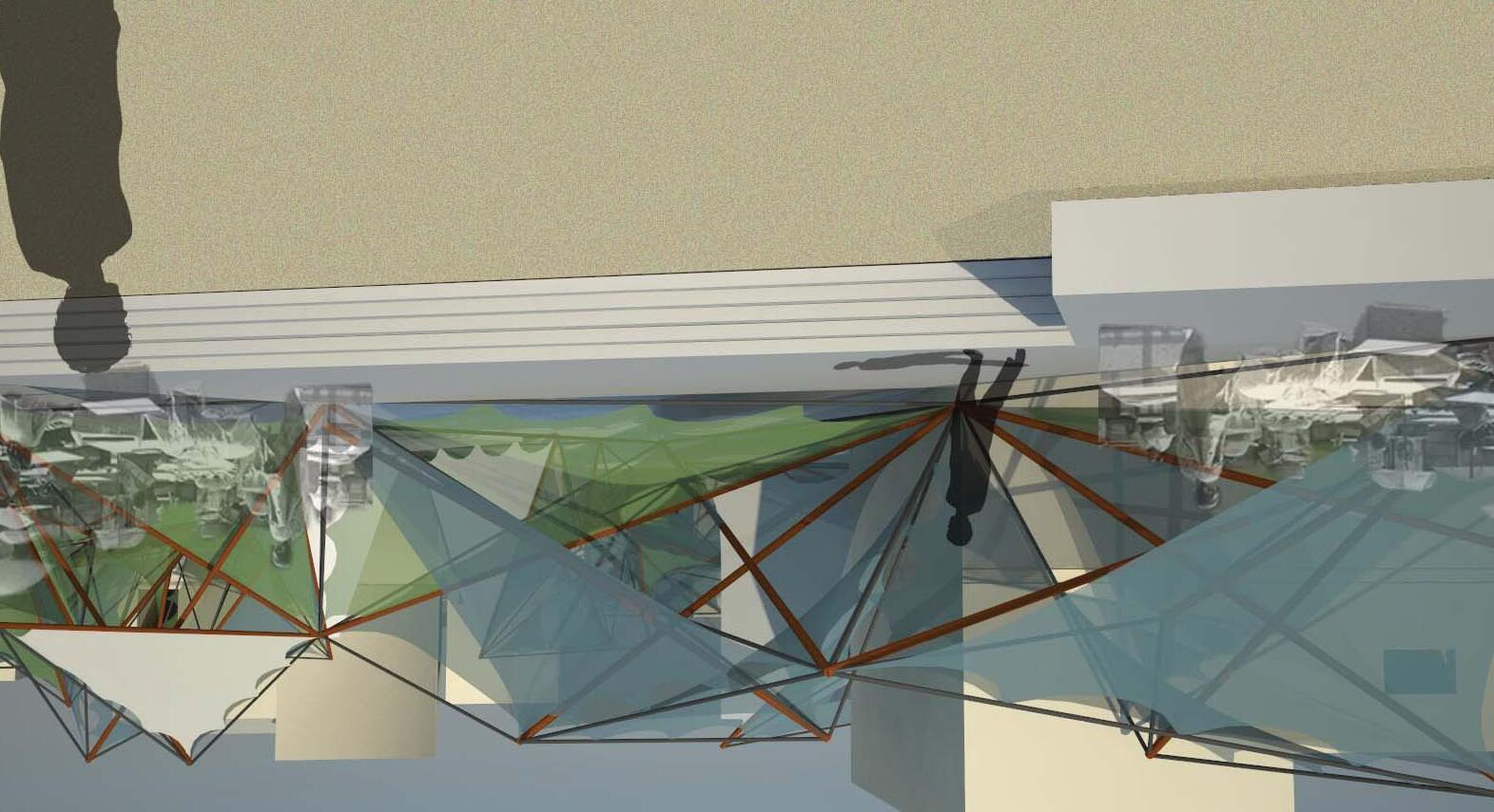
DESIGN APPLICATIONS
As shown in the rendered views, the proposed design is imagined to be used to enhance the social living condi tions and interac tions in the site by being used as market spaces, commercial areas, workshop extensions, industrial sheds, semi-open infrastructures facility spaces (like schools, dy care centres etc). These structures can be dismantled when not in use or reconfigured as per user needs. Thus the urban lifestyles and living patterns get reflected and adapted by the structural system.
92
FIG 5.24. Rendered view of the community market space with semi-open commercial markets and cantilevered stalls.
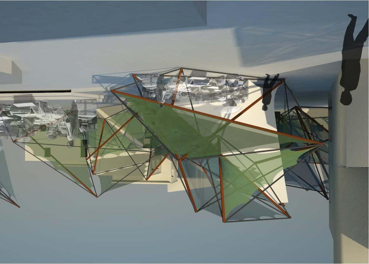

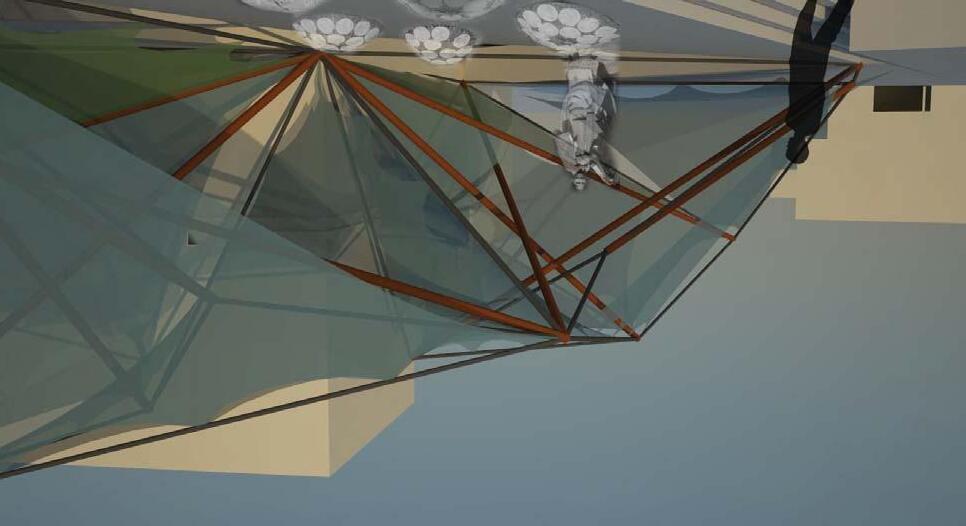
93
FIG 5.25. Rendered view of the exterior workshop spaces extended in the exteriors of the existing housing modules.
FIG 5.26. Rendered view of the semiopen small scale manufacturing units with house-hold scale industries.
COMPONENTS - JOINTS
JOINT CONNECTIONS
INTRINSIC CONNECTIONS
STRUT CABLE
STRUT GROUND
STRUT MEMBRANE
CABLE MEMBRANE
MEMBRANE MEMBRANE
EXTERNAL MODULE GROUND XTRNA CONNECTIONS MODULE MODULE
CONNECTIONS
MODULE SITESTRUCTURE – SITE STRUCTURE
The accuracy and precision in the joints and connec tions of the elements of the modules is the key to the stability and strength of the structure as the system solely relies on the connec tion logics of its components. It is therefore highly essential to study and detail out the joint connec tions for better overview of the required of construc tion methods, techniques and sequence. The above diagram briefly lists down the various types of joints and connec tions that the structure needs.
94
FIG 5.27. Diagram showing list of different types of joints and connection existing in the system.
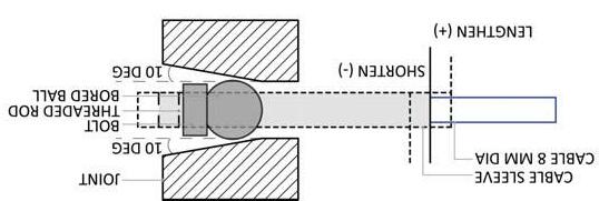
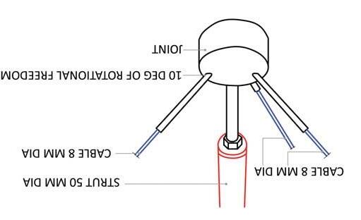
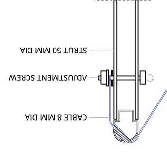
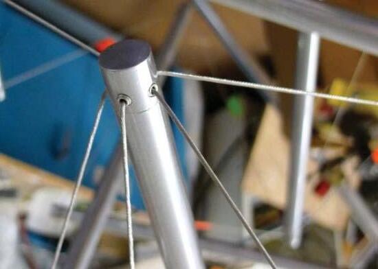
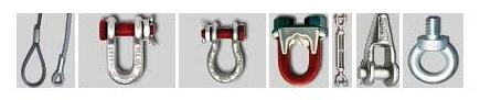
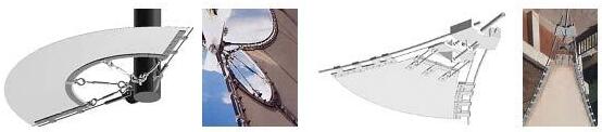
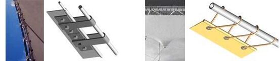
CONNECTING PLATE FOR STRUT AND MEMBRANE CONNECTION
CABLES
WOODEN STRUT
ETFE MEMBRANE
CONNECTING PLATE FOR STRUT AND MEMBRANE CONNECTION
95
FIG 5.28. Schematic diagram showing the rotation joint of the strut at the fixed end allowing 10 degrees of rotatory freedom.
FIG 5.30. Diagram showing cable and strut connection at the free end of the strut.
FIG 5.31. Diagram of ETFE membrane connection to the strut and the free strut end.
FIG 5.32. Image of the various connection apparatus used for connecing membrane to the strut and cables
FIG 5.29. Diagram of the end strut and cable joint at the fixed end.
STRUT FABRICATION
MODULEMODULESTRUT NUMBERSTRUT LENGTH (MM)TOTAL STRUTS
5A-S4,11.01S:526002600 X 5
(5 MODULES)S:142004200 X 5
S:342004200 X 5
S:260006000 X 5
S:460006000 X 5
5A-S4,11.01S:526002600 X 2 (2 MODULES)S:142004200 X 2
S:342004200 X 2
S:260006000 X 2
S:460006000 X 2
5C-S8,7.01(A)S:430003000 (1 MODULE)S:530003000
S:136003600
S:260006000
S:360006000
6A-S10,8.01(A)S:6900900 X 7 (7 MODULES)S:222002200 X 7
S:526002600 X 7
S:344004400 X 7
S:155005500 X 7
S:460006000 X 7
7E-S10,11.01(B)S:517001700 X 7 (7 MODULES)S:617001700 X 7
S:118001800 X 7
S:718001800 X 7
S:346004600 X 7
S:250005000 X 7
S:460006000 X 7
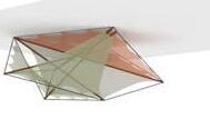
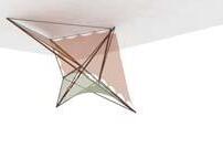
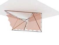
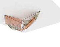
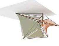
COMPONENT FABRICATION
In order to get an idea of the fabricati on costs and produc tion methods nd techniques, it was essential to quantify the design in terms of its elements and components required. This part of the study briefly lists down the various fabrication details required for the produc tion of the modules required on the test site. Based on the number of modules on the site, corresponding struts, cables and membranes required are listed as shown above, alongside and on the following page.
96
0 5 10 15 20 25 30 35 900 1700 1800 2200 2600 3000 3600 4200 4400 4600 5000 5500 6000 STRUT NUMBER / LENGTH FINAL STRUT LENGTHSNUMBER 9007 170014 180014 22007 260014 30002 36001 420014 44007 46007 50007 55007 600030
CABLE FABRICATION
5A-S4,11.01EC:43030 X 5 (5 MODULES)EC:3200200 X 5
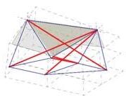
EC:1119001900 X 5
EC:919001900 X 5
EC:224002400 X 5
EC:1024002400 X 5
NEC:326002600 X 5
EC:126002600 X 5
EC:728002800 X 5
EC:533003300 X 5
EC:633003300 X 5
EC:840004000 X 5
NEC:142004200 X 5
NEC:242004200 X 5
NEC:442004200 X 5
5A-S4,11.01EC:43030 X 2
(2 MODULES)EC:3200200 X 2
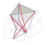
EC:1119001900 X 2
EC:919001900 X 2
EC:224002400 X 2
EC:1024002400 X 2
NEC:326002600 X 2
EC:126002600 X 2
EC:728002800 X 2
EC:533003300 X 2
EC:633003300 X 2
EC:840004000 X 2
NEC:142004200 X 2
NEC:242004200 X 2
NEC:442004200 X 2
5C-S8,7.01(A)EC:6600600
(1 MODULE)EC:514001400
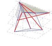
EC:720002000
EC:420002000
EC:320002000
EC:228002800
EC:128002800
NEC:129002900
NEC:629002900
NEC:430003000
NEC:547004700
NEC:847004700
NEC:347004700
NEC:748004800
NEC:248004800
6A-S10,8.01(A)EC:2900900 X 7 (7 MODULES)NEC:316001600 X 7
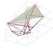
EC:117001700 X 7
NEC:522002200 X 7
NEC:922002200 X 7
EC:322002200 X 7
NEC:125002500 X 7
EC:530003000 X 7
EC:730003000 X 7
EC:637003700 X 7
NEC:438003800 X 7
NEC:238003800 X 7
NEC:740004000 X 7
NEC:840004000 X 7
EC:844004400 X 7
NEC:1044004400 X 7
NEC:644004400 X 7
EC:454005400 X 7
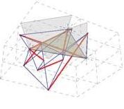
7E-S10,11.01(B)NEC:800 X 7 (7 MODULES)EC:10400400 X 7
EC:112001200 X 7
NEC:516001600 X 7
NEC:916001600 X 7
EC:317001700 X 7
NEC:418001800 X 7
EC:920002000 X 7
EC:521002100 X 7
EC:1122002200 X 7
EC:424002400 X 7
NEC:130003000 X 7
NEC:330003000 X 7
NEC:1030003000 X 7
EC:832003200 X 7
EC:632003200 X 7
NEC:735003500 X 7
NEC:637003700 X 7
NEC:238003800 X 7
EC:742004200 X 7
EC:242004200 X 7
97 0 5 10 15 20 25 30 35 40 30 400 900 1400 1700 1900 2100 2400 2600 2900 3200 3500 3800 4200 4700 5400 STRUT NUMBER / LENGTH FINAL CABLE LENGTHSNUMBER FINAL CABLE LENGTHSNUMBER 30725007 2007260014 400728009 600129002 9007300036 12007320014 14001330014 16002135007 170014370014 18007380021 190014400021
NUMBERCABLE LENGTH
TOTAL CABLE
200010420035 21007440021 22002847003 24002148002 2500754007 MODULEMODULECABLE
(MM)
MODULEMODULECABLE NUMBERCABLE LENGTH (MM) TOTAL CABLE
MEMBRANE FABRICATION
MODULEMODULE
5A-S4,11.01M14678622339310 (1-8-10)M2726714336335715
(5 MODULES)M3257495712874785

M4566537928326895 79876705
5A-S4,11.01M1539522810790456 (2-4-8)M243193088638616
(2 MODULES)M3633592412671848
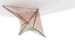
M4618044012360880
M5607011612140232 56602032
5C-S8,7.01(A)M188389758838975 (6-7-8)M226954832695483
(1 MODULE)M381667678166767
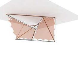
M480750818075081 27776306
6A-S10,8.01(A)M1522071236544984 (1-2-3)M212813148969198
(7 MODULES)M3261423018299610

M49437946606558
M5682184847752936 118173286
7E-S10,11.01(B)M1226951615886612 (6-9-12)M2666999746689979
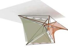
(7 MODULES)M35197733638411
M4234728816431016
M5637172144602047
M6364297625500832
M7261924618334722 171083619
98
MEMBRANE NO MEMBRANE AREA (MM2 ) TOTAL AREA (MM2 )
MECHANICAL PROPERTIES OF STRUCTURAL MEMBRANES STRUCTURE FIBERCOATINGDURABILITY (YEARS)WEIGHT (kg/m2)TENSILE STRENGTH (KN/5cm) POLYESTERPVC15-200.6-1.652.0-10.0 GLASSPTFE>250.4-1.61.0-8.0 ETFE(
foil)NONE>250.05-2.00.3-0.6
ourploymer
COMPONENT FABRICATION
In order to get an idea of the fabricati on costs and produc tion methods nd techniques, it was essential to quantify the design in terms of its elements and components required. This part of the study briefly lists down the various fabrication details required for the produc tion of the modules required on the test site. Based on the number of modules on the site, corresponding struts, cables and membranes required are listed as shown above, alongside and on the following page.
COST AND ASSEMBLY
ASSEMBLY PROCESS
PREFABRICATED STRUTS(FACTORY)
PRE SITE STRUTS (FACTORY) PROCESS
PRESTRESSED CABLES (FACTORY AND WORKSHOPS)
PRE FABRICATED MEMBRANESASPER MEMBRANES AS PER DESIGN REQUIREMENTS (FACTORY)
ONSITE
CONNECTION ASSEMBLY ON GROUND ON SITE PROCESS
MODULE ERECTION WIT CONNECTION OF CONNCTIONOFFINAFINAL STRUT INSTALLATION OF MEMBRANES
POST ASSEMBLY TIMELY DEPLOYMENT AND RE INSTALLATION BYUSERS BY USERS
99
100
CONCLUSION
01 LEARNINGS System Process Design
02 LIMITATIONS Process Methods
03 FURTHER SCOPE System Process Design
101 CHAPTER 06.
LEARNINGS
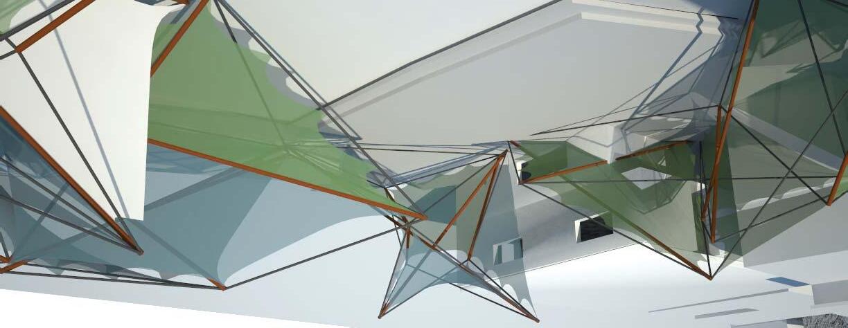
SYSTEM
The primary goal of designing program based Dynamic Tensegrity Structures was fairly achieved, especially at a digital level. The use of analy tical interfaces and generative tools provide a wide theoretical base for the design, exploration and development of the achieving Dynamism in Irregular Tensegrity Modules.
PROCESS
The use of digital scripting tools to predict structural behavior and formulate the algorithmic form-finding process helped in exploring the vast design space domain of Irregular Tensegrity Structures which has been very sparsely explored. The intense evaluation stages and elimination process helped in efficiently filtering out the potentially usable design modules. Simulation of non-linear complex system behavior, and the multiple-stable state result of the generative process successfully provides a digital apparatus for further studying, analyzing Irregular Tensegrity Structures including its varied application possibili ties.
DESIGN APPLICATION
Testing the system on a site context helped in understanding one of the architectural applications by designing use and user based dynamic flexible system that demonstrated deployability and mul tiplicity.
102
SYSTEM
The primary goal of designing program based Dynamic Tensegrity Structures was fairly achieved, especially at a digital level. The use of analy tical interfaces and generative tools provide a wide theoretical base for the design, exploration and development of the achieving Dynamism in Irregular Tensegrity Modules.
PROCESS
There was lack of a feed-back loop in the digital exploration which would enable the learnings and conclusions of each stage to be applied in the process by re-iterating the stages with revised procedures. The lack of application of the conclusions from the physical explorations and experiments in the generative algorithm was one of the major draw-back of the process followed. This however, is also due to the tedious nature of making Irregular physical models making exploratory process di fficult to follow. The process needed to be revised, this time by incorporating the physical experiments in form-finding and analysis stages.
DESIGN APPLICATION
The system was tested on only of the program applications, which was habilitating the rapidly growing informal slum settlements in large dense urban areas. The application on a site like Mumbai has certain construc tion concerns of lack of technology for fabrication, installation and assembly of modules in dense sites.
LIMITATIONS
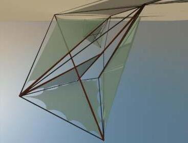
103
SYSTEM
Combining the system with springs or sensors would further investigate the dynamic system behavior without the need to mechanically change the structure. There is also further scope of researching on methods and techniques that would explore the modularity of the system in much deeper sense to come up with more emerging complex structural systems.
PROCESS
Designing a feedback loop in the generative process with intense evaluation criteria would result in better, faster optimum results. In addi tion to this, there is a scope of developing this generative algorithmic process into an evaluative evolu tionary algorithm, that would give a more optimized result through higher intensive methods.
DESIGN APPLICATION
Exploring structure and organization at a further complex level of mul tistorey structures would widen the application of the system.
104
FURTHER SCOPE
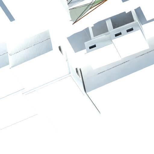
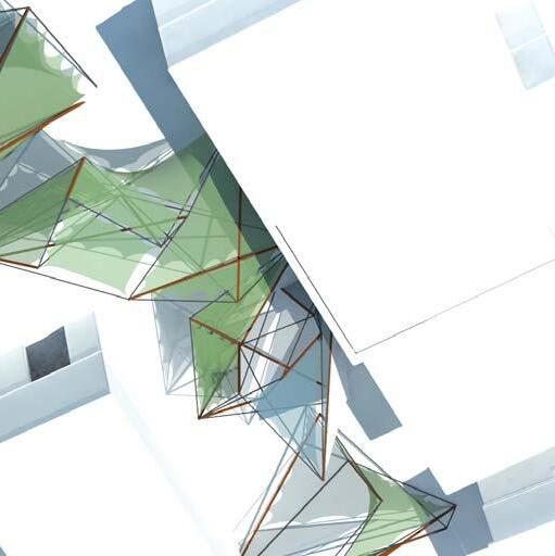

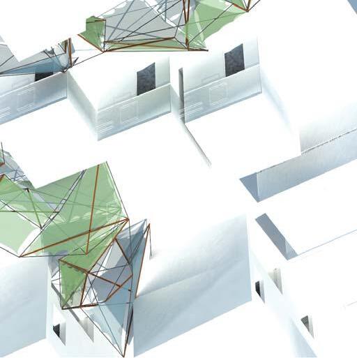
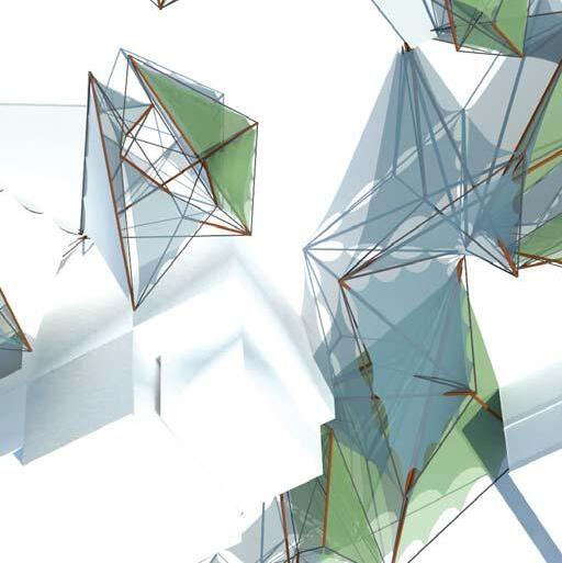
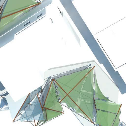
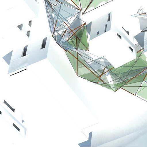
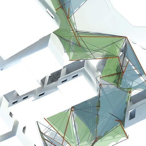
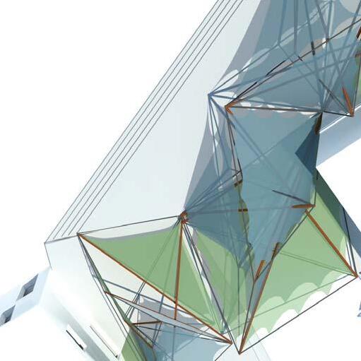
105
106
01 SYSTEM AND METHODS
History
Defini tions
Classi fication
Analy tical Methods
Mathematical Concepts (Lipson)
03 PHYSICAL EXPERIMENTS
Regular Morphologies
Irregular Morphologies
Random Morphologies
Modules
Membranes
03 DIGITAL EXPERIMENTS AND ANALYSIS
Grasshopper Parametric Exploration
Detailed Pseudo-code
Generative Script
Morphology Generation
Evaluation Stage 1
Evaluation Stage 2
Module Strand Analysis
Module Orientation Catalogue
Membrane Enclosures
Membrane Strand Analysis
04 DESIGN AND DETAIL
Site Studies
Typology Studies
Fabrication Examples
APPENDIX
107
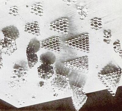
http://chemoton.wordpress.com/2009/07/03/tensegrity
BACKGROUND
Until the last century, the technique of construc tion and the philosophy of building have been very simple with everything being held in place by weight, so the continui ties of stress were basically compressive. Tensegrity structures are based on a quite an inverse concept wherein instead of the “weight and support” strategy, a “system of equilibrated omni-direc tional stresses” is integrated. Furthermore, the system need not be supported as it is self-equilibrated and pre-stressed, thus independent of gravitational forces for equilibrium.
Tensegrities are spatial, reticulated and lightweight structures that basically consist of isolated compression members (rigid bars) suspended by a continuous network of tension members (cables). These highly intriguing structures, especially for their unique visual quali ties and
topological characteristics, were first developed by artist Kenneth Snelson in 1948 as well as independently by David Emmerich. Buckminster Fuller further developed Tensegrity structures from Snelson’s ideas by applying engineering principles to the study. He also coined the term Tensegrity from “tensile integrity” as the integrity or stability of the system comes from the tension members. As implied by their name, Tensegrity structures to dynamic loading and exhibit non-linear behavior.
ANALOGIES
The most primi tive and simple case of stressed structures is the kite. This antique toy is simply based on two crossed sticks with a tensioned string around it, joining the four extremes defined by them. Snelson achieved his first Tensegrity sculpture from kite-like modules out of plywood. One of the most common analogies has been the comparison between
108 HISTORY
DEFINITIONS
DEFINITIONS AND PATENTS
Buckminster Fuller, in 1962, in his patent, describes Tensegrity structures (tensional-integrity systems) as “a plurality of discontinuous compression columns arranged in groups of three non-conjunctive columns connected by tension elements forming tension triangles”.
David G. Emmerich , declared in his patent that his invention could be further described in a non-limita tive manner with reference to several examples.
Kenneth Snelson, in 2004, described Tensegrity Structures or the “floating compression structures”, as he called them, as “ Tensegrity describes a closed structural system composed of a set of three or more elongate compression struts within a network of tension tendons, the combined parts mutually suppor tive in such a way that the struts do not touch one another, but press outwardly against nodal points in the tension network to form a firm, triangulated, prestressed, tension and compression unit. ”
Anthony Pugh, in 1976, gave the almost universally accepted characterization: “A Tensegrity system is established when a set of discontinuous compressive components interacts with a set of continuous tensile components to define a stable volume in space.”
Schodeck, in 1993, defined Tensegrities based on redundancies and degrees of freedom as “rigid structures made of discontinuous rods in compression and continuous cords in tension in which each component has one degree of member redundancy.”
Bin-Bing Wang, in 1998 identified that the Tensegrity structures are selfsuppor ting and rigidi fied by self-stressing and gave a wider defini tion: “Tensegrity systems are free-standing pin-jointed cable networks in which a connected system of cables are stressed against a disconnected system of struts and extensively, any free-standing pin-jointed cable networks composed of building units that sa tisfiy aforesaid definition.”
Kanchanasaratool and Williamson, in 2002, stated that a Tensegrity system is a stable connec tion of axially-loaded members, being a Class k Tensegrity structure if at most “k” compressive members are connected to any node. E.g., a tradi tional Tensegrity structure is a class 1 structure because only one compression member makes a node.
Ariel Hanaor described Tensegrity structures as “internally prestressed, free-standing pin-jointed networks, in which the cables or tendons are tensioned against a system of bars or struts” .
Miura and Pellegrino, in 2002, gave a narrower interpretation: “A Tensegrity structure is any structure realized from cables and struts, to which a state of prestress is imposed that imparts tension to all cables”, adding later, “the state of prestress serves the purpose of stabilizing the structure, thus providing first-order stiffness to its in finitesimal mechanisms.”
René Motro, in 2003 tried to distinguish two di fferent concepts. He makes the distinction between the “patent based” and the “extended” defini tion. Patent based defini tion is “ Tensegrity systems are spa tial reticulate systems in a state of self-stress. All their elements have a straight middle fibre and are of equivalent size. Tensioned elements have no rigidity in compression and constitute a continuous set. Compressed elements constitute a discontinuous set. Each node receives one and only one compressed element.” While the extended defini tion is “Tensegrity system is a system in a stable self-equilibrated state comprising a discontinuous set of compressed components inside a continuum of tensioned components.”
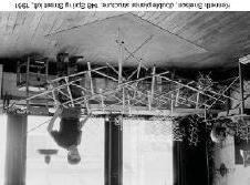
109
CLASSIFICATION
CONNECTION BASED:
A. Tensegrity
B. Geodesic
MORPHOLOGY BASED:
The concern of form-finding is central in the study of Tensegrity structures and thus it becomes highly essential to understand this system and classifying based on its morphology. Tensegrity structures exhibit system behavior at various progressive levels ranging from simple cell simplex structure level to a more complex assembly level. Hence the first stage of classi fication would be on the basis of organizational criteria of being single morphology modules or hierarchically organized assemblies of simpler modules.
A. Single Morphologies
B. Assemblies
A. SINGLE MORPHOLOGIES
Single Tensegrity modules are essentially individual independent selfstressing stable arrangements of compressive and tensile components that balance out the forces and nodal stresses to establish equilibrium in space. The next level of classification of these single modules is based on the parametric properties of the components and the connec tion pattern resulting in Regular and Irregular morphologies.
1. Regular Morphologies
Regular Tensegrity structures inherently have same component parameters like strut length, cable lengths, connection patterns and rotation angle. Regular Tensegrity structures have been extensively studied, researched and analyzed in the field of Tensegrity structures. These regular structures can be further classified based on number of struts connecting at each node. A Tensegrity structure is classi fied as a structure of class ‘k’ when I has k number of struts connec ting at each node.
i. Class 1
Class 1 Tensegrity structures essentially have only one strut connec ting at each node and at least 3 cables balancing out the compressive strut forces by their tensile pull.
a. X-shape:
The basic idea developed by Snelson was contained in X-shape which is an assembly of two struts and four cables the whole system being in self equilibrium.
b. Prismatic Regular Tensegrity Cells:
The class of prismatic Tensegrity structures is defi ned as structures with n number of same length struts resul ting in 2n number nodes arranged in 2 horizontal circles around + z axis, which is an n-fold symmetry axis. Within each circle, each node is connected to two other by horizontal cables and each node is connected diagonally to node in other planar circle by a strut and verticle cable.
c. Tensy-Polyhedra
Tensy-polyhedra geometries are basically developed by inserting struts inside regular polyhedron geometry to establish self stress state of equilibrium. David Emmerich used this form finding method to develop and design Tensegrity cells from regular polyhedron geometries. It was discovered that some geometries are stable while others are essentially unstable forms. Icosahedrons, expanded octahedrons and truncated tetrahedrons are standard examples of regular tensy-polyhedra structures.
ii. Class 2
Class 2 Tensegrity structures essentially have 2 struts connec ting at each node and at least 4 cables balancing out the compressive struts forces by their tensile pull.
a. Tensegrity circuits
These systems are characterized by its compoenets which are no longer single struts but chain of struts. Cuboctahedron and Mono-circuit tensypolyhedron are good examples of these systems. The former geometry has triangular compressed components (each constituting a chain of strut) with a hexagon of tensile cables maintaining the equilibrium.
110
B. ASSEMBLIES
1. Regular Assemblies
i. Class 1
a. Double-x , Triple-x:
Kenneth Snelson developed his X-shape modules further by assembling more than one to form Double-X and Triple-X shaped sculptures.
b. Tensegrity towers:
Tensegrity towers are vertical modular structures of simple prismatic Tensegrity modules assembled and arranged vertically with alternate clockwise and anticlockwise rotation of the module. Snelson’s needle tower is one good example of a built Tensegrity tower sculptures.
c. Tensegrity cloud:
The first attempt at developing complex systems based on changing parameters from regular components to multi-parameter systems was undertaken by Nicolas Vassart mainly concerning with cytoskeletons in biology. As the exploration was di fficult digitally, it was experimented in terms of physical models to develop final form.
ii. Class 2
a. Tensegrity rings
Anthony Pugh experimented with these assemblies where the formal development evolved from using symmetric prismatic structures following a certain process resulting into hollow tube shaped Tensegrity cells called the Tensegrity rings. The foldability and deployability of these structures make them essentially useful for temporary structures.
111
ANALYTICAL METHODS
INTRODUCTION
A key step in the design of tensegrity structures is the determination of their geometrical configuration, known as form-finding. Early studies by Fuller, Snelson and Emmerich into the form of tensegrity structures used mainly regular, convex polyhedra as the basis for finding new configurations.
KINEMATICAL METHODS:
The characteristic of these methods is that the lengths of the cables are kept constant while the strut lengths are increased until a maximum is reached. Alternatively, the strut lengths may be kept constant while the cable lengths are decreased until they reach a minimum. This approach mimics the way in which tensegrity structures are built in prac tice, without explicitly requiring that the cables be put in a state of pre-tension. However, physical models of these structures showed that proper formfinding methods are needed to find the equilibrium configuration of even the simplest tensegrity structure. The methods explored by various researchers can be broadly classified into:
A. Kinematical Methods
B. Statistical Methods
A. KINEMATICAL METHODS
The characteristic of these methods is that the lengths of the cables are kept constant while the strut lengths are increased until a maximum is reached. Alternatively, the strut lengths may be kept constant while the cable lengths are decreased until they reach a minimum. This approach mimics the way in which tensegrity structures are built in prac tice, without explicitly requiring that the cables be put in a state of pre-tension.
1. Analy tical Solutions
A compact description of the geometry of this problem, taking advantage of its symmetry, was introduced by Connelly and Terrell, as follows. In the starting configuration the lateral cable, 1 2, is vertical and the angle between the ends of the strut is 2 πj/v where j is an integer smaller than v. The coordinates of nodes 1–5 are:
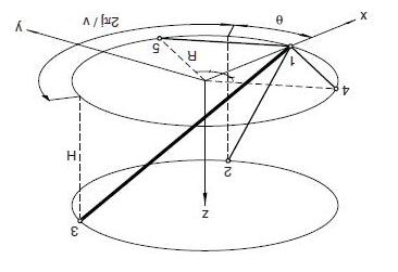
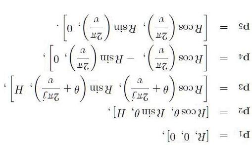
2. Non-Linear Programming
This general method, proposed by Pellegrino, turns the form-finding of any tensegrity structure into a constrained minimisation problem. Star ting from a system for which the element connectivity and nodal coordinates are known, one or more struts are elongated, maintaining fixed length ratios, until a configuration is reached in which their length is maximised. The general constrained minimisation problem has the form:
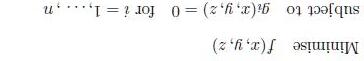
where the objective function f(x, y, z) is, for example, the negative length of one of the struts. Pellegrino applied this method to two tensegri ties: the triangular prism and the truncated tetrahedron.
3. Dynamic Relaxation
The Dynamic Relaxation method has good convergence proper ties for structures with only a few nodes but is not effective when the number of nodes increases. Also, the method becomes rather cumbersome if several different ratios between strut lengths and cable lengths are desired, which restricts its applicability to less regular structural forms. For a structure in a given ini tial configuration and subject to given external forces the equilibrium of configuration can be computed by integrating the following fictitious dynamic equations
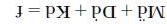
Where K is a stiffness matrix, M a mass matrix, D a damping matrix, f the vector of external forces, and ¨d, ˙d and d the vectors of acceleration, velocity and displacement from the ini tial configuration, respectively. Both M and D are taken to be diagonal, for simplicity, and the veloci ties and displacements are ini tially set to zero.
B. KINEMATICAL METHODS
The general characteristic of these methods is that a relationship is set up between equilibrium configurations of a structure with given topology and the forces in its members. This relationship is then analysed by various methods.
1. Analy tical Solutions
Kenner used node equilibrium and symmetry arguments to find the configuration of the expandable octahedron, whose six identical struts are divided into three pairs and the distance between the struts in each pair is exactly half the strut length. Other, more complex, spherical tensegrities with polyhedral geometries, i.e. the cuboctahedron and the icosidodecahedron, were also analyzed using the same approach.
112
Denoti ng by qij the force density in element ij —note that q1,4 = q1,5 due to symmetry— the equilibrium of node 1 in the z- and y-direc tion can be written as
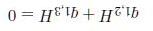
2. Force Density Method
The force density method for cable structures, first proposed by Linkwitz and Schek in 1971, uses a simple mathematical trick to transform the nonlinear equilibrium equations of the nodes into a set of linear equations. For example, the equilibrium equation in the x-direc tion for node i is
3. Energy Method
Connelly and Back have analysed tensegrity structures with di fferent types of symmetry using this method. Their ini tial assumption was that there is a symmetric state of self-stress with a force density of 1 in each cable and −ω s in each strut. A further assumption was that there are two types of cables but only one type of strut, arranged such that satisfying equilibrium at only one node of the structure implies, by symmetry, that it is satisfied also at all other nodes. The force density in the strut is chosen such that the structure is super stable. A complete catalogue of all the tensegrity structures that are possible for each symmetry group has been produced, using group theory. Although some of the systems in the catalogue have struts that go through each other, and therefore are of limited prac tical interest, the catalogue contains many solu tions that were previously unknown. In analogy with the total potential energy, defines the following energy form associated with the stress ω:
4. Reduced Coordinates
This method was introduced by Sultan. Consider a tensegrity structure whose b elements consist of M cables and O struts. The struts are considered as a set of bilateral constraints ac ting on the cable structure. Hence, a set of independent, generalized coordinates g = [g1, g2, . . . , gN]T is defined, which define the posi tion and orientation of these struts.
113
MATHEMATICAL THEORY
THE BASIC RELAXATION PROCESS FOR STATIC STRUCTURES
The basic relaxation process, as applied to pin-joined structures, comprises two steps applied iteratively. The first step computes the total net force Ri on each joint; this is the residual force, since these forces should be zero if the structure is in perfect equilibrium. The second step adjusts the posi tion vector xi of each joint so as to reduce the residual force acting upon it. These two steps are repeated until the maximum residual force goes below a desired threshold. The residual force vector Ri acting on joint i is computed by summing all the forces produced by links connected to it
where Li is the set of all links meeting at joint i, lj is the current length of link j, lj=xj2 xiand j2 is the index of the other joint to which link j is connected, l0j is the given nominal length of link j, xi is a vector of the coordinate of joint i, kj is the stiffness of link j, e.g., for a beam kj=EjAj / lj where E is the modulus and A is the cross section area<?>, nˆ j is the unit vector in the direc tion of the link nˆ j=xj2 xi<?> / xj2 xi , and Fi is any external force vector ac ting on joint i e.g. gravity<?>.
The effective stiffness vector Si of each joint i is estimated by summing all the stiffness of all links connected to it
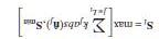
where absnj<?> is a unit vector composed of the absolute value of each term in the unit vector in the direc tion of the link, absnˆ j<?> =nˆ x , nˆ y , nˆ z . Note that to handle singulari ties, Si must be ensured to be nonzero by not allowing it to go below Smin see the next sec tion for a discussion of singulari ties<?>. Given the residual force ac ting on each joint and its effective stiffness, the displacement vector i of joint i is computed as the ratio where is a relaxation factor typically in the range 01 but occasionally larger over-relaxation<?>. The displacement can be capped by some value max. The joint positions of ungrounded nodes only<?> are then updated by
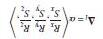
Equations 1<?>–4<?> are repeated until the overall largest residual force maxRi<?> goes below a desired threshold <?>. Grounded nodes are omitted from this maximum.
The steps above are aggregated in the pseudocode shown below. For greater computational efficiency, many of the above steps can be calculated concurrently using the pseudocode shown , resul ting in faster performance but in some cases loosing guarantees on convergence. In practice, the relaxation factor is o ften gradually reduced from a large number ini tially
e.g., 0.5<?> to a small number e.g., 0.01<?> as the residuals diminish. This relaxation schedule may need to be adjusted dynamically for some stable structures.
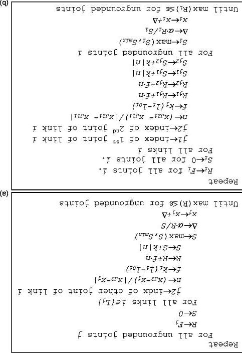
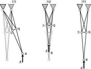
114
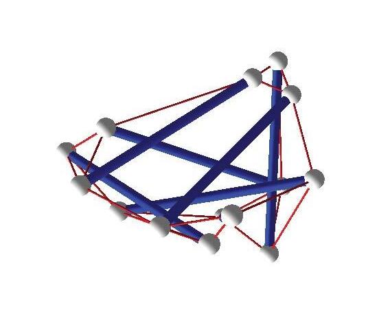
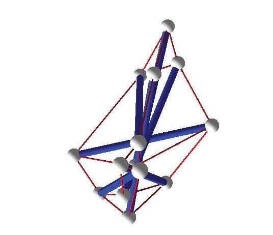
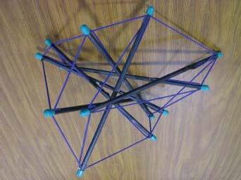
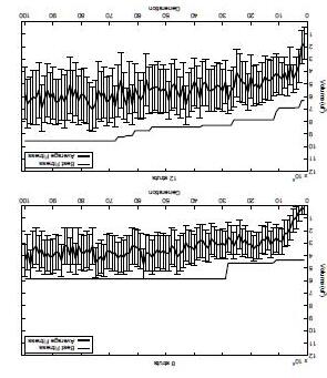
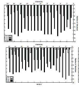
115
PHYSICAL EXPERIMENTS
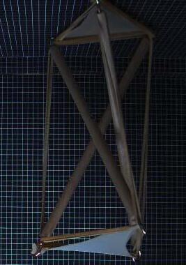
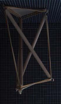
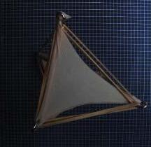
PRELIMINARY PHYSICAL EXPERIMENTS
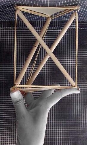
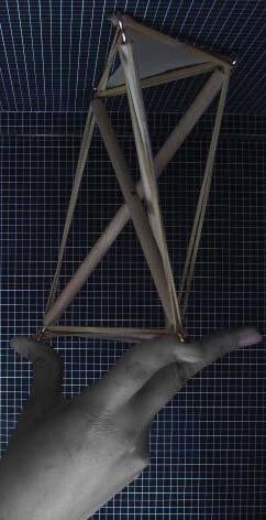
116
3 strut Tensegrity Model
3 strut Tensegrity Model tested for deformation
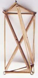
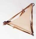
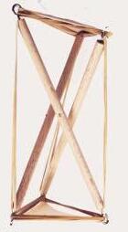
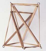
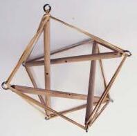
3 strut Tensegrity Model
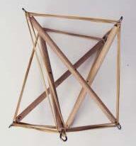
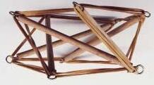
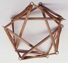
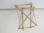
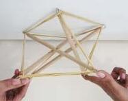
4 strut Regular Tensegrity
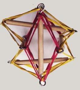
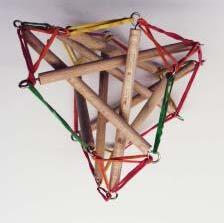
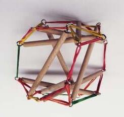
9 strut regular tensegrity tet-
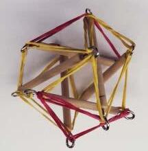
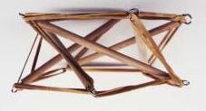
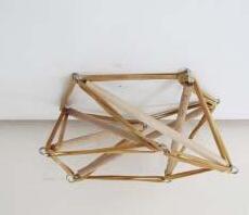
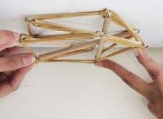
5 strut Regular Tensegrity Model tested for deformation
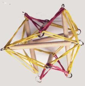
6 strut regular tensegrity
117
REGULAR MORPHOLOGIES
Model tested for deformation
rahedron
model
IRREGULAR MORPHOLOGIES
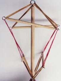
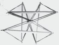
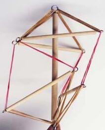
5 Strut Irregular tensegrity model with its mul tiple stable state.
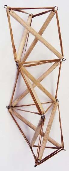
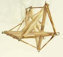
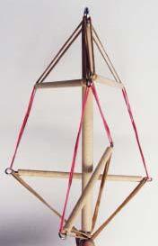
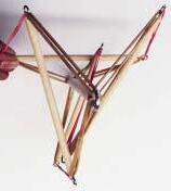
3 tiered Tensegrity tower of 3 strut tensegrity modules.
5 Strut Irregular tensegrity model with its mul tiple stable state.
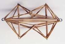
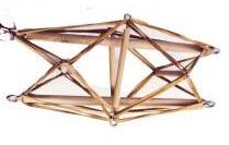
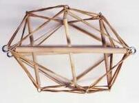
6 strut irregular tensegrity module
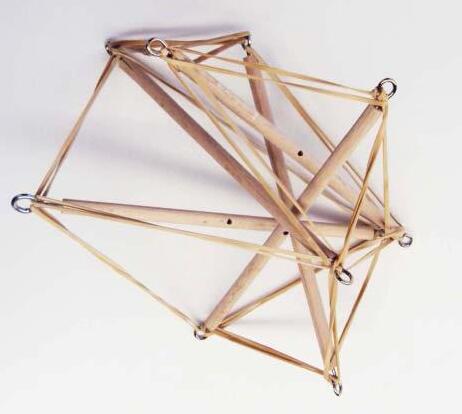
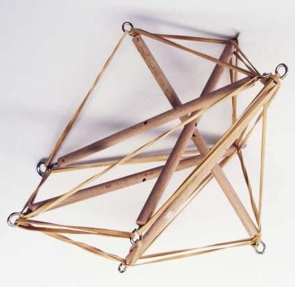
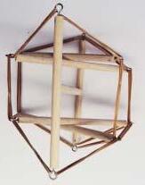
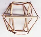
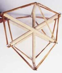
5 Strut Irregular tensegrity model
118
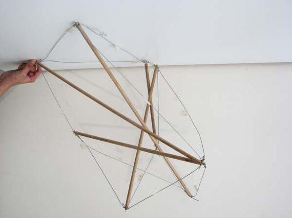
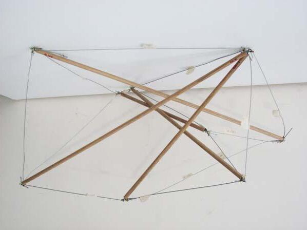
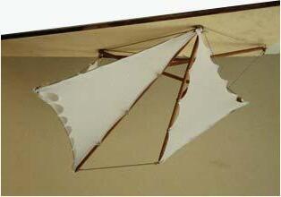
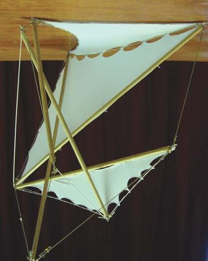
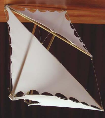
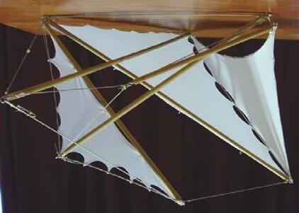
119
MODULES
Stable model for the 5 strut selected module.
GRASSHOPPER PARAMETRIC EXPERIMENT
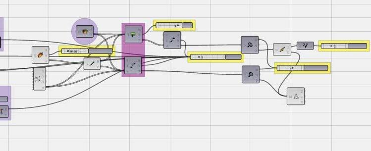
Grasshopper defini tion for the alongside given variation in geometry.
120
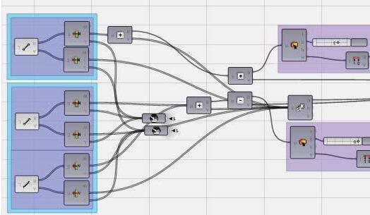
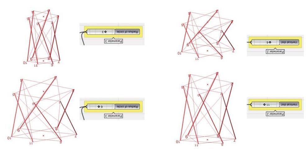
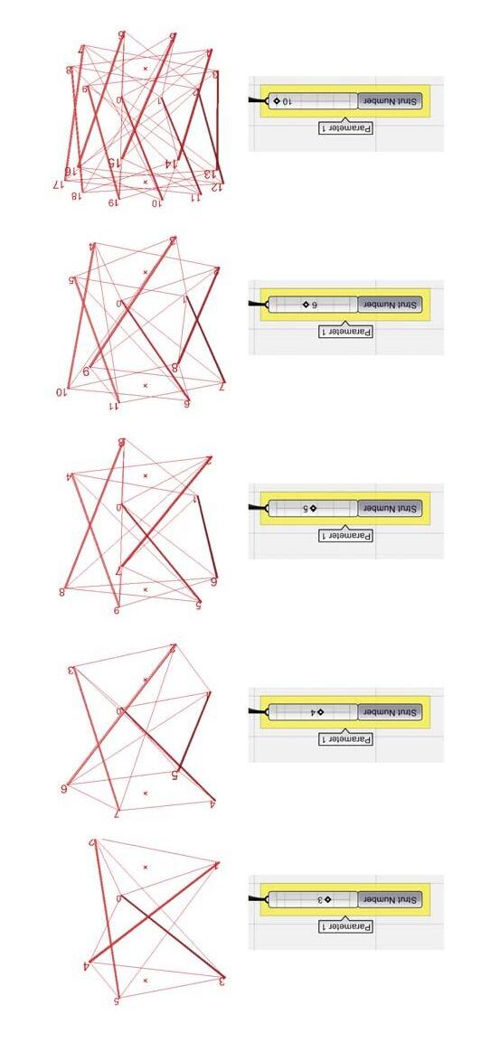
121
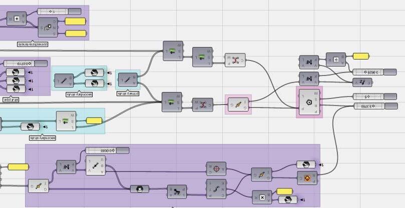
Grasshopper defini tion for the alongside given variation in geometry.
122
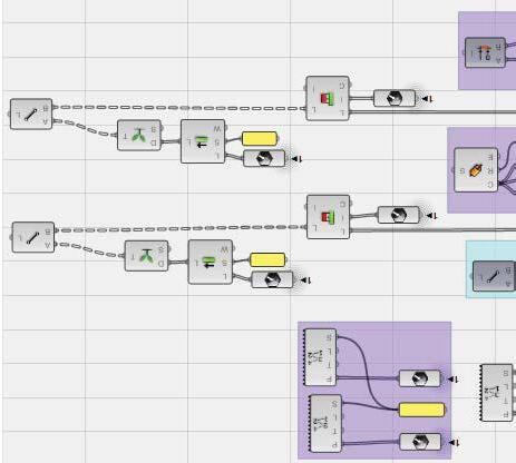
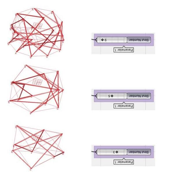
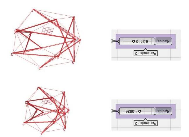
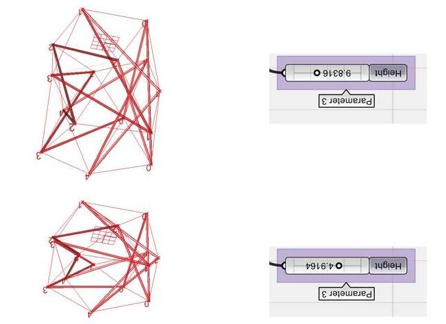
123
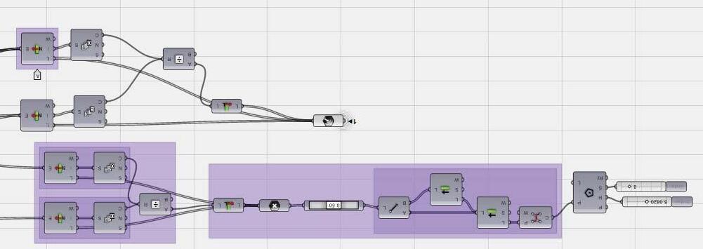
Grasshopper defini tion for the alongside given variation in geometry.
124
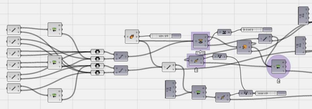
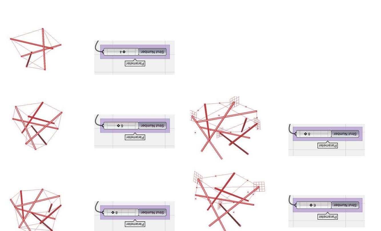
125
DETAILED PSUEDO-CODE
GENOME WRITING:
MAKING POINTS
(each vertex connected to next 2
MAKING LINKS
CONVERTING LINKS TO STRUTS AND CABLES
MAKING STRUTS
SHUFFLING OF CABLES AND STRUTS TO OBTAIN RANDOM GEOMETRY
126
-
CALCULATING NODAL FORCES
127
--
DYNAMIC RELAXATION
GENERATIVE ALGORITHMIC SCRIPT
Rhino- Script
Option Explicit
‘Script written by <Dishita>
‘Script copyrighted by <Dishita>
‘Script version Monday, June 28, 2010 6:03:10 PM
Call Main() Sub Main()
‘G E N O M E W R I
‘MAKING POINTS:____________________
Dim n ‘n = number of struts n = rhino.GetInteger (“enter number of struts”)
Dim arrVertices:arrVertices = GeneratePoints(n)
‘ MAKING LINKS:______________________
Call rhino.AddLayer(“Links”,RGB(255, 0, 0))
Dim links(), line1, line2,arrLinks
Dim j
Dim x:x=ubound(arrVertices)
ReDim arrLinks(x,x)’ this is to check overlap of links later
Call rhino.CurrentLayer (“Links”)
For j = 0 To ((2*n)-1)
If j < ((2*n)-2) Then line1 = rhino.AddLine(arrVertices (j),arrVertices (j+1))
arrLinks((j),(j+1)) = line1
line2 = rhino.AddLine(arrVertices (j),arrVertices (j+2))
arrLinks((j),(j+2)) = line2
ElseIf j = ((2*n)-2) Then line1 = rhino.AddLine(arrVertices (j),arrVertices (j+1))
arrLinks((j),(j+1)) = line1
line2 = rhino.AddLine(arrVertices (j),arrVertices (0))
arrLinks((j),(0)) = line2
ElseIf j = ((2*n)-1) Then line1 = rhino.AddLine(arrVertices (j),arrVertices (0))
arrLinks((j),(0)) = line1
line2 = rhino.AddLine(arrVertices (j),arrVertices (1))
arrLinks((j),(1)) = line2
End If
ReDim Preserve links(2*j) links(2*j) = line1
ReDim Preserve links((2*j)+1) links((2*j)+1)= line2
Next
‘MAKING STRUTS ARRAY:________________________________
Dim struts ()
ReDim struts (n-1)
Dim m, PipeRad
Piperad = 0.025
For m = 0 To (n-1)
struts (m)= links (4*m)
Next
‘MAKING CABLES ARRAY:________________________________
Dim cables (), p
ReDim cables ((3*n)-1)
For p = 0 To (n-1)
cables (3*p)= links ((4*p)+1)
cables ((3*p)+1)= links ((4*p)+2)
cables ((3*p)+2)= links ((4*p)+3)
Next
‘SHUFFLING STRUTS: MUTATION1___________
Dim Sx, Sy, l
Dim arrMutation1 ()’number of times struts are shuffled
ReDim arrMutation1((2*n)-1)
Dim Sx1,Sx2,Sy1,Sy2
For = 0 To ((2*n)-1) Do
Sx = rhino.Floor((rnd()*(n-1))) Sy = rhino.Floor((rnd()*(n-1))) ‘Sx, Sy are the random pair of struts to be shuffled ‘to prevent overlap
Sx1 = rhino.CurveStartPoint(Struts(Sx))
Sx2 = rhino.CurveEndPoint(Struts(Sx))
Sy1 = rhino.CurveStartPoint(Struts(Sy))
Sy2 = rhino.CurveEndPoint(Struts(Sy))
Dim CheckSx1,y1 Do
For y1 = 0 To x Checksx1 = rhino.PointCompare(arrVertices(y1),Sx1) If (CheckSx1) Then Exit Do Next Loop
Dim CheckSx2,y2 Do For y2 = 0 To x CheckSx2 = rhino.PointCompare(arrVertices(y2),Sx2) If (CheckSx2) Then Exit Do Next Loop
Dim CheckSy1,y3 Do For y3 = 0 To x CheckSy1 = rhino.PointCompare(arrVertices(y3),Sy1) If (CheckSy1) Then Exit Do Next
Loop
Dim CheckSy2,y4
Do For y4 = 0 To x CheckSy2 = rhino.PointCompare(arrVer ti ces(y4),Sy2)
If (CheckSy2) Then Exit Do Next Loop
Dim checkline1,checkline2 checkline1 = (rhino.IsLine(CStr (arrLinks((y1),(y4))))) If isNull(checkline1) Then checkline1 = False
checkline2 = (rhino.IsLine(CStr (arrLinks((y3),(y2))))) If isNull(checkline2) Then checkline2 = False
If Sx <> Sy And (Not(checkline1))And (Not(checkline2)) Then Exit Do Loop
128
N G : - - - - - - - - - - - - -- - - -- - - -- - - - -- - - - - - - - - - - - - - - -
T
Call rhino.DeleteObjects(array(struts(Sx),Struts(Sy)))
arrLinks(y1,y2)= Empty
arrLinks(y3,y4)= Empty
Struts(Sx)= rhino.AddLine(Sx1,Sy2)
Struts(Sy)= rhino.AddLine(Sy1,Sx2)
arrLinks((y1),(y4))= Struts(Sx)
arrLinks((y3),(y2))= Struts(Sy)
‘ to store the changing strut names and the end points that are interchanged arrMutation1(l) = array(Sx,Sy,Sx2,Sy2) Next
‘CONSTRUCTION OF ALL STRUTS:____________________________
Call rhino.AddLayer(“Struts”,RGB(0,255, 233))
Call rhino.CurrentLayer (“Struts”)
Call StrutAll (struts,n,PipeRad)
Call rhino.CurrentLayer (“Links”)
‘SHUFFLING CABLES: MUTATION2___________________________
Dim arrMutation2 ()’Number of times Cables are shuffled
Dim NoIteration
‘as Number of Iteration = twice number of cables
‘Number of cables = 3*n ‘NoIteration = (2*(3*n))
NoIteration = (3*((2*n)-1))
ReDim arrMutation2((NoIteration)-1)
Dim q
For q = 0 To ((NoIteration)-1)
‘redim cables()
‘cables() = ShuffleCables(arrVertices,Cables,arrLinks,n,x)
‘Call ShuffleCables(arrVertices,Cables,arrLinks,n,x)
Dim Cx,Cy
Dim Cx1,Cx2,Cy1,Cy2
Do ‘this Do Loop checks that once shuffled, the lines dont end up as points
Cx = rhino.Floor((rnd()*((3*n)-1)))
Cy = rhino.Floor((rnd()*((3*n)-1)))
‘Cx, Cy are the random pair of cables to be shuffled ‘ make the above thing a functional loop later
Cx1 = rhino.CurveStartPoint(cables(Cx))
Cx2 = rhino.CurveEndPoint(cables(Cx))
Cy1 = rhino.CurveStartPoint(cables(Cy))
Cy2 = rhino.CurveEndPoint(cables(Cy))
Dim PtCompare1, PtCompare2, PtCompare3, PtCompare4
PtCompare1 = rhino.PointCompare (Cx1,Cy2)
PtCompare2 = rhino.PointCompare (Cx2,Cy1)
PtCompare3 = rhino.PointCompare (Cx1,Cy1)
PtCompare4 = rhino.PointCompare (Cx2,Cy2)
Dim CheckCx1,z1 Do For z1 = 0 To x CheckCx1 = rhino.PointCompare(arrVertices(z1),cx1)
If (CheckCx1) Then Exit Do Next Loop
Dim CheckCx2,z2 Do For z2 = 0 To x CheckCx2 = rhino.PointCompare(arrVertices(z2),Cx2) If (CheckCx2) Then Exit Do Next
Loop
Dim CheckCy1,z3 Do For z3 = 0 To x CheckCy1 = rhino.PointCompare(arrVertices(z3),Cy1) If (CheckCy1) Then Exit Do Next Loop
Dim CheckCy2,z4 Do For z4 = 0 To x CheckCy2 = rhino.PointCompare(arrVertices(z4),Cy2) If (CheckCy2) Then Exit Do Next
Loop
Dim checkline3, checkline4,checkline5,checkline6 checkline3 = (rhino.IsLine(CStr (arrLinks((z1),(z4))))) If isNull(checkline3) Then checkline3 = False checkline4 = (rhino.IsLine(CStr (arrLinks((z3),(z2))))) If isNull(checkline4) Then checkline4 = False
checkline5 = (rhino.IsLine(CStr (arrLinks((z4),(z1))))) If isNull(checkline5) Then checkline5 = False
checkline6 = (rhino.IsLine(CStr (arrLinks((z2),(z3))))) If isNull(checkline6) Then checkline6 = False
If Cx <> Cy And (Not (PtCompare1)) And (Not (PtCompare2)) And (Not (PtCompare3)) And (Not (PtCompare4)) And (Not(checkline3))And (Not(checkline4)) And (Not(checkline5))And (Not(checkline6)) Then Exit Do Loop
Call rhino.DeleteObjects(array(Cables(Cx),Cables(Cy))) arrLinks(z1,z2)= Empty arrLinks(z3,z4)= Empty
Cables(Cx)= rhino.AddLine(Cx1,Cy2) Cables(Cy)= rhino.AddLine(Cy1,Cx2) arrLinks((z1),(z4))= Cables(Cx) arrLinks((z3),(z2)) = Cables(Cy)
‘ShuffleCables = Cables arrMutation2(q) = array(Cx,Cy,Cx2,Cy2) Next
to store the changing strut names and the end points that are interchanged
final Genome:
Dim Genome
Genome = array(arrVertices,arrMutation1,arrMutation2)
129
‘RENAMING STRUTS AND CABLES BASED ON NODES:________________
Dim NodalStruts: Nodalstruts = RenameStruts(arrVertices,n,Struts)
Dim NodalCables: Nodalcables = RenameCables(arrVertices,n,Cables)
Dim NewPoints
Newpoints = arrVertices
Newpoints = NodalStiffness(arrVertices,n,NodalCables,NodalStruts)
Dim NewLinks
‘NewLinks = array(NewStruts,NewCables)
Newlinks = NewLinksDraw (arrVertices,newpoints,n,NodalStruts,NodalCables)
‘Call rhino.DeleteObjects(rhino.ObjectsByLayer(“Links”,True))
‘Call rhino.DeleteObjects(rhino.ObjectsByLayer(“Original Vertices”,True))
‘@@@@@@@@----Repeating Function----@@@@@@@@
‘later replace by RF value
Dim gen
For gen = 1 To 10 arrVertices = NewPoints
NodalStruts = Newlinks(0)
NodalCables = Newlinks(1)
Newpoints = NodalStiffness(arrVertices,n,NodalCables,NodalStruts)
Newlinks = NewLinksDraw (arrVertices,newpoints,n,NodalStruts,NodalCables)
Next
Call rhino.AddLayer(“Final Links”,RGB(0,0, 255))
Call rhino.CurrentLayer (“Final Links”)
End Sub
‘FUNCTION FOR GENERATING POINTS:_______________________________________________ Function GeneratePoints(ByVal n)
Dim arrVerticesPts () ReDim arrVerticesPts (2*(n)-1)
Dim RoughPt1, RoughPt2, centrePt, Scale Scale = 25
RoughPt1 = rhino.VectorScale((array (rnd(),rnd(),rnd())),Scale)
RoughPt2 = rhino.VectorScale((array (rnd(),rnd(),rnd())),Scale) centrePt = (rhino.VectorDivide(rhino.VectorSubtract(RoughPt1,RoughPt2),2))
Dim k, RotAngle, RotAxis
RotAngle = (360/n)
RotAxis = Rhino.VectorCreate (RoughPt1,RoughPt2)
Call rhino.AddLayer(“Original Vertices”,RGB(234, 145, 212))
Call rhino.CurrentLayer (“Original Vertices”)
For k = 0 To n-1 arrVerticesPts (k) = (rhino.PointCoordinates(Rhino.RotateObject(rhino.addpoint (Rough Pt1),centrePt,(k*RotAngle),RotAxis,True)))
arrVerticesPts (k+n) = (rhino.PointCoordinates(Rhino.RotateObject (rhino.AddPoint (Rou ghPt2),centrePt,(k*RotAngle),RotAxis,True)))
Next
GeneratePoints = arrVerticesPts
End Function
FUNCTION FOR ALL STRUTS PIPING:_______________________________________________
Function StrutAll (ByVal struts(), ByVal n, ByVal PipeRad)
Call rhino.CurrentLayer (“Struts”)
Dim i, Pipes()
For = 0 To n-1
Call StrutOne (struts(i), PipeRad) Next
End Function
FUNCTION FOR ONE STRUT PIPE:___________________________________________
Function StrutOne (ByVal curve, ByVal Rad)
Call rhino.CurrentLayer (“Struts”)
Dim strCmd, finalstrut strCmd = “! _-Pipe _SelID “ & curve & “ “ & Rad & “ _Cap=_Flat _Enter _Enter” Call Rhino.Command(strCmd, 0)
End Function
‘FUNCTION FOR SHUFFLING CABLES:______________________________________________
‘Function ShuffleCables(ByVal arrVertices,ByVal Cables,ByVal arrLinks, ByVal n, ByVal x)
‘End Function
‘FUNCTION FOR RENAMING STRUTS:____________________________________
Function RenameStruts(ByVal arrVertices(),ByVal n,ByVal struts())
Dim i,j,k,x
Dim NodalStruts()
x = ubound(arrVertices)
ReDim NodalStruts(x,x)
Dim S1,S2
For = 0 To ubound(Struts)
S1 = rhino.CurveStartPoint(struts(i))
S2 = rhino.CurveEndPoint(struts(i))
Dim PtCompareS1,PtCompareS2 For = 0 To x PtCompareS1 = rhino.PointCompare (rhino.CurveStartPoint(Struts(i)),arrVert ices(j)) If (PtCompareS1) Then For k = 0 To x PtCompareS2 = rhino.PointCompare (rhino.CurveEndP oint(Struts(i)),arrVertices(k)) If (PtCompareS2) Then NodalStruts(j,k)= (Struts(i))
End If Next
End If Next Next
RenameStruts = NodalStruts End Function
‘FUNCTION FOR RENAMING CABLES:____________________________________________________ Function RenameCables(ByVal arrVertices(),ByVal n,ByVal cables())
Dim i,j,k,x
Dim NodalCables()
x = ubound(arrVertices)
130 ‘D Y N A M C R E L A X A T I O N - - - - - - - - - - - - -- - - -- - - -- - - - -- - - - - - - - - - - - - - - -
ReDim NodalCables(x,x)
Dim C1,C2
For = 0 To ubound(Cables)
C1 = rhino.CurveStartPoint(cables(i))
C2 = rhino.CurveEndPoint(cables(i))
Dim PtCompare1,PtCompare2
For j = 0 To x PtCompare1 = rhino.PointCompare (rhino.CurveStartPoint(cables(i)),arrVerti ces(j))
If (PtCompare1) Then For k = 0 To x PtCompare2 = rhino.PointCompare (rhino.CurveEndPoi nt(cables(i)),arrVertices(k)) If (PtCompare2) Then NodalCables(j,k)= (Cables(i))
End If Next End If Next Next
RenameCables = NodalCables End Function
‘ FUNCTION TO CALCULATE NODAL STIFFNESS:___________________________________________ Function NodalStiffness(ByVal arrVertices(),ByVal n,ByVal NodalCables,ByVal NodalStruts)
‘CALCULATNG
NODAL CABLE STIFFNESS:__________________________
Dim A(),B(),C(),D()
Dim AA(),BB(),CC(),DD()
Dim p,q,r,s,t
Dim RF(),SF() ‘RF = Nodal Stress
Dim shift,diff
Dim Scl’ scl = relaxation factor
Dim EMc, EMs, Areac, Areas’ Ec/Es = Modulus of Elasticity, Ac/As = cross sectional area
Dim Kc(),Ks()
Dim Nc(),Ns()
Dim x: x = ubound(arrVertices)
Dim Smin
EMc = 0.1
EMs = -0.4
Areac=0.1
Areas=0.5
Scl= 0.5
Smin = 0.1
ReDim RF(x)
ReDim A(x),B(x),C(x),D(x)
ReDim AA(x),BB(x),CC(x),DD(x)
ReDim Kc(x),Ks(x),Nc(x),Ns(x)
For p = 0 To x ‘x=ubound(arrVertices)
‘ (for cable with start point p)
A(0) = array(0,0,0)
AA(0) = array (Smin,Smin,Smin)
ReDim Preserve RF(p):RF(p) = A(0)
ReDim Preserve SF(p):SF(p) = AA(0)
shift = A(0)
For q = 0 To x If rhino.IsObject(CStr (NodalCables(p,q))) Then
Kc(q) = (EMc*Areac)/(rhino.VectorLength(rhino.VectorCreate(arrV
ertices(p),arrVertices(q))))
Nc(q) = rhino.VectorUnitize(rhino.VectorCreate(arrVertices(p),arrV ertices(q)))
A(q) = Kc(q)*((rhino.VectorLength(rhino.VectorCreate(arrVertices( p),arrVertices(q))))-0.3)
A(q) = rhino.VectorScale(Nc(q),A(q))
AA(q) = array((abs(Nc(q)(0))*Kc(q)),(abs(Nc(q) (1))*Kc(q)),(abs(Nc(q)(2))*Kc(q)))
Else
End If
A(q) = array(0,0,0)
AA(q) =array (Smin,Smin,Smin)
ReDim Preserve RF(p):RF(p)= rhino.VectorAdd(RF(p),A(q))
ReDim Preserve SF(p):SF(p)= rhino.VectorAdd(SF(p),AA(q))
diff = array((RF(p)(0)/SF(p)(0)),(RF(p)(1)/SF(p)(1)),(RF(p)(2)/SF(p)(2)))
diff = rhino.VectorScale(diff,Scl) shift = rhino.VectorAdd(shift,diff )
Next (for cable with end point p) For r = 0 To x If rhino.IsObject(CStr (NodalCables(r,p))) Then
Kc(r) = (EMc*Areac)/(rhino.VectorLength(rhino.VectorCreate(arrVe rtices(p),arrVertices(r))))
Nc(r) = rhino.VectorUnitize(rhino.VectorCreate(arrVertices(p),arrV ertices(r)))
B(r) = Kc(r)*((rhino.VectorLength(rhino.VectorCreate(arrVertices(p ),arrVertices(r))))-0.3)
B(r) = rhino.VectorScale(Nc(r),B(r))
BB(r) = array((abs(Nc(r)(0))*Kc(r)),(abs(Nc(r)(1))*Kc(r)),(abs(Nc(r) (2))*Kc(r)))
Else
End If
B(r) = array(0,0,0)
BB(r) =array (Smin,Smin,Smin)
ReDim Preserve RF(p):RF(p)= rhino.VectorAdd(RF(p),B(r)) ReDim Preserve SF(p):SF(p)= rhino.VectorAdd(SF(p),BB(r))
diff = array((RF(p)(0)/SF(p)(0)),(RF(p)(1)/SF(p)(1)),(RF(p)(2)/SF(p)(2)))
diff = rhino.VectorScale(diff,Scl) shift = rhino.VectorAdd(shift,diff )
Next ‘’’’’’’’’’’’’’’’’’’’’’’’’’’strut length has to be substarcted by 1 ‘ (for strut with start point p)
For s = 0 To x
If rhino.IsObject(CStr (NodalStruts(p,s))) Then
Kc(s) = (EMc*Areac)/(rhino.VectorLength(rhino.VectorCreate(arrVe rtices(p),arrVertices(s))))
Nc(s) = rhino.VectorUnitize(rhino.VectorCreate(arrVertices(p),arrV ertices(s)))
C(s) = Kc(s)*((rhino.VectorLength(rhino.VectorCreate(arrVertices(p ),arrVertices(s))))-1)
C(s) = rhino.VectorScale(Nc(s),C(s))
CC(s) = array((abs(Nc(s)(0))*Kc(s)),(abs(Nc(s)(1))*Kc(s)),(abs(Nc(s) (2))*Kc(s)))
131
Else C(s) = array(0,0,0)
CC(s) =array (Smin,Smin,Smin)
End If
ReDim Preserve RF(p):RF(p)= rhino.VectorAdd(RF(p),C(s))
ReDim Preserve SF(p):SF(p)= rhino.VectorAdd(SF(p),CC(s))
diff = array((RF(p)(0)/SF(p)(0)),(RF(p)(1)/SF(p)(1)),(RF(p)(2)/SF(p)(2)))
diff = rhino.VectorScale(diff,Scl) shift = rhino.VectorAdd(shift,diff )
Next
‘when (t = 0)
‘ (for strut with end point p)
For t = 0 To x If rhino.IsObject(CStr (NodalStruts(t,p))) Then
Kc(t) = (EMc*Areac)/(rhino.VectorLength(rhino.VectorCreate(arrVe rtices(p),arrVertices(t))))
Nc(t) = rhino.VectorUnitize(rhino.VectorCreate(arrVertices(p),arrV ertices(t)))
D(t) = Kc(T)*((rhino.VectorLength(rhino.VectorCreate(arrVertices(p ),arrVertices(t))))-1)
D(t) = rhino.VectorScale(Nc(t),D(t))
DD(t) = array((abs(Nc(t)(0))*Kc(t)),(abs(Nc(t)(1))*Kc(t)),(abs(Nc(t) (2))*Kc(t)))
Else
End If
D(t) = array(0,0,0)
DD(t) =array (Smin,Smin,Smin)
ReDim Preserve RF(p):RF(p)= rhino.VectorAdd(RF(p),D(t))
ReDim Preserve SF(p):SF(p)= rhino.VectorAdd(SF(p),DD(t))
diff = array((RF(p)(0)/SF(p)(0)),(RF(p)(1)/SF(p)(1)),(RF(p)(2)/SF(p)(2)))
diff = rhino.VectorScale(diff,Scl) shift = rhino.VectorAdd(shift,diff )
Next
ReDim Preserve Newpoints(p)
Call rhino.AddLayer(“New Points”,RGB(32, 176, 102))
Call rhino.CurrentLayer (“New Points”)
Newpoints (p) = (rhino.PointAdd(arrVertices(p),shift))
Newpoints (p) = (rhino.Addpoint(Newpoints(p))) Newpoints(p)= ( rhino.vectorAdd(arrVertices(p),shift))
Next
NodalStiffness = NewPoints
End Function
‘FUNCTION TO DRAW NEW LINKS:______________
Function NewLinksDraw (ByVal arrVertices(),ByVal newpoints(),ByVal n, ByVal NodalStruts,ByVal NodalCables())
Call rhino.addlayer(“New Links”,RGB(134,200,0))
Call rhino.CurrentLayer(“New Links”)
Dim NewLinks Dim p,q,r
Dim NewCables(), NewStruts()
Dim x: x=ubound(arrVertices)
ReDim NewCables(x,x)
ReDim NewStruts(x,x)
For p = 0 To x ‘x=ubound(arrVertices)
For q = 0 To x If rhino.IsObject(CStr (NodalCables(p,q))) Then NewCables(p,q)=rhino.AddLine(NewPoints(p),Newpoints(q)) End If Next
For r = 0 To x If rhino.IsObject(CStr (NodalStruts(p,r))) Then Newstruts(p,r)=rhino.AddLine(NewPoints(p),Newpoints(r)) End If Next
Next
NewLinks = array(NewStruts,NewCables) NewLinksDraw = NewLinks End Function
132
MEMBRANE RELAXATION SCRIPT
Rhino-Script
Option Explicit
‘Script written by <Dishita>
‘Script copyrighted by <Dishita> ‘Script version 21 August 2010 10:11:44
Call Main()
Sub Main()
Dim surfaceid,u,v
surfaceid = rhino.getobject (“pick surface”,8)
‘ u = rhino.GetInteger(“number of u segments: “,10,2)
u = 20
‘v = rhino.GetInteger(“number of v segments: “,10,2)
v = 20
‘organize layers so that we can work better
Dim surfacelayer
surfacelayer = rhino.CurrentLayer()
Call rhino.AddLayer(“meshed surface”,,False)
Call rhino.CurrentLayer(“meshed surface”)
Call rhino.LayerVisible(surfacelayer,False)
‘divide surface into point grid
‘we would like to get all the division points on the surface
Dim surfacepoints
surfacepoints = generatepointgrid(surfaceid,u,v)
‘generate mesh
Call generatemesh (surfacepoints)
‘define fixed points on pointgrid
Dim fixedpoints
fixedpoints = pickfixedpoints (surfacepoints)
Call rhino.EnableRedraw (False)
‘relaxation of mesh
Call relaxmesh (surfacepoints,fixedpoints,50)
Call rhino.EnableRedraw(True)
End Sub
‘function: divide surface into point grid
Function generatepointgrid (ByVal surfaceid, ByVal u, ByVal v)
Dim udomain, vdomain, urange, vrange
‘we need to get the minimum and maximum value of u and v.
We need to find out the domain
udomain = rhino.surfacedomain (surfaceid,0)
vdomain = rhino.surfacedomain (surfaceid,1)
‘ the next step is to get the range. udomain is the array of two numbers - the maximum and the minimum
‘ abs is to get the absolute value. to be sure that we always get the positive no.
urange = abs(udomain(1)- udomain (0))
vrange = abs(vdomain(1)- vdomain(0))
Dim pointlist()
‘pointlist is a double array with u and v being variables.
‘ u and v are the divisions we want in the u and v direction
ReDim pointlist (u,v)
Dim upoint, vpoint, point
Dim i,j
For = 0 To u
For = 0 To v upoint = udomain(0)+ i*urange/u vpoint = vdomain(0)+ j*vrange/v point = rhino.evaluatesurface (surfaceid, array(upoint,vpoint))
Call rhino.addpoint (point)
‘call is used to just see the points. the next step is to store these points pointlist(i,j)= point
Next
Next generatepointgrid = pointlist
End Function
‘function to generate mesh Function generatemesh (ByVal pointlist)
Dim imax,jmax,i,j
imax = ubound(pointlist,1) jmax = ubound (pointlist,2)
For i = 0 To imax
For j = 0 To jmax
If i < imax Then Call rhino.addline(point list(i,j),pointlist(i+1,j))
If j < jmax Then Call rhino.addline(point list(i,j),pointlist(i,j+1))
Next Next
End Function
‘function for fixedpoints Function pickfixedpoints (ByVal pointlist)
Dim fixedlist
fixedlist = rhino.GetPoints (False,False,”pick fixed points on mesh”)
Dim i,fixed_ij
For i = 0 To ubound(fixedlist)
‘we need to check if the points are correct or not fixed_ij = checkpoint (fixedlist(i), pointlist) Call rhino.addsphere (fixedlist(i),0.2)
fixedlist(i) = fixed_ij
Next pickfixedpoints = fixedlist End Function
‘function relaxing the mesh
Function relaxmesh ( ByVal pointlist, ByVal fixedlist, ByVal n)
Dim imax,jmax,i,j,index imax = ubound(pointlist,1) jmax = ubound (pointlist,2)
Dim newpointlist
Dim shift, diff
If n > 0 Then newpointlist = pointlist
For i = 0 To imax
For j = 0 To jmax shift = array(0,0,0)
If Not(ispointfixed(i,j,fixedli st)) Then
If > 0 Then
diff = rhino.vectorsubtract(pointlist(i-1,j),pointlist(i,j))
diff =
rhino.VectorScale(diff,0.1)
shift = rhino.VectorAdd(shift,diff )
End If If > 0 Then
diff = rhino.vectorsubtract(pointlist(i,j-1),pointlist(i,j))
diff =
rhino.VectorScale(diff,0.1)
shift = rhino.VectorAdd(shift,diff )
End If If < imax Then
diff =
rhino.vectorsubtract(pointlist(i+1,j),pointlist(i,j))
rhino.VectorScale(diff,0.1)
diff =
shift = rhino.VectorAdd(shift,diff ) End If If j < jmax Then
rhino.vectorsubtract(pointlist(i,j+1),pointlist(i,j))
rhino.VectorScale(diff,0.1)
diff =
diff =
shift = rhino.VectorAdd(shift,diff ) End If If rhino.
VectorLength(shift) < 0.005 Then shift = array (0,0,0) newpointlist(i,j) = rhino.vectoradd(pointlist(i,j),shift) End If Next Next Dim oldmesh oldmesh = rhino.objectsbylayer(“meshed surface”,True)
Call rhino.deleteobjects(oldmesh) Call generatemesh (newpointlist) Call relaxmesh(newpointlist,fixedlist,n-1)
End If
End Function
‘function : to check whether the points are fixed or not
Function ispointfixed (ByVal i, ByVal j, ByVal fixedlist)
Dim k,kmax,point,test point = array (i,j,0) kmax = ubound(fixedlist) test = False For k = 0 To kmax If rhino.Distance (point,array(fixedlist (k) (0), fixedlist (k) (1),0)) < 0.01 Then test = True Next ispointfixed = test
End Function
133
MORPHOLOGY GENERATION - 5 STRUT
BASIC SEEDGEOMETRY VOLUMEHEIGHTBASE AREA
5A5A S4,11(i). 01(A) 1100019612183963
5A S4,11(i). 02(A) 996218210369300
BASIC SEEDGEOMETRY VOLUMEHEIGHTBASE AREA
5B5B S6,9 (i). 01(A) 0076206 5B S6,9(i) .02(A) 848914913286654
BASIC SEEDGEOMETRY VOLUMEHEIGHTBASE AREA
5C5C S8,7 (i).01(A) 1274394518469106
5C S8,7(i) .02(A) 1377063115290141
BASIC SEEDGEOMETRY VOLUMEHEIGHTBASE AREA
5D5D S8,7 (ii). 01(A) 892785713779208
5D S8,7 (ii).02(A) 915952516567620
BASIC SEEDGEOMETRY VOLUMEHEIGHTBASE AREA
5E5E S6,9(ii) .01(A) 581575711556107 5E S6,9(ii) .02(A) 573756411350762

134
5A.01(A) 5A.02(A) 5B.01(A) 5B.02(A) 5C.02(A) 5C.01(A) 5D.02(A) 5D.01(A) 5E.02(A) 5E.01(A) 5A.01(A) 5A.02(A) 5B.01(A) 5B.02(A) 5C.02(A) 5C.01(A) 5D.02(A) 5D.01(A) 5E.02(A) 5E.01(A) 5A.01(A) 5A.02(A) 5B.01(A) 5B.02(A) 5C.02(A) 5C.01(A) 5D.02(A) 5D.01(A) 5E.02(A) 5E.01(A) 5A S4,11(i). 01(A) 5A S4,11(i). 02(A) 5C S8,7(i) .02(A) 5C S8,7 (i).01(A) 5E S6,9(ii) .02(A) 5E S6,9(ii) .01(A) 5B S6,9(i) .02(A) 5B S6,9 (i). 01(A) 5D S8,7 (ii).02(A) 5D S8,7 (ii). 01(A) 5A BS4,11(i) 1 5 7 8 9 10 5B BS6,9(i) 2 3 6 7 8 9 10 5C BS8,7 (i) 1 2 3 4 5 6 7 8 10 5D BS8,7(ii) 1 2 3 5 7 8 10 5E BS6,9(ii) 1 10 VOLUMEHEIGHTAREA
MORPHOLOGY


135
6B.01(A) 6B.02(A) 6B.01(B) 6B.02(B) 6B.03(A) 6B.03(B) 6B.01(C) 6B.02(C) 6B.03(C) 6B.01(A) 6B.02(A) 6B.01(B) 6B.02(B) 6B.03(A) 6B.03(B) 6B.01(C) 6B.02(C) 6B.03(C) 6B.01(A) 6B.02(A) 6B.01(B) 6B.02(B) 6B.03(A) 6B.03(B) 6B.01(C) 6B.02(C) 6B.03(C) VOLUME HEIGHT AREA 6B 10,8(ii).03 (A) 6B 10,8(ii).02 (C) 6B 10,8(ii).02 (A) 6B 10,8(ii).01 (C) 6B 10,8(ii).01 (B) 6B 10,8(ii).01 (A) 6B 10,8(ii).02 (B)6B 10,8(ii).03 (B) 6B 10,8(ii).03 (A) 6B BS 10,8(ii) 2 4 5 6 7 10 11 12 ) 6A 10,8. 01(B) 6A 10,8. 01(A) 6A BS 10,8(i) 6 9 10 11 12 1 6A.01(A) 6A.02(A) VOLUME 6A.01(A) 6A.02(A) AREA 6A.01(A) 6A.02(A) HEIGHT 6C 6,12.03(A) 6C 6,12. 02(A) 6C 6,12. 01A 6C 6,12. 02(B) 6C 6,12. 02(C) 6C BS 6,12.(i) 3 9 10 11 12 VOLUMEHEIGHT AREA 6C.02(A) 6C.01(A) 6C.02(C) 6C.03(A) 6C.02(B) 6C.02(A) 6C.01(A) 6C.02(C) 6C.03(A) 6C.02(B) 6C.02(A) 6C.01(A) 6C.02(C) 6C.03(A) 6C.02(B) 6D 6,12 (iv). 03(A) 6D 6,12 (iv). 02(B) 6D 6,12 (iv). 02(A) 6D 6,12 (iv). 01(A) 6D 6,12 (iv). 01(B) 6D 6,12 (iv). 01(C) 6D BS 6,12 (iv) 1 2 6 8 9 10 11 12 ) 1 VOLUME 6D.02(A) 6D.01(A) 6D.02(B) 6D.01(B) 6D.01(C) 6D.03(A) AREA 6D.02(A) 6D.01(A) 6D.02(B) 6D.01(B) 6D.01(C) 6D.03(A) HEIGHT 6D.02(A) 6D.01(A) 6D.02(B) 6D.01(B) 6D.01(C) 6D.03(A)
GENERATION - 6 STRUT
MORPHOLOGY GENERATION - 6

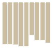
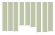

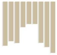
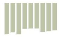

136
6E S 6,12(ii).03 6E S 6,12(ii).02 6E S 6,12(ii).01 6E BS 6,12 (ii) 1 4 7 10 11 12 VOLUME 6E.01(A) 6E.02(A) 6E.03(A) AREA 6E.01(A) 6E.02(A) 6E.03(A) HEIGHT 6E.01(A) 6E.02(A) 6E.03(A) 6F 6,12 (v).03 (C) 6F 6,12 (v).03 (A) 6F 6,12 (v).02 (B) 6F S 6,12 (v).02 (A) 6F 6,12 (v).01 (B) 6F 6,12 (v).01 (A) 6F 6,12 (v).01 (C)6F 6,12 (v).02 (C)6F 6,12 (v).03 (C) VOLUME 6F.02(A) 6F.01(A) 6F.02(B) 6F.01(B) 6F.02(C) 6F.01(C) 6F.03(A) 6F.03(B) 6F.03(C) AREA 6F.02(A) 6F.01(A) 6F.02(B) 6F.01(B) 6F.02(C) 6F.01(C) 6F.03(A) 6F.03(B) 6F.03(C) HEIGHT 6F.02(A) 6F.01(A) 6F.02(B) 6F.01(B) 6F.02(C) 6F.01(C) 6F.03(A) 6F.03(B) 6F.03(C) 6F BS 6,12 (v) 2 4 5 7 9 10 11 12 0 1 6G 6,12(iii). 03 (B) 6G 6,12(iii). 03 (A) 6G 6,12(iii). 02 (B) 6G 6,12(iii). 02 (A) 6G 6,12(iii). 01 (B) 6G 6,12(iii). 01 (A) 6G 6,12(iii). 01 (C) 6G 6,12(iii). 02 (C) 6G 6,12(iii). 03 (C) HEIGHT 6G.02(A) 6G.01(A) 6G.02(B) 6G.01(B) 6G.02(C) 6G.01(C) 6G.03(A) 6G.03(B) 6G.03(C) AREA 6G.02(A) 6G.01(A) 6G.02(B) 6G.01(B) 6G.02(C) 6G.01(C) 6G.03(A) 6G.03(B) 6G.03(C) VOLUME 6G.02(A) 6G.01(A) 6G.02(B) 6G.01(B) 6G.02(C) 6G.01(C) 6G.03(A) 6G.03(B) 6G.03(C) 6G BS 6,12(iii) 4 9 10 11 12 6H S 8,10. 03 (C) 6H S 8,10. 03 (B) 6H 8,10. 03 (A) 6H 8,10. 02 (C) 6H 8,10. 02 (A) 6H 8,10. 01(C) 6H 8,10. 01(B) 6H 8,10. 01(A) 6H 8,10. 02 (B) HEIGHT 6H.02(A) 6H.01(A) 6H.02(B) 6H.01(B) 6H.02(C) 6H.01(C) 6H.03(A) 6H.03(B) 6H.03(C) 6H.02(A) 6H.01(A) 6H.02(B) 6H.01(B) 6H.02(C) 6H.01(C) 6H.03(A) 6H.03(B) 6H.03(C) AREA 6H.02(A) 6H.01(A) 6H.02(B) 6H.01(B) 6H.02(C) 6H.01(C) 6H.03(A) 6H.03(B) 6H.03(C) VOLUME 6H BS 8,10(i) 2 4 9 10 11 12
STRUT
6I 8,10(ii). 01(C)
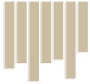
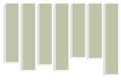

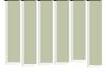
137 6I S 8,10(ii). 02(B0 6I 8,10(ii). 03(A) 6I 8,10(ii). 02(A)
6I 8,10(ii). 02(C) HEIGHT 6I.02(A) 6I.01(A) 6I.02(B) 6I.01(B) 6I.02(C) 6I.01(C) 6I.03(A) 6I.03(B) 6I.03(C) AREA 6I.02(A) 6I.01(A) 6I.02(B) 6I.01(B) 6I.02(C) 6I.01(C) 6I.03(A) 6I.03(B) 6I.03(C) VOLUME 6I.02(A) 6I.01(A) 6I.02(B) 6I.01(B) 6I.02(C) 6I.01(C) 6I.03(A) 6I.03(B) 6I.03(C) 6I BS 8,10(ii) 3 5 6 7 9 10 11 12 HEIGHT 6J.02(A) 6J.01(A) 6J.02(B) 6J.01(B) 6J.03(A) 6J.03(B) AREA 6J.02(A) 6J.01(A) 6J.02(B) 6J.01(B) 6J.03(A) 6J.03(B) VOLUME 6J.02(A) 6J.01(A) 6J.02(B) 6J.01(B) 6J.03(A) 6J.03(B) 6J 8,10(iii). 03(B) 6J 8,10(iii). 03(A) 6J 8,10(iii). 02(A) 6J 8,10(iii). 01(A) 2 6 7 8 9 10 11 12 6J BS 8,10(iii) 6J 8,10(iii). 01(B) 6J 8,10(iii). 02(B)
6I 8,10(ii). 01(B) 6I 8,10(ii). 01(A)
MORPHOLOGY GENERATION - 7 STRUT
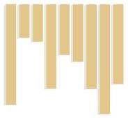


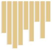
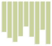

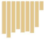
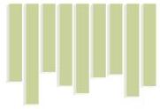


138
7A.01(A) 7A.02(A) 7A.01(B) 7A.02(B) 7A.01(C) 7A.02(C) 7A.03(A) 7A.03(B) 7A.03(C) 7A.01(A) 7A.02(A) 7A.01(B) 7A.02(B) 7A.01(C) 7A.02(C) 7A.03(A) 7A.03(B) 7A.03(C) VOLUME 7A.01(A) 7A.02(A) 7A.01(B) 7A.02(B) 7A.01(C) 7A.02(C) 7A.03(A) 7A.03(B) 7A.03(C) HEIGHT AREA 7A S 6,15(i).03 (C) 7A S 6,15(i).03 (B) 7A S 6,15(i).03 (A) 7A S 6,15(i).02 (C) 7A S 6,15(i).02 (B) 7A S 6,15(i).02 (A) 7A 6,15(i). 01(C) 7A S 6,15(i). 01(B) 7A 6,15(i). 01(A) 7A BS 6,15(i) 4 6 10 11 12 13 14 VOLUME 7B.01(A) 7B.02(A) 7B.01(B) 7B.02(B) 7B.03(A) 7B.03(B) 7B.01(C) 7B.02(C) 7B.03(C) AREA 7B.01(A) 7B.02(A) 7B.01(B) 7B.02(B) 7B.03(A) 7B.03(B) 7B.01(C) 7B.02(C) 7B.03(C) HEIGHT 7B.01(A) 7B.02(A) 7B.01(B) 7B.02(B) 7B.03(A) 7B.03(B) 7B.01(C) 7B.02(C) 7B.03(C) 7B S 6,15(ii). 03(C) 7B S 6,15(ii). 03(B) 7B S 6,15(ii). 03(A) 7B S 6,15(ii). 02(C) 7B S 6,15(ii). 02(B) 7B S 6,15(ii). 02(A) 7B S 6,15(ii). 01(C) 7B S 6,15(ii). 01(B) 7B S 6,15(ii). 01(A) 7B BS 6,15(ii) 2 4 5 6 8 10 11 12 13 14 5(ii) VOLUME 7C.02(A) 7C.01(A) 7C.02(C) 7C.01(C) 7C.03(A) 7C.02(B) 7C.01(B) 7C.03(B) 7C.03(C) AREA 7C.02(A) 7C.01(A) 7C.02(C) 7C.01(C) 7C.03(A) 7C.02(B) 7C.01(B) 7C.03(B) 7C.03(C) HEIGHT 7C.02(A) 7C.01(A) 7C.02(C) 7C.01(C) 7C.03(A) 7C.02(B) 7C.01(B) 7C.03(B) 7C.03(C) 7C S 8,13(i).03 (C) 7C S 8,13(i).03 (B) 7C S 8,13(i).03 (A) 7C S 8,13(i).02 (C) 7C S 8,13(i).02 (B) 7C S 8,13(i).02 (A) 7C S 8,13(i).01(C) 7C 8,13(i).01(B) 7C S 8,13(i).01(A) 7C BS 8,13(i) 3 7 8 9 10 11 12 13 14 7D S 10,11(i). 02(A) 7D S 10,11(i). 01(C) 7D 10,11(i). 01(B) 7D S 10,11(i). 01(A) VOLUME 7D.02(A) 7D.01(A) 7D.01(B) 7D.01(C) AREA 7D.02(A) 7D.01(A) 7D.01(B) 7D.01(C) HEIGHT 7D.02(A) 7D.01(A) 7D.01(B) 7D.01(C) 7D BS 10,11(i) 1 2 4 5 8 9 10 11 12 13 14 1 1
7E S 10,11(ii). 01(A)


S 10,11(ii). 02(A)
S 10,11(ii). 03(B) 7E S 10,11(ii). 03(A)
7E S 10,11(ii). 01(B)
7E S 10,11(ii). 01(C)
S 10,11(ii). 03(C)

139
7E
7E
7E
7E.02(A) 7E.01(A) 7E.01(B) 7E.01(C) 7E.03(A) 7E.03(B) 7E.03(C) VOLUME 7E.02(A) 7E.01(A) 7E.01(B) 7E.01(C) 7E.03(A) 7E.03(B) 7E.03(C) AREA HEIGHT 7E.02(A) 7E.01(A) 7E.01(B) 7E.01(C) 7E.03(A) 7E.03(B) 7E.03(C) 7E BS 10,11(ii) 1 4 5 6 9 10 11 12 13 14 7F.02(A) 7F.01(A) 7F.02(B) 7F.01(B) 7F.02(C) 7F.01(C) 7F.03(A) 7F.03(B) 7F.03(C) VOLUME 7F.02(A) 7F.01(A) 7F.02(B) 7F.01(B) 7F.02(C) 7F.01(C) 7F.03(A) 7F.03(B) 7F.03(C) HEIGHT 7F.02(A) 7F.01(A) 7F.02(B) 7F.01(B) 7F.02(C) 7F.01(C) 7F.03(A) 7F.03(B) 7F.03(C) AREA 7F 6,15(iii). 03(A)
S 6,15(iii). 02(B) 7F S 6,15(iii). 03(C) 7F S 6,15(iii). 03(B) 7F S 6,15(iii). 02(C) 7F S 6,15(iii). 02(A)
7F
7F
7F
1 2 4 6 7
7G
7G
7G
7G S 6,15(iv). 02(A) 7G S 6,15(iv). 01(C) 7G S 6,15(iv). 01(B) 7G S 6,15(iv). 01(A) 7G.02(A) 7G.01(A) 7G.02(B) 7G.01(B) 7G.02(C) 7G.01(C) 7G.03(A) 7G.03(B) 7G.03(C) VOLUME 7G.02(A) 7G.01(A) 7G.02(B) 7G.01(B) 7G.02(C) 7G.01(C) 7G.03(A) 7G.03(B) 7G.03(C) AREA 7G.02(A) 7G.01(A) 7G.02(B) 7G.01(B) 7G.02(C) 7G.01(C) 7G.03(A) 7G.03(B) 7G.03(C) HEIGHT 7G BS 6,15(iv) 2 3 5 8 10 11 12 13 14 7H BS 8,13(ii) 2 5 10 11 12 13 14
7F S 6,15(iii). 01(C)
6,15(iii). 01(B)
6,15(iii). 01(A) 7F BS 6,15(iii)
8 9 10 11 12 13 14 3 7G S 6,15(iv). 02(B)
S 6,15(iv). 03(C)
S 6,15(iv). 03(B)
S 6,15(iv). 03(A) 7G S 6,15(iv). 02(C)


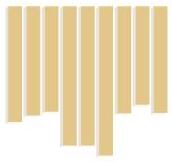
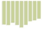

140 VOLUME 7J.02(A) 7J.01(A) 7J.02(B) 7J.01(B) 7J.02(C) 7J.01(C) 7J.03(A) 7J.03(B) 7J.03(C) AREA 7J.02(A) 7J.01(A) 7J.02(B) 7J.01(B) 7J.02(C) 7J.01(C) 7J.03(A) 7J.03(B) 7J.03(C) HEIGHT 7J.02(A) 7J.01(A) 7J.02(B) 7J.01(B) 7J.02(C) 7J.01(C) 7J.03(A) 7J.03(B) 7J.03(C) 7I.02(A) 7I.01(A) 7I.02(B) 7I.01(B) 7I.02(C) 7I.01(C) 7I.03(A) 7I.03(B) 7I.03(C) VOLUME 7I.02(A) 7I.01(A) 7I.02(B) 7I.01(B) 7I.02(C) 7I.01(C) 7I.03(A) 7I.03(B) 7I.03(C) AREA HEIGHT 7I.02(A) 7I.01(A) 7I.02(B) 7I.01(B) 7I.02(C) 7I.01(C) 7I.03(A) 7I.03(B) 7I.03(C) 7I
01(A) 7I S 6,15(v). 03(C) 7I 6,15(v). 03(B) 7I 6,15(v). 03(A) 7I S 6,15(v). 02(C) 7I 6,15(v). 02(B) 7I 6,15(v). 02(A)
S 6,15(v). 01(C) 7I S 6,15(v). 01(B) 7I BS 6,15(v) 3 6 7 8 9 10 11 12 13 14 4 7J S 10,11(iii). 03(C) 7J S 10,11(iii). 03(B) 7J S 10,11(iii). 03(A) 7J 10,11(iii). 02(C) 7J S 10,11(iii). 02(B) 7J
01(C) 7J
01(B) 7J
01(A) 7J S 10,11(iii). 02(A)
BS 10,11(iii)
2 3 5 6 10 11 12 13 14 1(iii) 1
S 6,15(v).
7I
S 10,11(iii).
S 10,11(iii).
S 10,11(iii).
7J
1
MORPHOLOGY
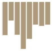


S10,14(i).02(A)
8C S10,14(i).02(C) 8C S10,14(i).02(B)
S10,14(i).05(A)
8C S10,14(i).04(C) 8C S10,14(i).04(B) 8C S10,14(i).04(A) 8C
8B BS8,16(i) 1 4 6 10 11 12 13 14 15 16
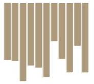
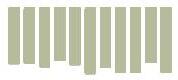

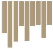
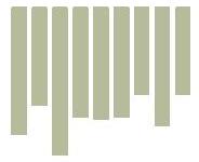

8B S8,16(i).05(A)
8BS8,16(i).01(A)
8B S8,16(i).02(A)
8B S8,16(i).02(B)
8B S8,16(i).04(B)
8B S8,16(i).05(B)
8B S8,16(i).01(B)
8B S8,16(i).01(C)
8B S8,16(i).02(C)
8B S8,16(i).04(C)
8B S8,16(i).05(C)
8D
8D S12,12(ii).05(B)
141
8 STRUT 9A.01(A) 9A.01(B) 9A.02(B) 9A.01(C) 9A.02(C) 9A.03(A) 9A.05(A) 9A.05(C) VOLUME 9A.01(A) 9A.01(B) 9A.02(B) 9A.01(C) 9A.02(C) 9A.03(A) 9A.05(A) 9A.05(C) AREA 9A.01(A) 9A.01(B) 9A.02(B) 9A.01(C) 9A.02(C) 9A.03(A) 9A.05(A) 9A.05(C) HEIGHT 8A S12,12(i).05(C) 8A S12,12(i).05(A) 8A S12,12(i).03(A) 8A S12,12(i).02(C) 8A S12,12(i).02(B) 8A S12,12(i).01(C) 8A S12,12(i).01(B) 8A S12,12(i).01(A) 8A BS12,12(i) 4 8 10 11 12 13 14 15 16 1 9B.01(A) 9B.02(A) 9B.01(B) 9B.02(B) 9B.01(C) 9B.02(C) 9B.04(B) 9B.04(C) 9B.05(A) 9B.05(B) 9B.05(C) VOLUME 9B.01(A) 9B.02(A) 9B.01(B) 9B.02(B) 9B.01(C) 9B.02(C) 9B.04(B) 9B.04(C) 9B.05(A) 9B.05(B) 9B.05(C) HEIGHT 9B.01(A) 9B.02(A) 9B.01(B) 9B.02(B) 9B.01(C) 9B.02(C) 9B.04(B) 9B.04(C) 9B.05(A) 9B.05(B) 9B.05(C) AREA
GENERATION -
9C.02(A) 9C.01(A) 9C.02(C) 9C.01(C) 9C.03(A) 9C.02(B) 9C.01(B) 9C.03(B) 9C.04(C) 9C.04(A) 9C.04(B) 9C.05(A) AREA
8C
8C
S10,14(i).03(B)
S10,14(i).03(A)
8C
8C S10,14(i).01(B) 9C.02(A) 9C.01(A) 9C.02(C) 9C.01(C) 9C.03(A) 9C.02(B) 9C.01(B) 9C.03(B) 9C.04(C) 9C.04(A) 9C.04(B) 9C.05(A) VOLUME 9C.02(A) 9C.01(A) 9C.02(C) 9C.01(C) 9C.03(A) 9C.02(B) 9C.01(B) 9C.03(B) 9C.04(C) 9C.04(A) 9C.04(B) 9C.05(A) HEIGHT 8C BS10,14(i) 1 2 3 4 10 11 12 13 14 15 16 1
8C
8C S10,14(i).01(C)
S10,14(i).01(A)
S12,12(ii).04(C) 8D S12,12(ii).03(B) 8D S12,12(ii).03(A) 8D S12,12(ii).02(C) 8D
8D S12,12(ii).01(C) 8D S12,12(ii).01(B) 8D S12,12(ii).01(A) 9D.02(A) 9D.01(A) 9D.01(B) 9D.02(C) 9D.01(C) 9D.03(A) 9D.03(B) 9D.04(C) 9D.05(B) VOLUME 9D.02(A) 9D.01(A) 9D.01(B) 9D.02(C) 9D.01(C) 9D.03(A) 9D.03(B) 9D.04(C) 9D.05(B) AREA 9D.02(A) 9D.01(A) 9D.01(B) 9D.02(C) 9D.01(C) 9D.03(A) 9D.03(B) 9D.04(C) 9D.05(B) HEIGHT 1 2 10 11 12 13 14 15 16 8D BS12,12(ii)
S12,12(ii).02(A)
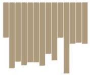

BS6,18(i)
8E S6,18(i).02(A)
8E S6,18(i).01(A)
8E S6,18(i).01(B)
8E S6,18(i).01(C)
S6,18(i).03(B) 8E S6,18(i).02(C) 8E S6,18(i).02(B)
S6,18(i).04(A) 8E S6,18(i).03(C)
S6,18(i).04(B)
S6,18(i).05(A) 8E S6,18(i).04(C)
S6,18(i).05(B)
S6,18(i).05(C)
142 9E.02(A) 9E.01(A) 9E.02(B) 9E.01(B) 9E.02(C) 9E.01(C) 9E.03(B) 9E.03(C) 9E.04(A) 9E.04(B) 9E.04(C) 9E.05(A) 9E.05(B) 9E.05(C) VOLUME 9E.02(A) 9E.01(A) 9E.02(B) 9E.01(B) 9E.02(C) 9E.01(C) 9E.03(B) 9E.03(C) 9E.04(A) 9E.04(B) 9E.04(C) 9E.05(A) 9E.05(B) 9E.05(C) AREA 9E.02(A) 9E.01(A) 9E.02(B) 9E.01(B) 9E.02(C) 9E.01(C) 9E.03(B) 9E.03(C) 9E.04(A) 9E.04(B) 9E.04(C) 9E.05(A) 9E.05(B) 9E.05(C) HEIGHT 8E
8E
8E
8E
8E
8E
1 3 8 9 10 11 12 13 14 15 16 8E
1 1
S 12,15(i). 01(A) 9B S 12,15(i). 01(B)


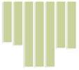
9B S 12,15(i). 02(A)

S 12,15(i). 02(B)
143
STRUT VOLUME 9A.01(A) 9A.02(A) 9A.01(B) 9A.02(B) 9A.01(C) 9A.02(C) 9A.03(A) 9A.03(B) AREA 9A.01(A) 9A.02(A) 9A.01(B) 9A.02(B) 9A.01(C) 9A.02(C) 9A.03(A) 9A.03(B) HEIGHT 9A.01(A) 9A.02(A) 9A.01(B) 9A.02(B) 9A.01(C) 9A.02(C) 9A.03(A) 9A.03(B) 9A S 14,13(i).03(A) 9A 14,13(i).02(B) 9A S 14,13(i).02(A) 9A S 14,13(i).01(B) 9A S 14,13(i).01(A) 9A S 14,13(i).01(C) 9A S 14,13(i).03(B) 9A S 14,13(i).02(C) 9A BS 14,13(i) 1 4 10 11 12 13 14 15 16 17 18 9B.01(A) 9B.02(A) 9B.01(B) 9B.02(B) 9B.03(A) 9B.03(B) 9B.02(C) HEIGHT
9B S 12,15(i). 02(C) 9B S 12,15(i). 03(A) 9B S 12,15(i). 03(B) 9B BS 12,15(i) 1 5 8 10 11 12 13 14 15 16 17 18 1 VOLUME 9B.01(A) 9B.02(A) 9B.01(B) 9B.02(B) 9B.03(A) 9B.03(B) 9B.02(C)
9B.01(A) 9B.02(A) 9B.01(B) 9B.02(B) 9B.03(A) 9B.03(B) 9B.02(C) 9C
03(A) 9C
02(A)
S 16,11(i). 01(A) 9C.02(A) 9C.01(A) 9C.01(C) 9C.03(A) 9C.01(B) VOLUME 9C.02(A) 9C.01(A) 9C.01(C) 9C.03(A) 9C.01(B) AREA 9C.02(A) 9C.01(A) 9C.01(C) 9C.03(A) 9C.01(B) A) A) HEIGHT
1 4 5
10 11 12 13 14 15 16 17 18 1 9D BS 12,15(ii) 5 7 10 11 12 13 14 15 16 17 18
MORPHOLOGY GENERATION - 9
9B
9B
) ) ) AREA
S 16,11(i).
S 16,11(i).
9C S 16,11(i). 01(C) 9C S 16,11(i). 01(B) 9C
9C BS 16,11(i)
8
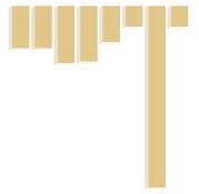
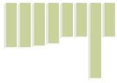

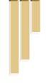


144 3 5 6 10 11 12 13 14 15 16 17 18 9G BS14,13(iii) 1 VOLUME 9H.02(A) 9H.01(A) 9H.02(B) AREA 9H.02(A) 9H.01(A) 9H.02(B) HEIGHT 9H.02(A) 9H.01(A) 9H.02(B) 9H S12,15(iv).02(B) 9H S12,15(iv).02(A) 9H S12,15(iv).01(A) 9H BS12,15(iv) 1 4 9 10 11 12 13 14 15 16 17 18 9F S14,13(ii).02(A)
9F
9F S14,13(ii).02(B) 9F S14,13(ii).02(C) VOLUME 9F.02(A) 9F.01(A) 9F.02(B) 9F.01(B) 9F.02(C) 9F.01(C) AREA 9F.02(A) 9F.01(A) 9F.02(B) 9F.01(B) 9F.02(C) 9F.01(C) HEIGHT 9F.02(A) 9F.01(A) 9F.02(B) 9F.01(B) 9F.02(C) 9F.01(C) 9F BS14,13(ii) 2 3 4 8 10 11 12 13 14 15 16 17 18 VOLUME 9E.02(A) 9E.01(A) 9E.02(B) 9E.01(B) 9E.02(C) 9E.01(C) 9E.03(A) 9E.03(B) AREA 9E.02(A) 9E.01(A) 9E.02(B) 9E.01(B) 9E.02(C) 9E.01(C) 9E.03(A) 9E.03(B) HEIGHT 9E.02(A) 9E.01(A) 9E.02(B) 9E.01(B) 9E.02(C) 9E.01(C) 9E.03(A) 9E.03(B) 9E S 12,15(iii). 03(A) 9E S 12,15(iii). 02(C) 9E S 12,15(iii). 02(B) 9E 12,15(iii). 02(A) 9E S 12,15(iii). 01(B) 9E S 12,15(iii). 01(A) 9E S 12,15(iii). 03(B) 9E S 12,15(iii). 01(C)
BS 12,15(iii) 2 4 7 9 10 11 12 13 14 15 16 17 18
9F S14,13(ii).01(C) 9F S14,13(ii).01(B)
S14,13(ii).01(A)
9E
9J S14,13(iv).01(A)


9J S14,13(iv).01(C)


145
VOLUME 9J.01(A) 9J.01(C) AREA 9J.01(A) 9J.01(C) HEIGHT 9J.01(A) 9J.01(C)
BS14,13(iv) 1 2 3 6 7 8 10 11 12 13 14 15 16 17 18 1 VOLUME 9I.01(A) 9I.01(B) 9I.02(C) 9I.01(C) AREA 9I.01(A) 9I.01(B) 9I.02(C) 9I.01(C) HEIGHT 9I.01(A) 9I.01(B) 9I.02(C) 9I.01(C)
BS12,15(v) 1 3 4 9 10 11 12 13 14 15 16 17 18 1
9J
9I S12,15(v).02(C) 9I S12,15(v).01(C) 9I S12,15(v).01(B) 9I S12,15(v).01(A) 9I
EVALUATION STAGE 2
146
0 1000 2000 3000 4000 5000 6000 7000 S:5S:1S:6S:2S:3S:4 0 1000 2000 3000 4000 5000 6000 7000 STRUT LENGTH STRUT LENGTH CABLE LENGTH S3 S4 S1 S6 S2 EC EC 7 EC 2 EC 6 EC 5 EC 8 EC 12 EC 11 EC 9 EC 1 NEC 5 NEC NEC 2 NEC 4 NEC 1 NEC 3 X Y Y 0 1000 2000 3000 4000 5000 S:3S:6S:1S:2S:5S:4 6000 7000 0 1000 2000 3000 4000 5000 6000 7000 STRUT LENGTH STRUT LENGTH CABLE LENGTH S2 S6 S4 S5 S1 S3 EC 1 EC 6 EC 3 EC 12 EC 5 EC 2 EC 8 EC 4 EC 10 NEC 5 NEC 1 NEC 3 NEC 4 NEC 6 X Z Z Y Y Y STRUT LENGTH STRUT LENGTH CABLE LENGTH NEC Y Y NEC 2 NEC 3 S2 S3 S5 S4 S1 EC 6 EC 9 EC 8 EC 10 EC 2 EC 5 EC 7 EC 11 NEC 1 0 1000 2000 3000 4000 5000 6000 7000 EC:4 EC:3 EC:11 EC:9 EC:2 EC:10 NEC:3 EC:1 EC:7 EC:5 EC:6 EC:8 NEC:1 NEC:2 NEC:4 0 1000 2000 3000 4000 5000 6000 7000 S 5 S 1 S 3 S 2 S:4 N S S E C C 1 C N 0 1000 2000 3000 4000 5000 6000 S:5S:4S:1S:2S:3 7000 0 1000 2000 3000 4000 5000 6000 7000 EC:6 EC:5 EC:7 EC:4 EC:3 EC:2 EC:1 NEC:1 NEC:6 NEC:4 NEC:5 NEC:8 NEC:3 NEC:7 NEC:2 STRUT LENGTH STRUT LENGTH CABLE LENGTH S3 S1 S5 S2 S4 EC EC 1 EC 1 EC 7 EC 5 EC 6 NEC 7 NEC 8 NEC 4 NEC 3 NEC 1 NEC 2 NEC 5 X Y Y Z X Y Y Y Y S S S E E 5 0 1000 2000 3000 4000 5000 6000 7000
0 1000 2000 3000 4000 5000 6000 7000 STRUT LENGTH STRUT LENGTH CABLE LENGTH S3 S1 S4 S2 S5 S6 EC 1 EC 8 EC 7 EC 6 EC 4 EC 5 EC 2 EC 3 NEC 2 NEC 9 NEC 8 NEC 4 NEC NEC 1 NEC 10 NEC 7 NEC 6 X Z Y Y S 5 6 C N
S:6S:2S:5S:3S:1S:4
S:2S:1S:6S:5S:3S:4
S:6S:5S:1S:7S:3S:2S:4
147 0 1000 2000 3000 4000 5000 6000 7000 S:1S:2S:5S:6S:4S:3 0 1000 2000 3000 4000 5000 6000 7000 STRUT LENGTH STRUT LENGTH CABLE LENGTH INTERSECTION POINTS = 2 S2 S3 S5 S6 S1 S4 EC 1 EC 3 EC 4 EC 2 EC EC 9 EC 10 EC 8 NEC 5 NEC NEC 7 NEC 2 NEC 4 NEC 3 NEC 8 NEC 1 Z 0 1000 2000 3000 4000 5000 6000 7000 S:3S:4S:7S:2S:1S:5S:6 0 1000 2000 3000 4000 5000 6000 7000 STRUT LENGTH STRUT LENGTH CABLE LENGTH INTERSECTION POINTS = 1 S2 S3 S7 S5 S6 S1 S4 EC 3 EC 1 EC EC 5 EC 6 EC 10 EC 13 EC 12 EC 11 EC 8 X X Z Y 0 1000 2000 3000 4000 5000 6000 7000
0 1000 2000 3000 4000 5000 6000 7000 STRUT LENGTH STRUT LENGTH CABLE LENGTH S3 S5 S6 S4 S1 S7 S2 EC EC 9 EC 5 EC 7 EC 11 EC 10 EC 4 EC EC 3 EC 8 NEC 6 NEC 2 NEC 9 NEC 7 NEC 4 NEC NEC 10 Z Z Y Y 0 1000 2000 3000 4000 5000 6000 7000
S:7S:1S:5S:6S:3S:2S:4
0 1000 2000 3000 4000 5000 6000 7000 STRUT LENGTH STRUT LENGTH CABLE LENGTH S2 S2 S7 S4 S3 S1 S6 EC EC 8 EC EC EC EC 4 EC 9 EC EC 11 NEC 6 NEC NEC 10 NEC NEC 1 NEC 7 NEC NEC 4 X X Y 4 1 EC3 E C N C5 N S3 S2 S6 S5 S4 EC 5 EC EC 11 EC 12 EC EC 10 EC EC 2 EC EC EC NEC NEC NEC NEC NEC NEC 0 1000 2000 3000 4000 5000 6000 7000
0 1000 2000 3000 4000 5000 6000 7000 STRUT LENGTH STRUT LENGTH CABLE LENGTH INTERSECTION POINTS =
S:8S:3S:7S:5S:1S:2S:4S:6
148 0 1000 2000 3000 4000 5000 6000 7000 S:7S:6S:5S:1S:4S:2S:3 0 1000 2000 3000 4000 5000 6000 7000 STRUT LENGTH STRUT LENGTH CABLE LENGTH INTERSECTION POINTS = S6 S1 S4 S3 S2 S7 S5 EC 2 EC 9 EC 7 EC 12 EC 15EC 10 EC 3 EC 13 EC EC 5 EC 14 NEC 6 NEC 5 NEC NEC 4 NEC 1 NEC 0 1000 2000 3000 4000 5000 6000 S:1S:6S:2S:7S:8S:3S:4S:5 7000 0 1000 2000 3000 4000 5000 6000 7000 STRUT LENGTH STRUT LENGTH CABLE LENGTH INTERSECTION POINTS = S6 S1 S4 S3 S8 S2 S7 S5 EC EC EC 7 EC 12 EC 11 EC 10 EC 3 EC 2 EC 5 NEC 6 NEC 5 NEC 2 NEC 4 NEC 7 NEC 11 NEC 10 NEC 9 NEC 8 NEC 1 NEC NEC 12 X X X Z Y 0 1000 2000 3000 4000 5000 6000 7000 S:8S:3S:7S:1S:2S:6S:4S:5 0 1000 2000 3000 4000 5000 6000 7000 STRUT LENGTH STRUT LENGTH CABLE LENGTH INTERSECTION POINTS = S6 S1 S4 S3 S2 S7 S5 S8 EC 2 EC 9 EC 7 EC 12 EC 1 EC 3 EC 6 EC 11 EC 8 NEC NEC 7 NEC 11 NEC NEC 5 NEC 2 NEC 4 NEC 1 NEC 10 NEC 3 Z Z 0 1000 2000 3000 4000 5000 6000 7000
0 1000 2000 3000 4000 5000 6000 7000 STRUT LENGTH STRUT LENGTH CABLE LENGTH S6 S1 S4 S3 S2 S7 S8 S5 EC 2 EC 7 EC 10 EC 3 EC 13 EC 6 EC 8 EC 5 NEC 6 NEC 10 NEC NEC 2 NEC 4 NEC 1 NEC 8 NEC 7 NEC X X Z Y Y Y 0 1000 2000 3000 4000 5000 6000
7000 0 1000 2000 3000 4000 5000 6000 7000 STRUT LENGTH STRUT LENGTH CABLE LENGTH S3 S4 S6 S7 S5 S1 S2 EC 3 EC 15 EC 1 EC EC 12 EC 6 EC 8 EC EC 10 EC 2 EC 11 EC 13 EC 7 NEC NEC 4 NEC 2 NEC 3 NEC 5 Z Y S C3 E E C C 0 3 C N N
S:5S:7S:4S:6S:3S:1S:2
S:7S:4S:9S:2S:5S:8S:1S:3S:6
S:6S:3S:5S:1S:8S:2S:9S:7S:4
S:3S:6S:4S:5S:9S:7S:8S:1S:2
149 0 1000 2000 3000 4000 5000 6000 7000
0 1000 2000 3000 4000 5000 6000 7000 NEC:2 EC:7 NEC:7 EC:13 EC:5 NEC:5 NEC:6 EC:15 EC:14 NEC:3 NEC:11 NEC:1 EC:6 EC:10 STRUT LENGTH STRUT LENGTH CABLE LENGTH S6 S1 S3 S2 S8 S5 EC 2 EC 9 EC 9 EC 12 EC 11 EC 15 EC 10 EC 4 EC 13 EC 6 EC 5 NEC 5 NEC 7 NEC 10 NEC 9 NEC 12 NEC 11 NEC 4 NEC 1 NEC 3 X Z 0 1000 2000 3000 4000 5000 6000 7000
0 1000 2000 3000 4000 5000 6000 7000 NEC:11 EC:1 EC:7 EC:13 NEC:6 EC:9 NEC:4 NEC:8 EC:10 EC:5 EC:6 NEC:1 NEC:12 NEC:5 STRUT LENGTH STRUT LENGTH CABLE LENGTH INTERSECTION POINTS 2 S1 S4 S8 S3 S2 S7 S9 S5 EC 2 EC 9 EC 12 EC 15 EC 10 EC EC EC 6 EC EC 14 NEC 6 NEC NEC 9 NEC 8 NEC 2 NEC 7 NEC 10 NEC 4 NEC NEC 12 X Z Z Y 0 1000 2000 3000 4000 5000 6000 7000
0 1000 2000 3000 4000 5000 EC:6 EC:2 EC:14 EC:9 NEC:5 EC:1 EC:11 NEC:9 NEC:1 EC:8 NEC:3 NEC:6 NEC:7 NEC:11 6000 7000 STRUT LENGTH STRUT LENGTH CABLE LENGTH INTERSECTION POINTS 4 S6 S9 S1 S4 S3 S2 S7 EC 1 EC 12 EC 3 EC 4 EC 11 NEC NEC 7 NEC 5 NEC 2 NEC 10 NEC 1 NEC 3 NEC 11 X Y Y 0 1000 2000 3000 4000 5000 6000 7000 S:7S:8S:9S:1S:2S:6S:4 S:3 S:5 0 1000 2000 3000 4000 5000 6000 7000 NEC:2 EC:10 EC:6 EC:1 EC:3 NEC:6 EC:2 EC:11 NEC:4 NEC:10 NEC:12 NEC:5 NEC:9 NEC:14 STRUT LENGTH STRUT LENGTH CABLE LENGTH S6 S1 S9 S4 S3 S2 S7 S5 EC 2 EC EC 7 EC 12 EC 6 EC EC EC 4 NEC 6 NEC 8 NEC 9 NEC 5 NEC 13 NEC 14 NEC 4 NEC 1 NEC 10 NEC 11 NEC 12 X Z INTERSECTION POINTS =
Linear Static Analysis Test on selected module.
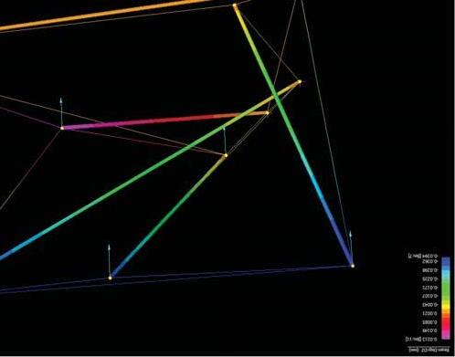

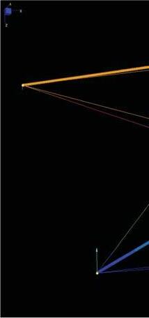
Failed Structure using Linear Buckling Analysis Test on selected module under design loads
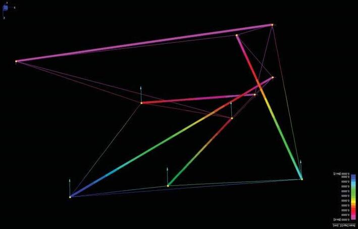
Stable Structure using Linear Buckling Analysis Test on selected module under design loads
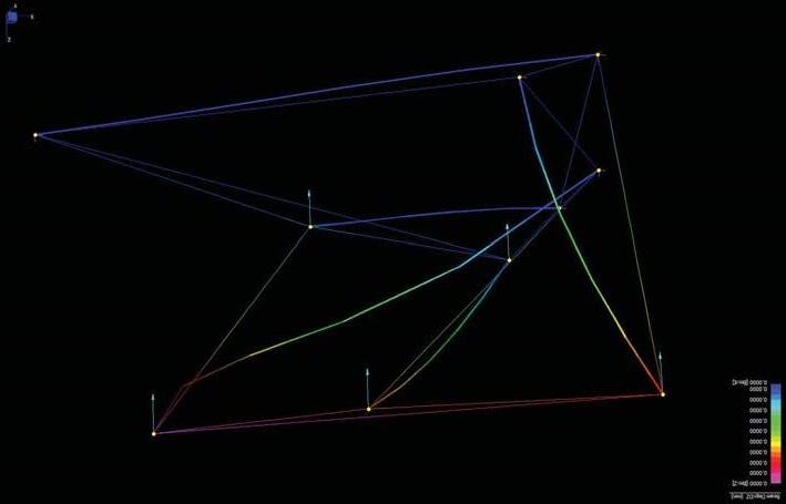
150
ANALYSIS
STRAND
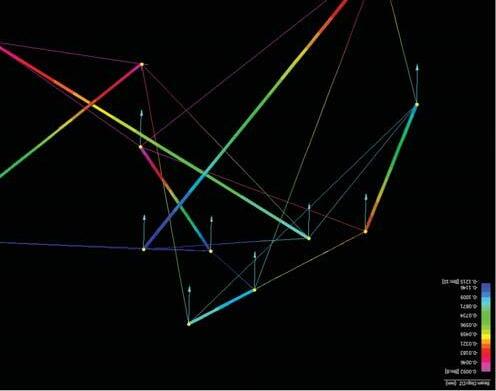

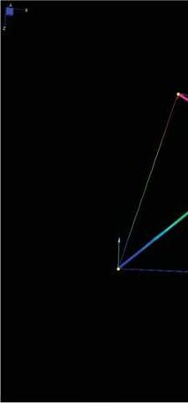
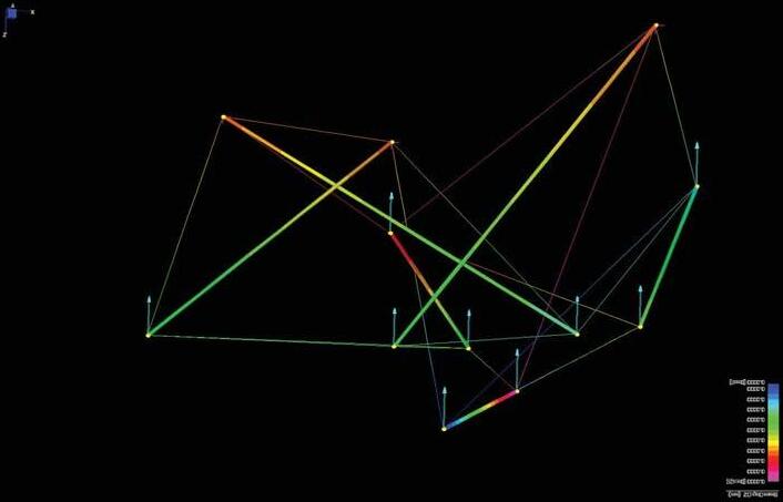
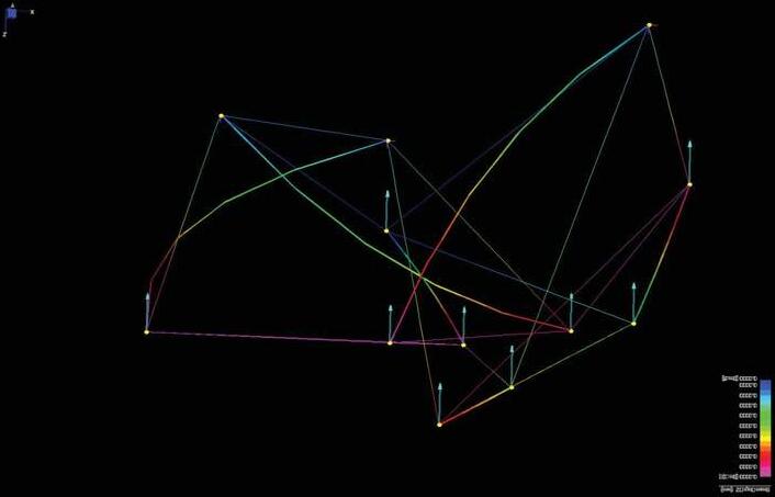
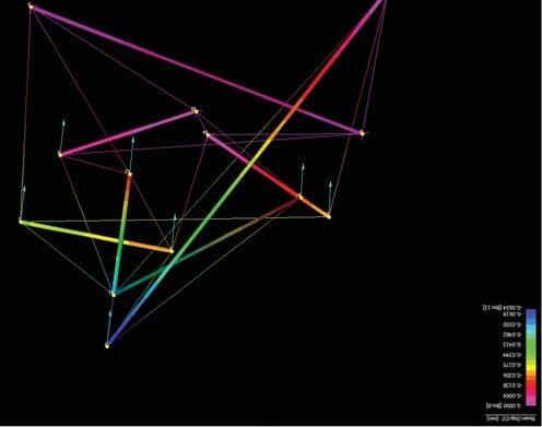


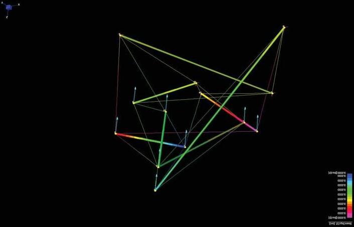
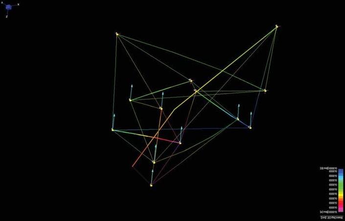
151
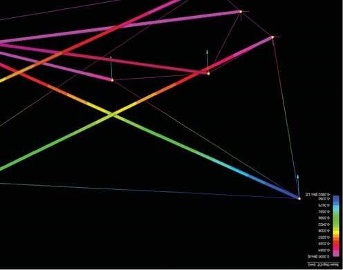

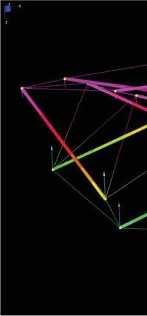
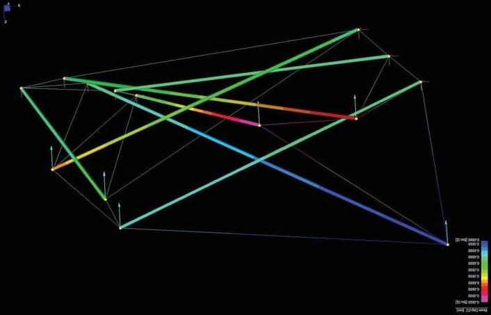
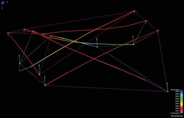
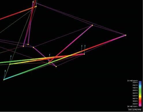

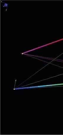
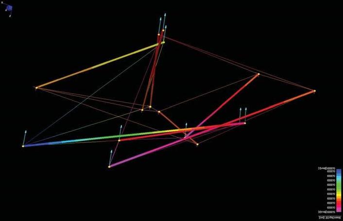
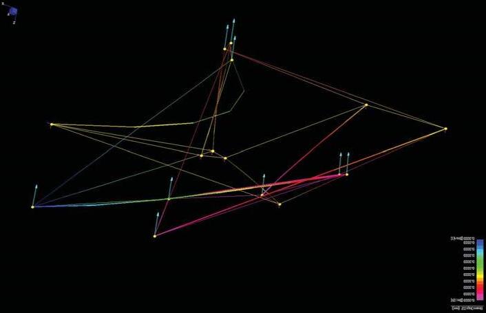
152

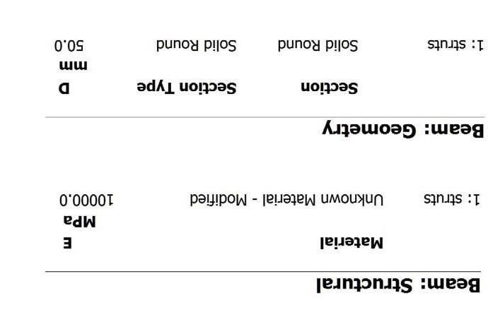
153
MODULE ORIENTATION CATALOGUE
154
5A S4,11. 01 (1-5-7-8) 1 2 3 5 6 7 8 9 10 1 3 6 7 8 9 10 5A S4,11. 01 (1-8-10) 1 2 3 5 6 7 8 9 10 1 3 5 6 7 8 9 10 12 3 5 6 7 8 9 10 5A S4,11. 01 (2-4-8) 1 2 3 5 6 7 8 9 10 1 2 3 5 6 7 8 9 10 1 2 3 5 6 8 9 10 5A S4,11. 01 (3-5-7) 12 3 5 6 7 8 9 10 5A S4,11. 01 (4-8-10) 1 2 3 5 6 7 8 9 10 1 2 3 5 6 7 8 9 10 1 2 3 5 6 7 8 9 10 1 2 3 5 6 7 8 9 10 4 1 2 3 4 5 6 7 8 9 10 1 2 3 4 5 6 7 8 9 10 PLAN VIEW FRONT ELEVATIONSIDE ELEVATION PLAN VIEW FRONT ELEVATIONSIDE ELEVATION PLAN VIEW FRONT ELEVATIONSIDE ELEVATION PLAN VIEW FRONT ELEVATIONSIDE ELEVATION PLAN VIEW FRONT ELEVATIONSIDE ELEVATION
155 5C S8,7 .02(A) (1-2-6) 5C S8,7 .02(A) (1-5-7) 5C S8,7 .02(A) (1-6-8) 5C S8,7 .02(A) (2-6-7) 5C S8,7 .02(A) (6-7-8) 1 2 3 4 5 6 7 8 9 10 1 2 3 4 5 6 7 8 9 10 1 2 3 4 5 6 7 8 9 10 1 2 3 4 5 6 7 8 9 10 1 2 3 4 5 6 7 8 9 10 1 2 3 4 5 6 7 8 9 10 1 2 3 4 5 6 7 8 9 10 1 2 3 4 5 6 7 8 9 10 1 2 3 4 5 6 7 8 9 10 1 2 3 4 5 6 7 8 9 10 1 2 3 4 5 6 7 8 9 10 1 2 3 4 5 6 7 8 9 10 1 2 3 4 5 67 8 9 10 1 2 3 4 5 6 8 9 10 7 1 2 3 4 5 68 9 10 PLAN VIEW FRONT ELEVATIONSIDE ELEVATION PLAN VIEW FRONT ELEVATIONSIDE ELEVATION PLAN VIEW FRONT ELEVATIONSIDE ELEVATION PLAN VIEW FRONT ELEVATIONSIDE ELEVATION PLAN VIEW FRONT ELEVATIONSIDE ELEVATION Base Area = 9.25 SqMts Base Area = 7.00 SqMts Base Area = 4.34 SqMts Base Area = 9.83 SqMts Base Area = 7.12 SqMts Clear Ht Max Ht Clear Ht Max Ht Clear Ht Max Ht Clear Ht Max Ht Clear Ht Max Ht 1.8 M 1.8 M 1.8 M 1.8 M 1.8 M

156 6A
10,8(i). 01(A)
6A
10,8(i). 01(A)
6A
10,8(i). 01(A)
6A S 10,8(i). 01(A) (2-6-8-9) 6A S 10,8(i). 01(A) (2-8-9-10) 1 2 3 4 5 6 7 8 9 10 11 12 1 2 3 4 5 6 7 8 9 10 11 12 1 2 3 4 5 6 7 8 9 10 11 12 1 2 3 4 5 6 7 8 9 10 11 12 1 2 3 4 5 6 7 8 9 10 11 12 1 2 3 4 5 6 7 8 9 10 11 12 1 2 3 4 5 6 7 8 9 10 11 12 1 2 3 4 5 6 7 8 9 10 11 12 1 2 3 4 5 6 7 8 9 10 11 12 1 2 3 4 5 6 7 8 9 10 11 12 1 2 3 4 5 6 7 8 9 10 11 12 1 2 3 4 5 6 7 8 9 10 11 12 1 2 3 4 5 6 7 8 9 10 11 12 1 2 3 4 5 6 7 8 9 10 11 12 1 2 3 4 5 6 7 8 910 11 12 PLAN VIEW FRONT ELEVATIONSIDE ELEVATION PLAN VIEW FRONT ELEVATIONSIDE ELEVATION PLAN VIEW FRONT ELEVATIONSIDE ELEVATION PLAN VIEW FRONT ELEVATIONSIDE ELEVATION PLAN VIEW FRONT ELEVATIONSIDE ELEVATION Base Area = 13.76 SqMts Base Area = 12.49 SqMts Base Area = 12.20 SqMts Base Area = 13.18 SqMts Base Area = 5.26 SqMts Clear Ht Max Ht Clear Ht Max Ht Clear Ht Max Ht Clear Ht Max Ht Clear Ht Max Ht 1.8 M1.8 M1.8 M1.8 M1.8 M
S
(1-2-3)
S
(1-3-5-6-7-8)
S
(2-3-4-9-11)
7E S 10,11(ii). 01(B) (1-5-13)
S 10,11(ii). 01(B) (5-7-9) 7E S 10,11(ii). 01(B) (6-9-12)
S 10,11(ii). 01(B) (6-11-12)
157
7E
7E
PLAN VIEW FRONT ELEVATIONSIDE ELEVATION PLAN VIEW FRONT ELEVATIONSIDE ELEVATION PLAN VIEW FRONT ELEVATIONSIDE ELEVATION PLAN VIEW FRONT ELEVATIONSIDE ELEVATION PLAN VIEW FRONT ELEVATIONSIDE ELEVATION 1 2 3 4 6 8 9 10 11 12 13 14 5 1 2 3 4 6 8 9 10 11 12 13 14 1 2 3 4 5 6 8 9 10 11 12 13 14 1 2 3 4 5 6 89 10 11 12 13 14 1 2 3 4 5 6 7 8 9 10 11 12 13 14 1 2 3 4 5 6 8 9 10 11 12 13 14 1 2 3 4 5 6 8 9 10 11 12 13 14 1 2 3 4 5 6 8 9 10 11 12 13 14 1 2 3 4 5 6 8 9 10 11 12 13 14 1 2 3 4 5 6 8 9 10 11 12 13 14 1 2 3 4 5 6 8 9 10 11 12 13 14 1 2 3 4 5 6 8 9 10 11 12 13 14 1 2 3 4 5 6 8 9 10 11 12 13 14 1 2 3 4 5 6 7 8 9 10 11 12 13 14 1 2 3 4 5 6 7 8 9 10 11 12 13 14 Base Area = 2.41 SqMts Base Area = 4.30 SqMts SqMts Base Area = 2.91 SqMts Base Area = 6.17 SqMts Base Area = 7.77 SqMts Clear Ht Max Ht Clear Ht Max Ht Clear Ht Max Ht Clear Ht Max Ht Clear Ht Max Ht 1 3 1.8 M 1.8 M 1.8 M 1.8 M 1.8 M
7E
S 10,11(ii). 01(B) (7-9-12)
158
S 6,15(iii). 03(C) (3-4-13-14) 7F S 6,15(iii). 03(C)
7F S 6,15(iii). 03(C) (7-11-13) 7F S 6,15(iii). 03(C) (9-14-11) 7F S 6,15(iii). 03(C) (11-13-14) 1 2 3 4 5 6 7 8 9 10 11 12 13 14 1 2 3 4 5 6 7 8 9 10 11 12 13 14 1 2 3 4 5 6 7 8 9 10 11 12 13 14 1 2 3 4 5 6 7 8 9 10 11 12 13 14 1 2 3 4 5 6 7 8 9 10 11 12 13 14 1 2 3 4 5 6 7 8 9 10 11 12 1314 1 2 3 4 5 6 7 8 9 10 11 12 13 14 1 2 3 4 5 6 7 8 9 10 1112 13 14 1 2 3 4 5 6 7 8 9 10 11 12 13 14 1 2 3 4 5 6 7 8 9 10 11 12 13 14 1 2 3 4 5 6 7 8 9 10 11 12 13 14 1 2 3 4 5 6 7 8 9 10 11 12 13 14 1 2 3 4 5 6 7 8 9 10 11 12 13 14 1 2 3 4 5 6 7 8 9 10 11 12 13 14 1 2 3 4 5 6 7 8 910 11 12 13 14 PLAN VIEW FRONT ELEVATIONSIDE ELEVATION PLAN VIEW FRONT ELEVATIONSIDE ELEVATION PLAN VIEW FRONT ELEVATIONSIDE ELEVATION PLAN VIEW FRONT ELEVATIONSIDE ELEVATION PLAN VIEW FRONT ELEVATIONSIDE ELEVATION Base Area = 5.27 SqMts Base Area = 3.29 SqMts Base Area = 8.82 SqMts Base Area = 8.24 SqMts Base Area = 4.13 SqMts Clear Ht Max Ht Clear Ht Max Ht Clear Ht Max Ht Clear Ht Max Ht Clear Ht Max Ht 1.8 M1.8 M1.8 M1.8 M1.8 M
7F
(7-11-12)
8C S10,14(i).01(D) (4-11-13)
8C S10,14(i).01(D) (4-12-15)
8C S10,14(i).01(D) (8-11-13)
8C S10,14(i).01(D) (8-12-15)
8C S10,14(i).01(D) (8-13-15)
159
2 3 4 5 6 8 9 11 12 13 14 15 16 1 2 3 4 6 8 10 11 12 13 15 16 1 2 3 4 5 6 8 9 10 11 12 13 14 15 16 2 3 4 5 8 9 10 11 12 13 14 15 16 1 2 3 4 6 8 9 10 11 12 13 14 15 16 1 2 3 4 5 6 8 9 10 11 12 13 14 15 16 1 2 3 4 5 6 7 8 10 11 12 13 14 15 16 1 2 3 4 5 8 9 10 11 12 13 14 1516 1 3 4 8 10 11 12 13 14 15 16 2 3 4 5 8 9 11 12 13 14 15 16 1 2 3 4 5 6 8 9 10 11 12 13 14 15 16 1 2 3 45 6 8 9 10 11 12 13 14 15 16 1 2 3 4 8 9 10 11 12 13 14 15 16 3 4 5 7 8 10 11 12 13 14 15 16 1 2 3 4 5 8 10 11 12 13 14 15 16 PLAN VIEW FRONT ELEVATIONSIDE ELEVATION PLAN VIEW FRONT ELEVATIONSIDE ELEVATION PLAN VIEW FRONT ELEVATIONSIDE ELEVATION PLAN VIEW FRONT ELEVATIONSIDE ELEVATION PLAN VIEW FRONT ELEVATIONSIDE ELEVATION Base Area = 9.77 SqMts Base Area = 11.90 SqMts Base Area = 4.69 SqMts Base Area = 5.68 SqMts Base Area = 7.00 SqMts Clear Ht Max Ht Clear Ht Max Ht Clear Ht Max Ht Clear Ht Max Ht Clear Ht Max Ht 1.8 M 1.8 M 1.8 M 1.8 M 1.8 M
5A S4,11. 01---(2-4-8) BS
ROTATION
ROTATION +1.5 M LENGTH - 1.5 M LENGTH
(2-4-8)--- Strut 2
(2-4-8)--- Strut 4
(2-4-8)--- Strut 8
160 MULTIPLICITY
1 3 5 6 7 9 10 2 8 -10 +10 +1.5M -1.5M -10 +10 +1.5M -1.5M -10 +10 +1.5M -1.5M
5A
5A
5A
+10
-10
5B S8,7 .03 --- (6-7-8) BS
+10 ROTATION
-10 ROTATION
M LENGTH
- 1.5 M LENGTH
--- (6-7-8) Strut
161
65B
75B
1 3 4 5 6 7 9 10 2 8 -10 +10 +1.5M -1.5M -10 +10 +1.5M -1.5M -10 +10 +1.5M -1.5M
5B --- (6-7-8) Strut
--- (6-7-8) Strut 8
+1.5
6A S 10,8(i). 01(A)---(1-2-3) BS 6A S 10,8(i). 01(A)---(1-2-3) Strut 16A S 10,8(i). 01(A)---(1-2-3) Strut 26A S 10,8(i). 01(A)---(1-2-3) Strut 3
+10 ROTATION
-10 ROTATION
+1.5 M LENGTH
- 1.5 M LENGTH
162 1 3 4 5 6 7 9 12 11 10 2 8 -10 +10 +1.5M -1.5M -10 +10 +1.5M -1.5M -10 +10 +1.5M -1.5M
+10 ROTATION -10 ROTATION +1.5 M LENGTH - 1.5 M LENGTH
163
01(B)
7E
10,11(ii). 01(B)
Strut 67E S 10,11(ii). 01(B) --- (6-9-12) Strut 97E S 10,11(ii). 01(B) --- (6-9-12) Strut 12 14 3 4 5 6 7 9 12 11 13 10 2 8 -10 +10 +1.5M -1.5M -10 +10 +1.5M -1.5M -10 +10 +1.5M -1.5M
7E S 10,11(ii).
--- (6-9-12) BS
S
--- (6-9-12)
PROGRAM STUDIES
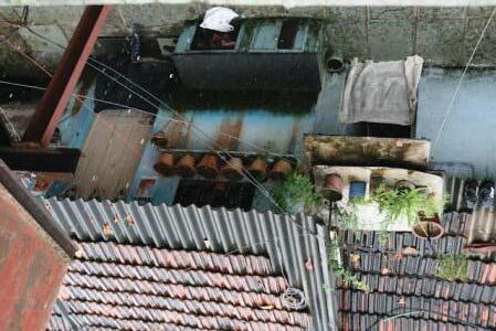
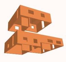
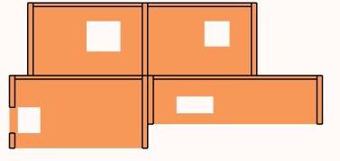
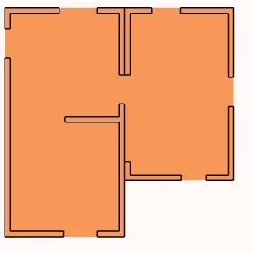
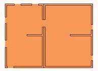
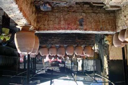
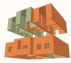
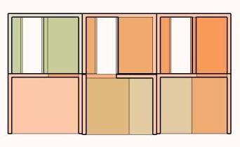
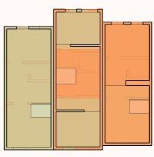
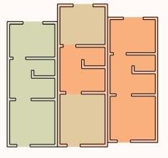
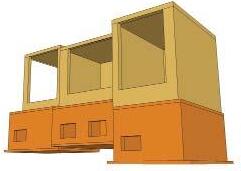
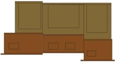
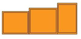
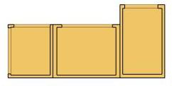
164
Residential housing type
Residential and workshop areas showing po ttery as the workshop ac tivity
Comemercial and Residential Areas
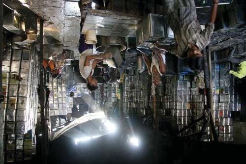
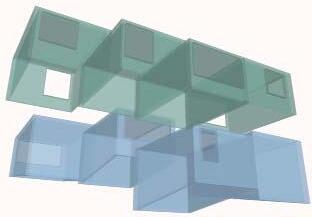
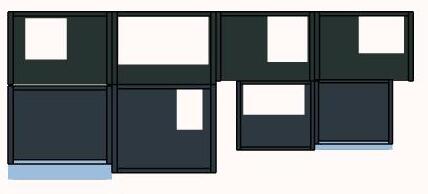
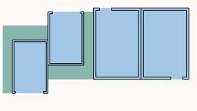
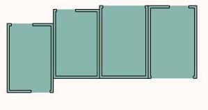
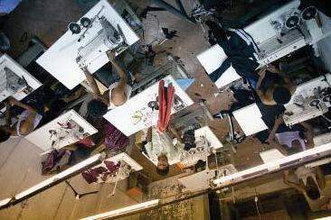
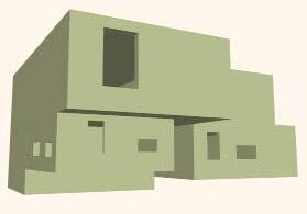
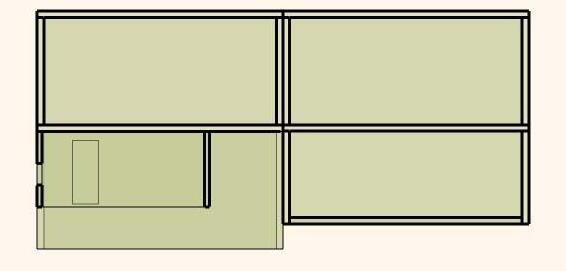
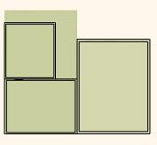
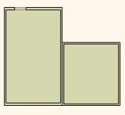
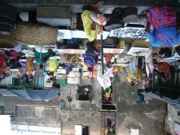
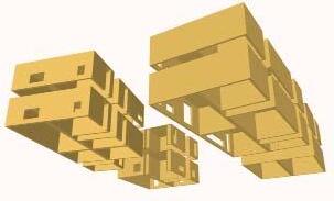
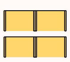
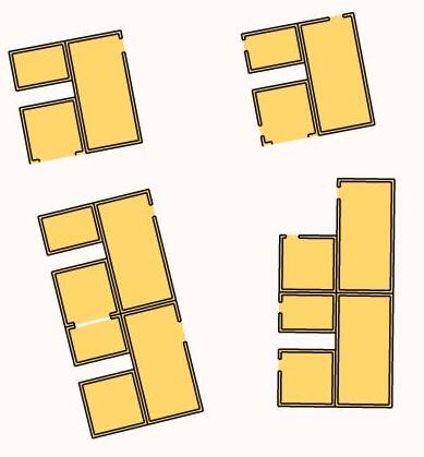
165
Small scale and Large scale workshops spaces
Large scale industrial units
Market spaces and only commercial areas
ACTIVITY TIME LINE
There is a constant overlap of programs within limited spatial boundaries based on the user needs. The space gets used for residential and workshop usage or commercial use at di fferent times of the day and year. These daily cycles reflect the need of changing spaces that adapt as per the user needs. The alongside diagram shows detailed ac tivity mappings of the di fferent program spaces depicting the space usage at di fferent times. This study was crucial during the design organization process in order to decided the placement of dynamic modules.
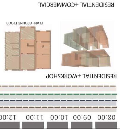
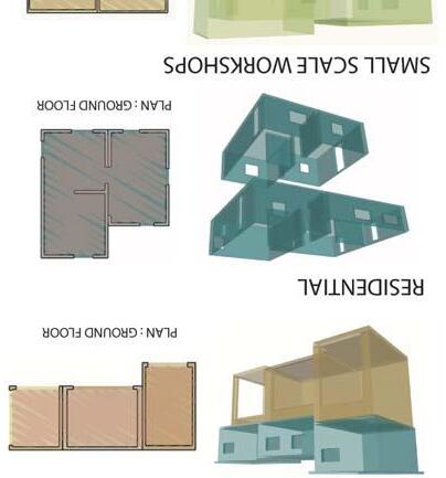
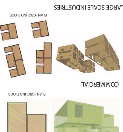
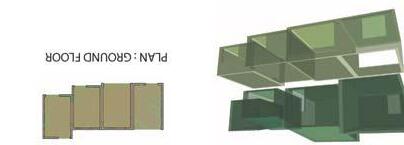
166
ACTIVITY STUDIES
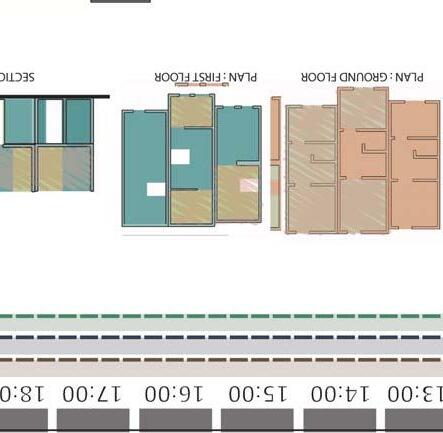
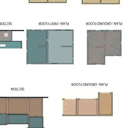
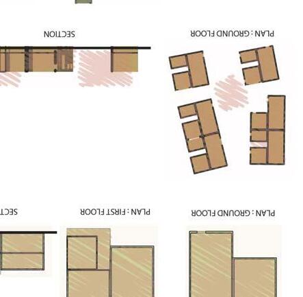
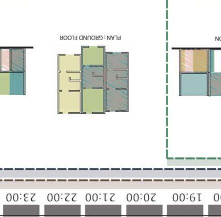
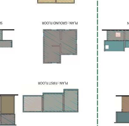
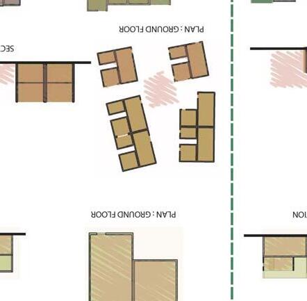
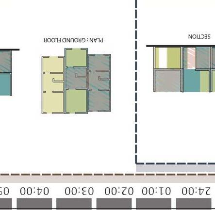
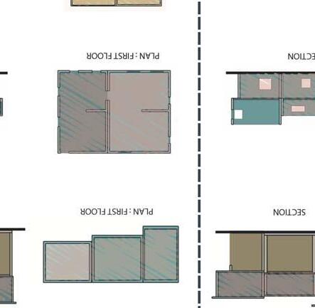
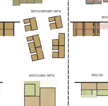
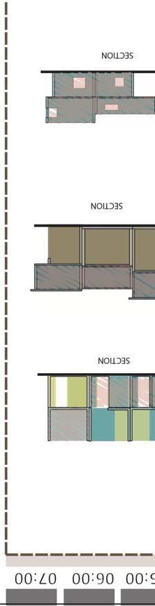
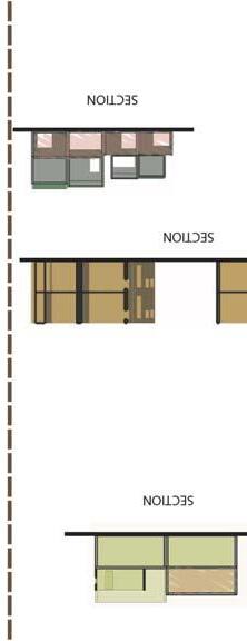
167
FABRICATION EXAMPLES
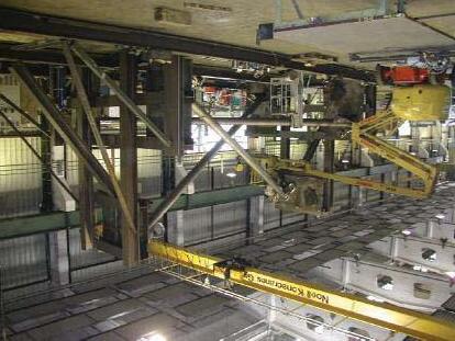
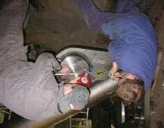
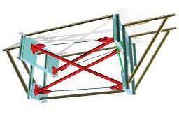
EXAMPLE OF ASSEMBY ON SITE
For the fair in Rostock (Germany) a tensegrity tower was conceived by architects Gerkan, Marg and Partners (gmp) in cooperation with engineers Schlaich, Bergermann and Partners. The modules of the tower are consisting of three compression members of about 10 m length and nine cables, six horizontal cables and three diagonal cables.
The key problem of tensegrity structures with respect to the production is the big movement of each module due to prestressing of the cables. All deflections have to be anticipated in the design of the components to eventually meet the desired geometry of the tower.
The produc tion was performed by means of a fabrication jig, where each component of one module was posi tioned with an accuracy of less than
one millimetre. The compression members were prewelded to the head plates (nodes) in the jig, removed again for full welding and assembled again in the jig for final measurement and tolerance adjustment by means of eccentric joints for the cables. The pre-stressing of the cables was performed by means of three jacks with 100 t capacity, positioned at the corner points of a triangular frame, which moved the three base points of a module inwards by about 60 mm to achieve the design prestress. The pre-stress device (frame and jacks ) remained in posi ti on for li fting of the modules, until the lower and upper nodal plates were bolted together. After erection of the lower half of the tower, the upper half was assembled on a temporary foundation and eventually li fted on top of the lower part by means of a 170 t mobile crane.
168
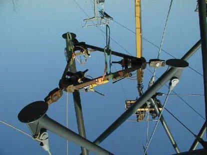
169
170
01 BIBLIOGRAPHY
02 ILLUSTRATION CREDITS
171
REFERENCES
BIBLIOGRAPHY
STRUCTURAL RESEARCH
THE MORPHOLOGY OF STRUCTURES
- By vinzenz f.j. Sedlak
Associate professor and director, lightweight structures research unit, School of architecture, the university of new south wales, sydney australia
TENSEGRITY’S SIMILARITY TO OTHER MOVEMENT SYSTEMS
- By ewald berkers
ADJUSTABLE TENSEGRITY STRUCTURES
- By Etienne Fest; Kristina Shea; Bernd Domer; And Ian F. C. Smith, M.Asce
A LITERATURE REVIEW OF TENSEGRITY
- By Brigitte servatius
COMPARING TWO DESIGN STRATEGIES FOR TENSEGRITY STRUCTURES
- By L. Rhode-barbarigos, e. Schmidt, n. Bel hadj ali and i.f.c. Smith
DRAFT: ANALYSIS OF SKEW TENSEGRITY PRISMS
- By Mark schenk
DEPLOYABLE ANTENNA KINEMATICS USING TENSEGRITY STRUCTURE DE
SIGN
By Byron franklin knight, University of florida, 2000
A PRIMER ON THE MECHANICS OF TENSEGRITY STRUCTURES
- By W. O. Williams
DEPLOYABLE TENSEGRITY STRUCTURES FOR SPACE APPLICATIONS
- By Gunnar tibert
Royal institute of technology, Department of mechanics
LIGHTNESS AND DELICACY BY CHRIS WILKINSON
- By Wilkinson eyre architects
GAIT PRODUCTION IN A TENSEGRITY BASED ROBOT
- By Chandana paul, john william roberts, hod lipson, francisco valero cuevas, Mechanical and aerospace engineering, Cornell university
DEPLOYABLE TENSEGRITY MASTS
- By A.g. Tibert, Royal institute of technology, Stockholm, sweden And S. Pellegrino, University of cambridge, Cambridge, u.k.
CLOSED-FORM EQUILIBRIUM ANALYSIS OF A PLANAR TENSEGRITY STRUCTURE
- By Jahan bayat, University of florida, Department of mechanical and aerospace engineering
- By Carl d. Crane, University of florida, Department of mechanical and aerospace engineering
STATIC ANALYSIS OF PRESTRESSED TENSEGRITY STRUCTURES
- By Carl d. Crane, University of florida, Department of mechanical and Aeronautical engineering
- By Joseph duffy, University of florida, Department of mechanical and Aeronautical engineering
- By Julio c. Correa, Universidad pontificia bolivariana, Department of mechanical Engineering
LOCOMOTION OF A TENSEGRITY ROBOT VIA DYNAMICALLY COUPLED MODULES
- By John rieffel, ryan james stuk, francisco j. Valero-cuevas and hod lipson, computational synthesis laboratory, cornell university, ithaca ny
MORPHOLOGICAL COMMUNICATION: EXPLOITING COUPLED DYNAMICS
IN A COMPLEX MECHANICAL STRUCTURE TO ACHIEVE LOCOMOTION
- By John a. Rieffel, francisco j. Valero-cuevas and hod lipson j. R. Soc.
Interface 2010 7, 613-621 first published online 23 september 2009
SYMMETRIC PRISMATIC TENSEGRITY STRUCTURES: PART I. CON¯GURATION AND STABILITY
- BY J.y. Zhang a s.d. Guest b;¤ m. Ohsaki a dept. Of architecture & architectural engineering, kyoto university, japan dept. Of engineering, university of cambridge, united kingdom
ONE-DIMENSIONAL SYNTHESIS OF GRAPHS AS TENSEGRITY Frameworks
- By András recski¤ and offer shaiy
TENSEGRITY MODULES FOR PEDESTRIAN BRIDGES
- By Landolf rhode-barbarigos*, nizar bel hadj ali a, rené motro b and ian f.c. Smith a
* applied computing and mechanics laboratory, structural engineering institute, station 18, ecole polytechnique fédérale de lausanne (epfl), lausanne ch-1015, switzerland.
Email: landolf-giosef.rhode-barbarigos@epfl.ch
A applied computing and mechanics laboratory, structural engineering institute, station 18, ecole polytechnique fédérale de lausanne (epfl), lausanne ch-1015, switzerland.
B laboratoire de mécanique et génie civil (lmgc), université de montpellier ii, montpellier cedex, france.
SYMMETRIC PRISMATIC TENSEGRITY STRUCTURES
- By J.y zhang1;2, s.d. Guest1, m. Ohsaki2
1dept. Of engineering, university of cambridge, trumpington street, cambridge cb2 1pz, united Kingdom
2dept. Of architecture and architectural engineering, kyoto university, kyoto-daigaku katsura, Nishikyo, kyoto 615-8540, japan
A SEMIDEFINITE PROGRAMMING APPROACH TO TENSEGRITY THEORY AND REALIZABILITY OF GRAPHS
-By Anthony man{cho so¤, yinyu y
STRUCTURAL MORPHOLOGY OF TENSEGRITY SYSTEMS
- By R. Motro
Asian journal of civil engineering (building and housing) vol. 10, no. 1 (2009) pages 1-19
Laboratory of mechanics and civil engineering, umrcnrs 5508, université montpellier ii, Cc048, 34095 montpellier cedex 5, france
TENSEGRITIES AND ROTATING RINGS OF TETRAHEDRA: A SYMMETRY VIEWPOINT OF STRUCTURAL MECHANICS
- By S. D. Guest phil. Trans. R. Soc. Lond. A 2000 358, 229-243
Tensegrities and rigity
Matthew thomas March 12, 2008
TENSEGRITY FRAMEWORKS: STATIC ANALYSIS REVIEW.
- By Sergi hern`andez juan 1
Institut de rob`otica i inform`atica industrial (iri), csic-upc, barcelona, spain
- By Josep m. Mirats tur 2
Institut de rob`otica i inform`atica industrial (iri), csic-upc, barcelona, spain
SHAPE CONTROL OF A MULTI AGENT SYSTEM USING TENSEGRITY STRUC TURES
-By Benjamin nabet _,1 naomi ehrich leonard _,1 _ mechanical and aerospace engineering, princeton University, princeton, nj 08544 usa, {bnabet, Naomi}@princeton.edu
THE MAKING OF A TENSEGRITY TOWER
- By Herbert klimke, soeren stephan Mero gmbh & co. Kg, max-mengeringhausen-strasse 5, d-97084 würzburg, germany
ADJUSTABLE TENSEGRITY STRUCTURES
-BY Etienne fest1; kristina shea2; bernd domer3; and ian f. C. Smith, m.sce4
AN INTRODUCTION TO THE MECHANICS OF TENSEGRITY STRUCTURES
- By Robert e. Skelton University of california, san diego
- By J. William helton University of california, san diego
- By Rajesh adhikari University of california, san diego
- By Jean-paul pinaud University of california, san diego
- By Waileung chan University of california, san diego
STABILITY CONDITIONS FOR TENSEGRITY STRUCTURES
- By J.y. Zhang, m. Ohsaki *
Department of architecture and architectural engineering, kyoto university, kyoto-daigaku katsura, nishikyo, kyoto 615-8540, japan
A PRIMER ON THE MECHANICS OF TENSEGRITY STRUCTURES
- By W. O. Williams
DEPLOYABLE ANTENNA KINEMATICS
Using tensegrity structure design
- By Byron franklin knight
REVIEW OF FORM-FINDING METHODS FOR TENSEGRITY STRUCTURES
- By A.g. Tibert and s. Pellegrino† department of structural engineering, royal institute of technology
Se-100 44 stockholm, sweden.
†department of engineering, university of cambridge Trumpington street, cambridge cb2 1pz, u.k.
ZERO STIFFNESS TENSEGRITY STRUCTURES
- By M. Schenk a, s.d. Guest b,*, j.l. Herder a
A mechanical, maritime and materials engineering, delft university of technology, mekelweg 2, 2628 cd delft, the netherlands
B department of engineering, university of cambridge, trumpington street, cambridge cb2 1pz, united kingdom
Matthew
Http://tensegrity.wikispaces.com/benefits+of+tensegrity
A RELAXATION METHOD FOR SIMULATING THE KINEMATICS OF COMPOUND NONLINEAR MECHANISMS
- By hod lipson
Sibley school of mechanical and aerospace Engineering and faculty of computing and Information, Cornell university, Ithaca, ny 14853
E-mail: hod.lipson@cornell.edu
OPTIMIZATION OF TENSEGRITY STRUCTURES
- By Milenko masic a,*, robert e. Skelton a, philip e. Gill b
A department of mechanical and aerospace engineering, university of california san diego, 9500 gilman drive, la jolla, ca 92093-0411, united states
B department of mathematics, university of california san diego, la jolla, ca 92093-0112, united states
172
TENSEGRITY STRUCTURES AND THEIR APPLICATION TO ARCHITECTURE
CHAPTER 4. DEFINITIONS AND BASIC PRINCIPLES EQUILIBRIUM CONDITIONS OF A TENSEGRITY STRUCTURE
- Proceedings of the third world conference on structural control (3wcsc) Como, italy, april 7-12, 2002 Darrell williamson, robert e. Skelton, and jeongheon han
DYNAMIC BEHAVIOR AND VIBRATION CONTROL OF A TENSEGRITY STRUCTURE
- By N. Bel hadj ali* and i.f.c. Smith Http://www.rwgrayprojects.com/synergetics/s07/p0000.html
CRAWLING BY BODY DEFORMATION OF TENSEGRITY STRUCTURE ROBOTS
- By Mizuho shibata, fumio saijyo, and shinichi hirai
KINEMATIC ANALYSIS OF TENSEGRITY STRUCTURES
- By William brooks whittier
STUDY ON TENSEGRITY ELEMENT FORM FINDING PROCESS
-By Xiaoguang Chen, Yaozhi Luo*
Dept. Of Civil Engineering, University of Waterloo, Waterloo, Ontario, N2L 3G1, Canada. X28chen@engmail.uwaterloo.ca luoyz@zju.edu.cn
STRUCTURAL PATTERNS IN NATURE – PART I
-By T. Wester
Royal Danish Academy of Fine Arts, School of Architecture, Copenhagen, Denmark Ture.wester@karch.dk
TENSEGRITY SYSTEMS. THE CASE OF POSITIVE DOUBLE CURVATURE FOR DOUBLE LAYER SYSTEMS.
-By A. Reséndiz, B. Maurin, R. Motro, N. Pauli, V. Raducanu.
SPATIALITY IN MEMBRANE STRUCTURES
-By S.L.M.C. Titotto and R.M.O. Pauletti Titotto@hotmail.com, pauletti@usp.br
TENSEGRITY GLASS STRUCTURES
- By M. Eekhout
Director Octatube Space Structures BV, Rotterdamseweg 200, 2628 AS Delft, The Netherlands
TENSION-STRUT SYSTEMS COMPOSED OF CONCENTRIC HOOPS
- By Janusz.rebielak@pwr.wroc.pl
TENSEGRITY MODULES FOR CABLE-STRUT SYSTEMS
- By A. Micheletti, V. Nicotra, P. Podio-Guidugli
THE NEW GEOMETRICAL CONCEPTION OF TENSEGRITY EXTENDER
- By Z. Bieniek
Department of Engineering Geometry and Graphics, Faculty of Civil and Environmental Engineering, Rzeszów
TWO YEARS OF TENSEGRITY MODELLING WORKSHOPS AT THE UNIVERSITY OF SHEFFIELD, SCHOOL OF ARCHITECTURE
- By Mr. Konstantinos Sakantamis1, Dr. Olga Popovic Larsen2, Mrs. E. Gutierrez3
SURFACE FITTING APPROACH FOR TENSILE MEMBRANES DESIGN
- BY J. Sánchez, M.A Serna, P. Morer
HIERARCHICAL MODULAR STRUCTURES AND THEIR GEOMETRICAL CONFIGURATIONS FOR FUTURE LARGE SPACE STRUCTURES
- By N.Kishimoto, M.C.Natori
Laboratory of Space Structures, The Institute of Space and Astronautical
TEXTEGRITY: TEXTILES AND TENSEGRITY
- BY Dr.-Ing. Lars Meeß-Olsohn Konstruktive Gestaltung, Leichtbau, Bauwesen, Universität DuisburgEssen, Universitätsstr. 15, 45141 Essen, Germany Lars.meess@uni-essen.de; www.uni-essen.de; www.leichtbaukunst.de
CABLE-STRUT GRIDS MADE OF PRISMS
- By WANG binbing and LI yanyun BLK401, Choa Chu Kang Ave 3, #10-211, Singapore 680401 Email: drbbwang@hotmail.com, li_yanyun@hotmail.com
NUMERICAL MODELLING OF TENSEGRITY SYSTEM FOLDING: PROBLEM OF COLLISIONS BETWEEN SLENDER BARS
- By C. Le Saux, F. Cevaer, R. Motro Laboratoire de Mécanique et Génie-Civil - UMR5508, Université de Montpellier II, cc048, Place E. Bataillon, 34096 Montpellier, France. Lesaux@lmgc.univ-montp2.fr, cevaer@lmgc.univ-montp2.fr, motro@ lmgc.univ-montp2.fr
VAULTED TENSEGRITY STRUCTURES: GEOMETRIC DESIGN ALGORITHMS
- By J. Kim, K.A. Liapi. Civil Engineering Department, University of Texas at Austin, 1 University Station C1752 Austin, TX 78712-0276, U.S.A. Jinman@mail.utexas.edu, kliapi@mail.utexas.edu
INVESTIGATIONS INTO THE STABILITY BEHAVIOUR OF TENSEGRITY STRUCTURES
- By K. Abedi, B. Shekastehband
Department of Civil engineering, Sahand University of Technology, Tabriz, Iran. Department of Civil engineering, Zanjan University, Zanjan, Iran. K _abedi@sut.ac.ir, shekastehband@mail.znu.ac.ir
LARGE SPAN ROOF STRUCTURES ON A SYMMETRICAL LAYOUT, CABLE DOMES OR TENSEGRITY STRUCTURES
- By L. Lazarov
STATIC AND DYNAMIC ROBUST CONTROL OF TENSEGRITY SYSTEMS
- By J.Averseng, B. Crosnier
Laboratoire de Mécanique et Génie Civil - UMR 5508, Université Montpellier II - CC 048, Place
A STUDY OF THE RESPONSE OF A CONTIGUOUS TENSEGRITY BEAM UNDER STATIC CYCLIC LOADING
- By N. Ben Kahla
Department of Mechanical Engineering, Institut Supérieur des Sciences Appliquées et de Technologie
De Sousse, Cité Taffala, 4003 Sousse Ibn Khaldoun Sousse, Tunisia.
Ph : 216 73 226 432 Fax : 216 73 332 658 Nabil.benkahla@enig.rnu.tn
AN INTELLIGENT SPATIAL TENSEGRITY STRUCTURE
- By B. Adam, I. F. C. Smith
Applied Computing and Mechanics Laboratory (IMAC) EPFL – Swiss Federal Institute of Technology in Lausanne 1015 Lausanne, Switzerland
Bernard.Adam@epfl.ch, Ian.Smith@epfl.ch
DEVELOPMENT AND REALIZATION OF A FREE–FORM TENSEGRITY STRUCTURE
- By V. Bayer1, K. Wagener2, C. Wolkowicz1 1Bauhaus – Universität Weimar, Geschwister Scholl Str. 8, D–99421Weimar, Germany. 2PWP Planungsbüro, Berlin, Germany.
PRELIMINARY REPORT OF OBSERVATION OF REAL SCALE TENSEGRITY SKELETONS UNDER TEMPERATURE CHANGE
- By K. Kawaguchi and S. Ohya Institute of Industrial Science, The University of Tokyo, Komaba 4-6-1, Meguro-ku, Tokyo 153-8505, Japan. Kawaken@iis.u-tokyo.ac.jp, ohya@iis.u-tokyo.ac.jp
NEW CONCEPT FOR DEPLOYABLE TENSEGRITY SYSTEMS STRUCTURAL MECHANISMS ACTIVATED BY SHEAR FORCES
- By Smaili A., Motro R. And Raducanu V. Laboratoire de Mécanique et Génie-Civil - UMR5508, Université de Montpellier II, cc048, Place E. Bataillon, 34096 Montpellier, France. Smaili@lmgc.univ-montp2.fr, motro@lmgc.univ-montp2.fr and vinicius. raducanu@montpellier.archi.fr
THE EXPERIMENTAL RESEARCH ON COMBINED UNIT OF FLAT-QUADRPRISM TENSEGRITY
- By Y.Z. Luo , Fu Gang , Chen Ting Space Structure Research Center of Zhejiang University, Hangzhou 310027, P.R.China Hangzhou Design Institute of Urban Construction, Hangzhou 310000, P.R.China
GRANULAR TENSEGRITY MODEL TO ANALYZE THE CYTOSKELETON ORGANIZATION IN ADHERENT CELLS
- By J. L. Milan1, S. Wendling-Mansuy1, M. Jean2, P. Chabrand1
1Laboratoire d’Aérodynamique et Biomécanique du MouvementUMSR2164, Université de la Méditerranée, 163 Avenue de Luminy, case 918, 13288, Marseille Cedex
O9, France.
2Laboratoire de Mécanique et d’Acoustique - UPR7051, 31 Chemin Joseph Aiguier, 13402 Marseille Cedex 2, France
THE CLOUD OF YVERDON
- By A. Paronesso, R. Passera Passera & Pedretti Consulting Engineers Switzerland, Via al Molino 6, CH6916 Lugano-Grancia, Switzerland.
TENSEGRITY
- By L. P.Yang, Z.B. Lin , R..J. Qian,. College of Civil Engineering, Tongji University, No.1239 Siping Road, Shanghai, China.
THE EFFECTS OF STATIC LOADING AND SUPPORT CONDITIONS ON THE PERFORMANCE OF DOUBLE LAYER VAULTED TENSEGRITY STRUCTURES
- By S.G. Liu, K.A. Liapi, J.L. Tassoulas Civil Engineering Department, University of Texas at Austin, 1 University Station C1752 Austin, TX 78712-0276, U.S.A. Richeliu@mail.utexas.edu, kliapi@mail.utexas.edu, yannis@mail.utexas.edu
173
BIOMIMETIC RESEARCH
THE ARCHITECTURE OF LIFE A UNIVERSAL SET OF BUILDING RULES SEEMS TO GUIDETHE DESIGN OF ORGANIC STRUCTURES FROM SIMPLE CAR BON COMPOUNDS TO COMPLEX CELLS AND TISSUES
- By Donald E. Ingber pg 48 Scientific American January 1998
LIFE ON THE WIRE: ON TENSEGRITY AND FORCE BALANCE IN CELLS
- By Carlo Galli1, Stefano Guizzardi, Giovanni Passeri2, Guido Maria Macaluso1, Renato Scandroglio
HOW CELLS MIGHT SENSE MICROGRAVITY DONALD INGBER1
- By Departments of Pathology & Surgery, Children’s Hospital and Harvard Medical School, Boston, Massachusetts 02115, USA
TENSEGRITY AND SPINE. A NEW BIOMECHANICAL MODEL
- By Jean Claude de Mauroy, Jean François Salmochi Clinique du Parc - Lyon (FRA)
TENSEGRITY: CONSTRUCTION OF RIGID DNA TRIANGLES WITH FLEXIBLE FOUR ARM DNA JUNCTIONS
- By Dage Liu, Mingsheng Wang, Zhaoxiang Deng, Richard Walulu, and Chengde Mao*
Department of Chemistry, Purdue UniVersity, West Lafayette, Indiana 47907
WHOLE CELL MECHANICS OF CONTRACTILE FIBROBLASTS: RELATIONS BE TWEEN EFFECTIVE CELLULAR AND EXTRACELLULAR MATRIX MODULI
- By J. Pablo Marquez, Elliot L. Elson and Guy M. Genin
NONLINEAR SYSTEMS BIOLOGY AND DESIGN: SURFACE DESIGN
- By Jenny E. Sabin, M.Arch., Lecturer, Dept of Architecture, University of Pennsylvania; Member, Institute for Medicine and Engineering; Senior Researcher, Nonlinear Systems Organization; Director, CabinStudio
ANIMAL ARCHITECTURE: BUCKMINSTER FULLER’S TENSEGRITY | REALITY SANDWICH
http://www.realitysandwich.com/animal_architecture_buckminster_fuller
HOW CELLS MIGHT SENSE MICROGRAVITY
- By DONALD INGBER1
Departments of Pathology & Surgery, Children’s Hospital and Harvard Medical School, Boston, Massachusetts 02115, USA
CPG CONTROL OF A TENSEGRITY MORPHING STRUCTURE FOR BIOMIMETIC APPLICATIONS
- By T. K. BLISS, T. IWASAKI, and H. BART-SMITH University of Virginia
Department of Mechanical and Aerospace Engineering 122 Engineer’s Way, Charlottesville, VA 22904
TENSEGRITY I. CELL STRUCTURE AND HIERARCHICAL SYSTEMS
BIOLOGY
- By Donald E. Ingber
Departments of Surgery and Pathology, Children’s Hospital and Harvard Medical School, Enders 1007, 300 Longwood Avenue, Boston, MA 02115, USA
(e-mail: donald.ingber@tch.harvard.edu)
CONTINUOUS TENSION, DISCONTINUOUS COMPRESSION A MODEL FOR BIOMECHANICAL SUPPORT OF THE BODY
- By Stephen M. Levin M.D.
http://www.intensiondesigns.com/geometry_of_anatomy.html
REVIEW PAPER: CONTINUUM BIOMECHANICS OF SOFT BIOLOGICAL TIS SUES
By J.D. Humphrey
COMPUTATIONAL RESEARCH
IMPLEMENTATION OF A COMPUTER ALGORITHM FOR AN INTERACTIVE 3D CAD GENERATION OF TENSEGRITY STRUCTURES
- By Jason E. Charalambides and Katherine A. Liapi
EVOLUTIONARY FORMFINDING OF TENSEGRITY STRUCTURES
- By Chandana Paul, Hod Lipson, Francisco Valero Cuevas Mechanical and Aerospace Engineering Cornell University Ithaca, NY 14853, USA
cp228@cornell.edu
A MARCHING PROCEDURE FOR FORM-FINDING FOR TENSEGRITY STRUCTURES
- By ANDREA MICHELETTI AND WILLIAM O. WILLIAMS
My Evolutionary Path From Tensegrity to Flextegrity, Flextegrity, Inc. 2006
AUTOMATED DISCOVERY AND OPTIMIZATION OF LARGE IRREGULAR TENSEGRITY STRUCTURES
- By John Rieffel *, Francisco Valero-Cuevas, Hod Lipson
Department of Mechanical and Aerospace Engineering, Cornell University, 138 Upson Hall, Ithaca, NY 14853, United States
REVIEW OF FORM FINDING METHODS FOR TENSEGRITY STRUCTURES
- By A.G. Tibert and S. Pellegrino†
Department of Structural Engineering, Royal Institute of Technology SE-100 44 Stockholm, Sweden.
†Department of Engineering, University of Cambridge Trumpington Street, Cambridge CB2 1PZ, U.K.
A SEMIDEFINITE PROGRAMMING APPROACH TO TENSEGRITY THEORY AND GRAPH REALIZATION
- By Anthony So
Department of Computer Science
- By Manar El–Chammas
Department of Electrical Engineering
- By Yinyu Ye
Department of Management Science and Engineering and by courtesy, Electrical Engineering
Stanford University
http://www.stanford.edu/˜yyye
174
http://www.massage-therapy-london.co.uk/Pictures/fig_6_Stellated_Tetrahedron.jpg
http://www.intensiondesigns.com
http://www.rsc.org/ej/SM/2009/b806442c/b806442c-f3.gif
http://www.thelondontraveler.com/wp-content/uploads/2008/05/skylon.jpg
http://www.gearthblog.com/images/images2006/skylon.jpg
http://en.wikipedia.org/wiki/Buckminster_Fuller
http://www.kennethsnelson.net
http://upload.wikimedia.org/wikipedia/commons/thumb/5/5d/Kenneth_Snelson_Needle_Tower.JPG/800pxKenneth_Snelson_Needle_Tower.JPG
http://farm1.static.flickr.com/148/343401788_a20365737c.jpg?v=0
http://www.slate.com/id/2093711/slideshow/2093697/
http://en.wikipedia.org/wiki/File:KurilpaBridgeConstruction5.JPG
http://www.made-in-china.com/image/2f0j00PMcawbzrJgoTM/Stainless-Steel-Expansion-Bolt-JS012-.jpg
http://www.engr.colostate.edu/ALP/images/screw-in_anchor.jpg
http://www.dywidag-systems.com/uploads/pics/DYWIDAG_Rock_Bolts_Expansion_Shell_Anchor.jpg
http://austinkids.files.wordpress.com/2008/11/snowflake2.jpg
http://www.yurtworks.co.uk/yurts/images/BakerFrame.jpg
http://upload.wikimedia.org/wikipedia/commons/4/41/Dehio_10_Dome_of_the_Rock_Sec tion.jpg
http://images.travelpod.com/users/wenzels/2.1206219600.dome-of-the-rockx-basilikax-dominus-flavit-.jpg
h tt p://chesto fb ooks.com/architecture/James-Fergusson/Illustrated-Handbook-of-Architecture---Chris ti anArchitecture/393-S.jpg
http://freepages.history.rootsweb.ancestry.com/~rgrosser/germany/dka/sanvitale.jpg
ILLUSTRATION CREDITS
175
