


©2023ZOA&HansKoster

1.Introduction (Executivesummary)
TheLivelihoodsandFoodSecurityTrustFund(LIFT)implementedprojectsandactivitiesthat supportpro-poorpolicydevelopmentandtookplacebetween2016and2020inMyanmar.It coveredthreesub-townshipsofThandaunggyiTownshipinNorthernKayinStateandwasin2019 extendedwithafewmorevillages.Theprojecttargetedover 5,000 small-holderfarmerhouseholds. Thistargetareacomprisesamixtureofdisplacedpersons,incumbenthouseholdsandreturnees withafocusonsmallholderfarmersasdirectbeneficiaries(LIFTUplandsProgrammeProject 2017).
Theprojecthelpedtheruralpoorinbothareasto“step-up”andaimedtoimprovetheirposition inthevaluechain,toimprovemarketaccessandsustainableaccesstocreditandotherfinancialand materialinputs.Oneofthemainaimsoftheprojectwastoimproveearningsofthebeneficiariesof theprogrammeastofreethemfortheviciouscycleofincreasingdebt.Nexttoimprovingearnings, theprojecthasfocusedonreducingmalnutrition,asalackofavailabilityandaccesstoadequate drinkingwaterandnutritiousfoodwasconsideredtobeaseriousissue.
Inordertoimprovelivingstandards,severalactivitiesreferredtoas outputs havebeenrolledout. Theseincludesupervisionandtrainingofmotherstoimproveknowledgeonnutrition(output1), homegardeningtrainingandinputs(output2),waterandsanitationtrainings(output3),trainings onagriculturalmethods(output4),theprovisionofagriculturalinputs(output5),improvementsto irrigationinfrastructure(output6 ),thejointconstructionofmotorcyclepathstoimproveaccessibility(output7 ),aswellasloan-and-savingstrainings(output8).Themainideaisthataconsistent setofinterlinkedactivities,trainings,andsupport,shouldimprovethelivingconditionsofthe beneficiaries.
Althoughthepremiseoftheprojectisclear,onlyexploratoryanalyseshaveshownthattheLIFT projectwaseffectiveinimprovingearningsandthenutritionofyoungchildren.However,much istobelearnedhereastheevidenceiscircumstantial,mostlyanecdotal,orbasedonqualitative methods.Thisreportaimstofillthisgapbyquantitativelyevaluatingtheimpactofthevarious activitiesundertakenunderdeumbrellaoftheLIFTproject.Wefocusonsupposedlythesingle
mostimportantoutcome–earnings(orincome).Inseveralwavesofsurveysundertakentomonitor theproject,householdswereaskedtoreporttheirannualincome.Usingmultivariateregression techniques,weinvestigatetowhatextenthouseholdsthathaveparticipatedinmoreLIFT-related activitieswitnesshigherearningsafterprojectparticipation.
Weemphasisethattheevaluationisnotbasedonanexperimentalsettingasadvocatedby, amongothers, Banerjee&Munshi (2004), Banerjee&Duflo (2011)and Banerjeeetal. (2018). Anexperimentalsettingwithatreatmentgroupandcontrolgroupisconsideredtobeidealfrom theviewpointofidentifyingcausaleffects,becausetheselectioneffectintoparticipationisfully addressed.Forexample,particularlyricherandmoreablehouseholdsmayparticipateintheseveral activitiesundertakenbytheLIFTproject.Insuchasituationonedoesnotmeasureacausaleffect oftheprogrammebutinsteadthesortingofricher/ablehouseholdsintotheproject.Unfortunately, randomisedexperimentsareusuallyverycostlyandhardtoimplementinpractice.
Still,wethinkthatwecomeascloseasreasonablypossibletoanexperimentalsettingby adoptingaso-called difference-in-differences setup(see Angrist&Pischke2008).Thisimplies thatwecompare changes inhouseholdearningsandcomparethemtothe intensity ofparticipation. Hence,weexpectthathouseholdsthatparticipatemoreintenselyinthevariousLIFTactivitieswill witnessalargerincreaseinearnings.
Adownsideofstandardquantitativemethods,includingrandomisedexperimentsanddifferencein-differencestechniques,isthatonlyan average treatmenteffectisidentified.However,wewould hopetoseethelargestincrementalchangesintheinitiallypoorhouseholds,whilehouseholds performingalreadyreasonablywellatthestartoftheprogrammearesupposedtobenefitless fromthevarioustrainingsandactivitiesoffered.Totestthishypothesis,weuseaninnovativenew methodreferredtoas UnconditionalQuantileRegressions (see Firpoetal.2009).Thistechnique enablesustoestimatetreatmenteffectsatvariouspointsintheearnings distribution.Forexample, wemayinvestigatewhethertheeffectsarelargerinthelowerendoftheearningsdistribution(i.e. forthelow-incomehouseholds).
Ideally,wewouldalsohaveinvestigatedindetailtheeffectsofthedifferentoutputs,insteadof onlyanalysingtheaggregateimpactsoftheLIFTactivities.However,itappearsthatoursample, consistingofabout 500 households,istoosmalltoobtainenoughstatisticalpowertoidentifythose effects.Indeed, LIFTUplandsProgrammeProject (2017)understandablyarguedforarelatively lownumberofhouseholdsinthesurveystosavecosts.Futureprojectsshouldprobablyincrease thesamplesizeifmoredetailontheexactworkingsoftheinvestigatedprojectiswarranted.
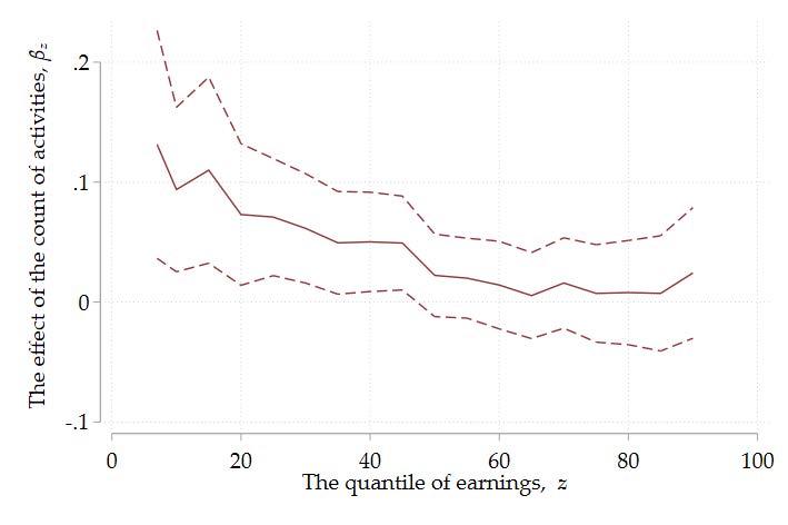
OurresultsshowthatLIFTactivitieshaveincreasedannualearnings.Theresultsindicate that,onaverage,havingparticipatedinoneoftheprogramme’sactivitiesgenerateda 3-4% higher income.Thisestimateisrobusttovariousmethodologies,includingacross-sectionalapproach withhouseholdcontrolvariablesandadifference-in-differencesapproach.Then,turningtoour heterogeneousestimates,weshowthatparticularlylow-incomehouseholdshavebenefitedfrom LIFTactivities.Theeffectforpoorhouseholdswhoareinthelowest 10% oftheearningsdistributionisabout10%,whilewedonotfindstatisticallysignificantpositiveearningseffectsfor the 50% richesthouseholdsinthesample.Hence,theLIFTprogrammeseemstohavecontributed notonlytoincreasesinearnings,butalsotoreductionsinearningsinequality.
Thisreportproceedsasfollows.InSection 2 weoutlinetheLIFTprojectandtheintended activities/outputs.Section 3 discussesthepreparationandcleaningofthedatausedfortheanalysis. Wealsoprovidesomeinitialdescriptivestatisticsforthestudiedsample.Section 4 outlinesthe methodology,whichisfollowedbytheresultsinSection 5.Section 6 concludes.
2.Projectbackgroundandprojectaims
From2016-2019ZOAwithitspartnersimplementedtheprogrammetitled‘Improvedeconomicand nutritionaloutcomeofpoorruralpeopleinMyanmar ’.ItwasaprojectfundedbytheLivelihoods andFoodSecurityFund(LIFT)andcoveredthreesub-townshipsofThandaunggyiTownship inNorthernKayinState(seeFigure 2.1).Theprojecttargetedover 5,000 smallholderfarmer households(HHs)withcommercialpotentialinThandaunggyiTownship.Thisareaemerged fromconflictandconsistsofamixtureofinternallydisplacedpersons(IDPs),IDPreturneesand incumbenthouseholds.
Theoverallpurposeoftheprojectwasformulatedas"improvedeconomicstatusandnutritional outcomesforpoorruralpeopleinMyanmarwithincreasedincomeandstableaccesstofoodfor vulnerablehouseholds".ThiswasinlinewiththepurposethatwasarticulatedbyLIFT’sUplands Programme.
Toachievethishighleveloutcomeandinconsiderationoftheneedsofthetargetgroups,the projectfocusedon (i) farmadvisoryservicesandProducerGroups, (ii) nutrition,and (iii) Social protectionandaccesstocollective/publicservices.Sustainablenaturalresourcemanagement (NRM)andGenderwereso-calledcross-cuttingissues,meaningthattheywereintegratedintoall activitiesoftheprogramme.
Thedirectaimoftheprojectwastohelptheruralpoorinthetargetedareasto‘step-up’and improvetheirpositioninthevaluechain(VC),togetaccesstomarketsandtocreditandother inputs.Besidesimprovingtheirincomeandgettingthemoutofthecircleofdebt,theproject includednutritionandWASHactivitiesasalackofavailabilityandaccesstoadequatedrinking waterandnutritiousfoodwasidentified.
ImprovedeconomicandnutritionaloutcomeofpoorruralpeopleinMyanmar wasimplemented inthenortherntownshipofKayinState,ThandaunggyiTownship(seemapbelow),andtargetsa
totalof100villages.KayinStateislocatedinthesoutheastofMyanmarandisborderedbythe MandalayRegionandShanStatetothenorth,KayahStatetothenortheast,MonStateandBago RegiontotheWest,andThailandtotheEast.
ThandaunggyiTownshipconsistsofthreesub-townships:Leikthosub-township,Thandaunggyi sub-townshipandBawgalisub-township.Therearetwotypesofvillages:Core-villagesandValue Chain-onlyvillages(VC).Core-villagesarethevillagestargetedwithallprojectcomponents.There are40core-villages.VC-onlyvillagesareonlytargetedwiththeactivitiesdescribedunderoutput 4 and5.Thereare60VC-onlyvillages.

3.Data
3.1 Datapreparation
WeuseseveralsurveysundertakentoevaluatetheLIFTproject.Thefirstisthebaselinesurvey with 373 uniquehouseholdsfrom LIFTUplandsProgrammeProject (2017),whichwasundertaken beforetheLIFTprojectstartedinthefinalquarterof2016.Thesecondsurveycapturesanother 250 householdsinearly2019.Thissecondbaselinesurveywasundertakenbecauseanothersetof villageswasaddedtothe 40 corevillagesinthesample(see LIFTUplandsProgrammeProject 2019).Thenwehavetwo‘endline’surveysaftertheprojectfinishedcapturing 393 householdsfor theinitialvillagesand250forthevillagesaddedin2019.

Foreachofthesesurveys,wekeepthevariablesthatareconsistentlymeasuredacrossthe differentwavesinourdata.Thekey outcome variableofinterestisannualearnings,which ismeasuredinMyanmareseKyat(i.e. Ks.10,000 isabout$4 80).Onemaybeworriedthat earningsaremeasuredwitherror,becauseearningsareselfreported.Fortunately,asearningsisour dependentvariable,withrandommeasurementerror,theestimatedeffectsarenotimpacted(see Koster&VanOmmeren2020).Wethinkitisreasonabletoassumerandommeasurementerror becausepeopleareunlikelytomakesystematicerrorsinreportingtheirearnings.
Toconstructourmain treatment variable,wecountthetypeofactivitiesahouseholdparticipates inineachstudyperiod,whichishalfayear.Forexample,ahouseholdmayhaveparticipatedin mothergroupseninhavereceivedtrainingsonagriculturalmethodsinthefirsthalfof2017.Then, thetreatmentvariableisequalto 2.Alternatively,weconsidertocountthefrequencyofactivities.
Forexample,ahouseholdmayhaveparticipated 5 timesinmothergroups,andhasfollowed 3 activitiesrelatedtobusinessgroups.Then,thisalternativetreatmentvariableequals 8.Werefer totheformvariableas countofactivitiesparticipated,whiletothelattervariableas frequencyof activitiesparticipated.
Further,wehaveinformationonthevillagewherethehouseholdlives,whichenablesusto latercontrolfortrendsintheproductivityofcertainvillages.Fromthesurveys,wealsoobtain informationontheethnicgroupwheretheheadofthehouseholdbelongsto,aswellasthereported religion,whethertherespondentismarried,ownsland,andisafarmer.Usingahouseholdidentifier wecantracehouseholdsovertimetoseehowearningshavedeveloped.Becausewethinkitis unlikelythatethnicityorreligionchanges,wetaketheethnicityandreligionfromthebaseline surveyforeachhousehold.
3.2 Descriptivestatistics
Inthissubsectionwefurtherillustratethecharacteristicsofthedata.InTable 3.1 weshowwhatwe calldescriptivestatisticsforthedependentvariableandthecontrolvariables.Weshowrepresent themean,standarddeviation(i.e. thespread),minimumandmaximumvaluespervariable.Thisis usefultoseeifthereareanyoutliervalues.Theaverageannualearningsinthefirstbaselinesurvey from2016areKs. 909 thousand,whichisabout$ 430,whichisonly$ 1 18 perday.Thisclearly indicatesthathouseholdsinthissurveyandparticipatinginthesupportprogrammeareverypoor. Thespread,however,issubstantial.Thehouseholdwiththehighestearningsisabout$ 4 thousand peryear.Theaverageearningsconsiderablyincreasedovertheyears.Inthefinalsurvey,average earningshaveincreasedbyalmost50%toKs.1 3million(approximately$620)
Lookingatthecontrolvariables,mostparticipantsaremarried(about 95%).Almostalwaysthe headofthehouseholdismale(alsoabout 95%).Further,almostallhouseholdsownlandthatthey useforagriculturalactivities.Further,mosthouseholdsareChristian,withBaptistsandCatholics beingthelargestgroups.However,pleasenotethattheshareofBaptisthouseholdsisconsiderably largerinthefirstbaselinesurvey,ascomparedtothesecondbaselinesurvey.Themostdominant ethnicgroupisKebaKaren(respectively36%and77%inthefirstandsecondbaselinesurvey).
InTable 3.2 weshowthedescriptivesoftheparticipationinvariousactivities(i.e. outputs).For completeness,weshowalsothefirstbaseline.Obviously,asthefirstbaselinesurveytookplace beforeanyactivitieswherelaunched,allvariablesequalzero.Asthesecondbaselinesurveytook placeearly2019,householdsalreadyparticipatedinvariousactivities.Asnotallactivitieswere rolledoutinthevillagesthatwerepartofthesecondbaseline,theoutputs 1, 2 and 3 areequalto zero.
WethinkPanelCinTable 3.2 isthemostinteresting.Onaverage,householdsattheend ofthesampleperiodparticipatedinalmost 8 different activities,whicharecountedeachhalfa year.Despitethesecondbaselinegroupnotparticipating,thefirstoutput,providingknowledge onnutritiontomothers,hasthehighestparticipationacrosshouseholds.Therearehouseholds thathaveparticipatedalotinvariousactivities,asthemaximumis 25.Otheractivitiesthathave highparticipationratesareoutput4(trainingonagriculturalmethods)andoutput5(provisionof agriculturalinputs).Wealsoreportthefrequencyofparticipatinginactivities.Onehousehold hasparticipatedinastunningnumberof 109 activities.Weseethatthefrequencyofactivitiesis dominatedbyoutput1(knowledgeonnutrition)andoutput2(homegardeningandinputs).
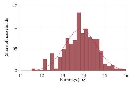
Next,wewillinvestigateinFigure 3.1 whetherthemainvariablesofinterestarenormally
3.1–D ESCRIPTIVESTATISTICS : DEPENDENTVARIABLEANDCONTROLS
Notes: Thenumberofobservationsindefirstbaselineis348,itis248inthesecondbaselineand623inthe endlinesurvey.
TABLE 3.2–D ESCRIPTIVESTATISTICS : TREATMENTVARIABLES
PANEL
distributed.InFigure 3.1a weshowthedistributionofearningsinthefirstbaselinesurvey.Because earningsarelikelyaso-calledskeweddistribution,wetakethelogarithmofearnings(see Koster& VanOmmeren2020).Itisshownthatthedistributionismoreorlesslog-normallydistributed.
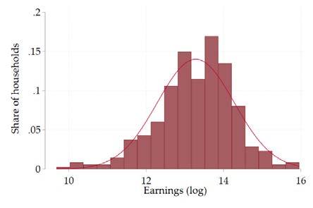
Figure 3.1b showsthedistributionofearningsfortheendlinesurvey,whichisagainmoreor lesslog-normallydistributed.Pleasenotethatthedistributionshiftedtotherightcomparedtothe baselineearningsdistribution,whichisinlinewiththestrongaverageincreaseinearningsbetween thebaselineandendlinesurveyofabout50%.
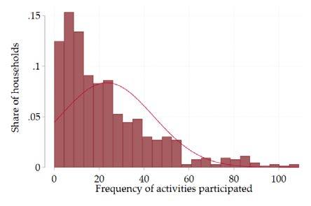
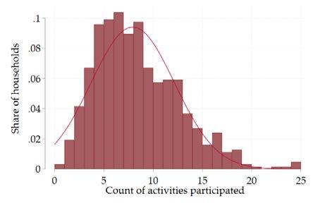
InFigure 3.1c weshowthecountofactivitiesparticipated.Itismoreorlessnormallydistributed, apartfromafewoutliersbeyond 20 activities.Pleasenotethatwecannottaketheloghere,because thecountofactivitiescanbezero(whichisparticularlytrueforthefirstbaselinesurvey)andone cannottakethelogarithmofzero.
Finally,thefrequencyofactivities(seeFigure 3.1d)isstronglyskewed.Wethereforepreferto focusonthecountofactivitiesasthemaintreatmentvariabletoavoidtheissuethatoutliershavea disproportionateimpactontheresults.Still,wewillprovideancillaryanalyseswhereweanalyse theimpactofthefrequencyofactivitiesonearnings.
4.Methodology

4.1 Amultivariateregressionapproach
Astandardwaytoinvestigatetheimpactofatreatmentorindependentvariableonanoutcomeor dependentvariableistoestimatelinearregressions.1 Usually,therelationshipbetweentreatment variableandoutcomevariablesisdescribedbyasimpleequationofthefollowingform:
where yivt aretheannualearningsofhousehold i livinginvillage v intime t and civt isthecount ofactivitiesthatthehouseholdsparticipatedinsofar.Thelattercorrespondstoeitherthefirst baselinesurvey,thesecondbaselinesurveyortheendlinesurvey.Further, α and β areregression parameterstobeestimated,while εivt istheresidual,orthepartofearningsthatwecannotexplain by civt .
Pleasenotethat β hereisthekeyparameterofinterestanddepictswhathappenstoearnings,in percentageterms,ifthecountofactivitiesincreasesby 1.Say,forexample,that β = 0 01,thenfor eachactivitythehouseholdparticipatedin,theannualearningsincreaseby1%.
However,theabovemodelislikelyatoosimplisticdescriptionofrealityasnotonlythe countofactivitieshasanimpactonearnings,butalsotheethnicity,religion,andmaritalstatus ofthehousehold,aswellasthevillagewherethehouseholdlivesdeterminesincome.Iffor examplehouseholdswithacertainethnicityorreligionhavehigherearnings and participatemore inactivities,wemayfalselyattributetheimpactofethnicityandreligiontothetreatmentvariable.
1 Inlinearregressions,therelationshipbetweenthetreatmentvariable(s)andoutcomevariablearemodelledusing linearpredictorfunctionswhoseunknownmodelparametersareestimatedfromthedata.Itappearsthatthebestlinear unbiasedestimatorofthecoefficientofinterest–sotheimpactofthetreatmentvariableontheoutcomevariable–is obtainedbyminimisingthesquaredresiduals.
Toaddressthisissueitisimportantto control forhouseholdandlocationcharacteristicsthatmay alsodeterminetheearningsofthehousehold.Anextendedequationthenlooksasfollows:
log yivt = α + β civt + γ xivt + δv + εivt , (4.2)
where xivt arecontrolvariables,suchasethnicityandreligion,and γ isasetofparameterscapturing theimpactsofthesevariablesonearnings.Wealsoincludeso-calledvillage fixedeffects,denoted by δv .Thisimpliesthatweincludeadummyvariableforeachvillageastocontrolforfactors influencinghouseholds’earningsatthevillagelevelthatarethesameforeveryone.Forexample, somevillagesmayhavebetteraccesstofertilegrounds,whichwillleadtohigheryieldsandinturn higherearnings.Byincludingthesevillagefixedeffectswecontrolforallthosefactors.
4.2 Addressingtheselectioneffect
Amajorconcernwiththeaboveapproachisthepresenceofapotentialselectioneffect Angrist &Krueger (2001), Angrist&Pischke (2008).Thisselectioneffectentailsthathouseholdsthat haveahigherearningspotentialaremorelikelytoparticipatein(many)activitiesoffered.Hence, inthisway,wedonotmeasurethecausaleffectoftheintervention,butinsteadcapturethefact thathouseholdsthatwouldhaveexperiencedhigherearningsgrowthabsentoftheprogramme participatemoreintenselyintheactivitiesoffered.
Acommonsolutionistoapplyrandomisation,meaningthatthetreatment(i.e.,theactivities offered)israndomisedacrosshouseholds.Randomisationobviouslyaddressestheselectioneffect becausehouseholdcouldnotself-selectintotheprogramme Angrist&Pischke (2008).
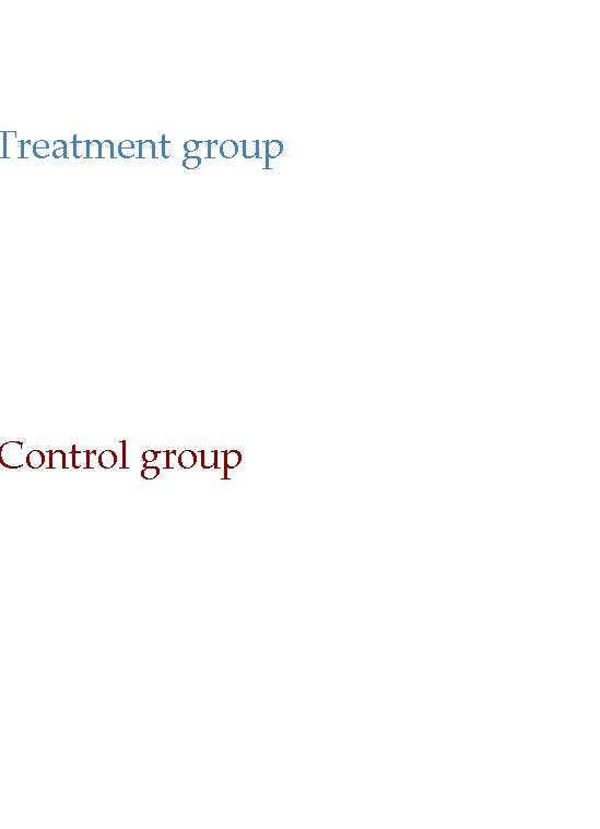
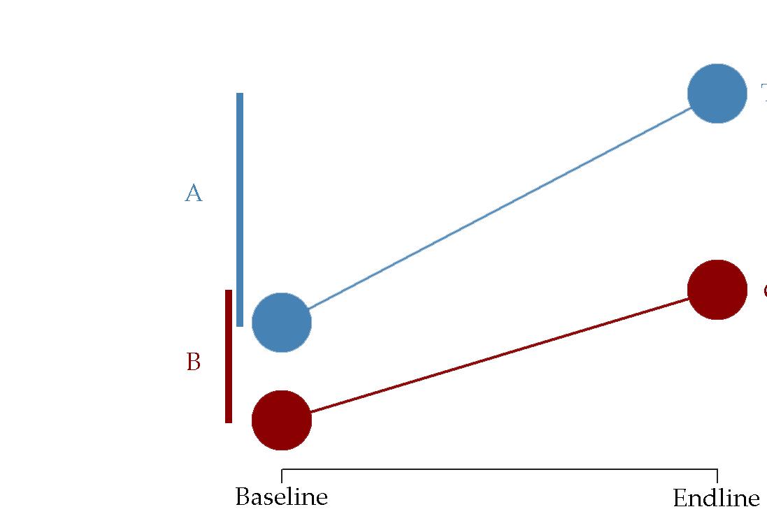
Unfortunately,wecannotrelyonrandomisationinthecurrentsettingbecauseparticipationin theactivitieswasvoluntary.Instead,weuseaversionofanapproachthatisoftenusedinapplied economics,whichisreferredtoasthe difference-in-differences (DID)approach(Bertrandetal. 2004, Angrist&Pischke2014).WeprovideanexampleofthismethodinFigure 4.1.Theideais thefollowing:oneshouldhaveobservationsofanoutcomevariable(inourcase:earnings)before andaftertreatment.Assumethatacertaingroupofhouseholdsdoesnotreceivetreatment.Absent ofthetreatment,thosepeoplewitnessanincreaseinearningsof B.Thentherearethehouseholds thatreceivetreatment.InFigure 4.1 itcanbeseenthatthosehouseholdsinitiallyhavehigher earnings(i.e.,haveahigherbaselineearningslevel).However,thisisnotanissuebecausewe lookatthechangeinearningsovertime,whichisequalto A.Whatisthenthecausaleffectofthe treatment?Well,thatis A B,becauseabsentofthetreatmentthetreatmentgroupwouldhave experiencedanincreaseinearningsequalto B sothe additional effectofthetreatmenteffectis equalto A B
Inoursettingweonlyhaveveryfewhouseholdsthatdidnotparticipateinanyoftheactivities. However,wecanusethe intensity oftreatmenttocomparechangesinearnings.Hence,ifwe comparethedifferencesinthetrendshouseholdsthathaveparticipatedin2versus1activities,we cantracetheeffectofattendingoneextraactivity.
Formally,theapplicationofthisDIDapproachisstraightforward:wejustincludeso-called
household fixedeffects,whichareessentiallydummyvariablesforeachhousehold:
log yivt = α + β civt + γ xivt + ζi + εivt , (4.3) where ζi capturesthehouseholdfixedeffects.Theinclusionofhouseholdfixedeffectsensurethat wecontrolforbaselinedifferencesinearningsacrosshouseholdsandonlyusevariationinthe trendsinearningsoftimeacrosshouseholds.
Onestillmaybeconcernedthatdifferentvillagesmaybeondifferenttrends,implyingthat,for example,duetochangesinclimaticconditionssomevillagesmayfacelowergrowthinearnings.If thesechangesinclimaticconditionsarecorrelatedtothetreatment,ourestimate β isstillbiased. Toaddressthisissue,inafinalspecificationweincludevillage-by-yearfixedeffectstoabsorball trendsinearningsatthevillagelevel:
log yivt = α + β civt + γ xivt + δvt + ζi + εivt , (4.4) where δvt capturesvillage-by-yearfixedeffects.
4.3 Allowingforheterogeneityinthetreatmenteffect
Thedifference-in-differencedesignisusefulinidentifyingthe average effectofthetreatment. Inmanyapplications,however,oneisinterestedinheterogeneityinthetreatmenteffectacross households.Inoursettingweareparticularlyinterestedwhetherhouseholdsthatareinitiallypoor haveexperiencedlargerbenefitsfromtheprogrammethaninitiallyslightlyricherhouseholds.A veryusefulrecentinnovationtodisentangletheseeffectsiswhat Firpoetal. (2009)refertoas unconditionalquantileregressions.Thismethodallowsustomeasurethetreatmenteffectateach quantileoftheearningsdistribution.Quantilesarecutpointsdividingtherangeoftheearnings distributionintocontinuousintervalswithequalprobabilities.Hence,alowerquantilemeansthata householdhaslowearnings(i.e. isontheleftsideofFigures 3.1a or 3.1b),whileahigherquantile
4.3Allowingforheterogeneityinthetreatmenteffect 17
meansthatahouseholdisrelativelyricher(i.e. isontherightsideofFigures 3.1a or 3.1b).2
Itisgenerallyconvenienttoapplyunconditionalquantileregressionsbecauseitisshownby Firpoetal. (2009)thatthisjustentailsatransformationofthedependentvariable, log yivt ,bymeans ofaso-calledrecenteredinfluencefunction(RIF).Weaimtoestimatethefollowingspecification:
where RIF ( ) istheRIFforagivenquantile z ofearningsand βz capturestheeffectofinterestfor agivenquantile z oftheearningsdistribution.
2 Letusgiveanexample.Saywehavedataon 100 householdsandwerangethesehouseholdswithearningsfrom hightolow.Then,thefirstobservationsissaidtobethefirstquantileoftheearningsdistribution,the 50th quantileisthe middleobservation,whichisalsocalledthemedian,whilethe 100th quantileisthehouseholdwiththehighestearnings inourdata.