
Chapter 3: Describing, Exploring, and Comparing Data
Section 3-1: Measures of Center
1. The term average is not used in statistics. The term mean should be used for the result obtained by adding all of the sample values and dividing the total by the number of sample values.
2. No. The 50 amounts are all weighed equally in the calculation that yields the mean of 19.67, but some states have higher smoking rates, so the mean smoking rate should be calculated using a weighted mean that takes into account the smoking rates in the different states.
3. They use different approaches for providing a value (or values) of the center or middle of the sorted list of data.
4. Using the five values,
Using the six values, including the outlier of
The outlier caused the mean to change by a substantial amount, but the median changed very little. The median is resistant to the effect of the outlier, but the mean is not resistant.
5.
Apart from the fact that the other charges are lower than those given, nothing meaningful can be known about the population of all charges.
The measures of center do not provide any information about the change of MCAT scores over time.
is 799 53.0. 11
The jersey numbers are nominal data that are just replacements for names, and they do not measure or count anything, so the resulting statistics are meaningless.
The median is 225.0 lb.
modes are 190 lb and 305 lb.
8. (continued)
The midrange is 189305 247.0 2
All of the weights are from players on only one of the 32 NFL teams, but it isn’t likely that any of the teams has weights that are substantially different from those of any other team, so it is reasonable to conclude that the weights are somewhat representative of all NFL players.
The median is 2.0.
The mode is 1.
The midrange is 14 2.5. 2
The mode of 1 correctly indicates that the smooth-yellow peas occur more than any other phenotype, but the other measures of center do not make sense with these data at the nominal level of measurement.
The mode is $1500.
The sample consists of “best buy” TVs, so it is not a random sample and is not likely to be representative of the population. The lowest price is a relevant statistic for someone planning to buy one of the TVs.
11.
If concerned about radiation absorption, you might purchase the cell phone with the lowest absorption rate. All of the cell phones in the sample have absorption levels below the FCC maximum of 1.6 W/kg.
12. The mean is
The median is 3841
The mode is 0 mg.
The midrange is 055 27.5 2 mg.
Americans consume some brands much more often than others, but the 20 brands are all weighted equally in the calculations, so the statistics are not necessarily representative of the population of all cans of the same 20 brands consumed by Americans.
13. The mean is
The median is 1820 19.0 2 firefighters.
The modes are 15 and 20 firefighters.
The midrange is 834 21.0 2 firefighters.
Copyright © 2018 Pearson Education, Inc.
13. (continued)
The data are time series data, but the measures of center do not reveal anything about a trend consisting of a pattern of change over time.
14.
Because the measurements were made in 1988, they are not necessarily representative of the current population of all Army women.
15.
Apart from the fact that all other colleges have tuition and fee amounts less than those listed, nothing meaningful can be known about the population.
16.
The median is 0.0 cigarettes. The mode is 0 cigarettes.
Because the selected subjects report the number of cigarettes smoked, it is very possible that the data are not at all accurate. And what about that person who smokes 50 cigarettes (or 2.5 packs) a day? What are they thinking?
17.
Given that systolic and diastolic blood pressures measure different characteristics, a comparison of the measures of center doesn’t make sense. Because the data are matched, it would make more sense to investigate whether there is an association or correlation between systolic blood pressure measurements and diastolic blood pressure measurements.
Copyright © 2018 Pearson Education, Inc.
18. (continued) Red
Because the data are matched, it would make more sense to investigate whether there is an association or correlation between white and red blood cell counts.
19.
Females appear to have higher white blood cell counts.
20. Single Line:
Individual lines: same results as with a single line. Although the mean and median are the same, the times with individual lines are much more varied than those with a single line.
21. Using all values, the mean is 53.7 mg/dL x and the median is 52.0 mg/dL. The highest value of 138 mg/dL appears to be an outlier. Excluding 138 mg/dL, the mean is 53.4 mg/dL x and the median is 52.0 mg/dL. Excluding the outlier does not cause much of a change in the mean, and the median remains the same.
22. Using all values, the mean is 113.7 mg/dL x and the median is 113.0 mg/dL. The highest value of 251 mg/dL appears to be an outlier. Excluding 251 mg/dL, the mean is 113.3 mg/dL x and the median is 113.0 mg/dL. Excluding the outlier does not cause much of a change in the mean, and the median remains the same.
23. The mean is 98.20F x and the median is 98.40F. These results suggest that the mean is less than 98.6F.
24. The mean is 3152.0 x g and the median is 3300 g. All of the weights end in 00, so they are all rounded to the nearest 100 grams. This suggests that the results should be rounded as follows: 3150.0 x g and the median is 3300 g.
29. a. The missing value is
beats per minute. b.
30. The mean ignoring the presidents who are still alive is 15.0 years. The mean including the presidents who are still alive is at least 15.7. years. The results do not differ by a considerable amount.
31. Mean: 113.7 mg/dL; 10% trimmed mean: 112.6 mg/dL; 20% trimmed mean: 112.2 mg/dL. The 10% trimmed mean and 20% trimmed mean are both fairly close, but the untrimmed mean of 113.7 mg/dL differs from them because it is more strongly affected by the outliers.
Section 3-2: Measures of Variation
1. 3 1439963 119.0 cm, 4 s which is quite close to the exact value of the standard deviation of 124.9 cm3
2. Significantly low values are less than or equal to 3 1126.02(124.9)876.2 cm and significantly high values are greater than or equal to 3 1126.02(124.9)1375.8 cm.
A brain volume of 1440 cm3 is significantly high. 3.
2 20.0414 kg401.6577 kg
5. The range is 471,062155,857$315,205.0.
(Many technologies will not provide all of the digits shown for the variance 2 , s so any result close to the value shown here is acceptable.) Because only the 10 highest sample values are used, nothing much can be known about the population of all such charges.
6. The range is 28.426.81.60.
The standard deviation is 0.3240.57. s
The results do not provide any information about the change of MCAT scores over time.
7. The range is 99792.0.
The standard deviation is
The jersey numbers are nominal data that are just replacements for names, and they do not measure or count anything, so the resulting statistics are meaningless.
8. The range is 305189116.0
The standard deviation is
lb. All of the weights are from players on only 1 of the 32 teams, but it isn’t very likely that any of the teams has weights that are substantially different from those of any other team, so it is reasonable to conclude that the measures of variation are typical of NFL players.
9. The range is 413.0.
The standard deviation is 0.90.9. s
The measures of variation can be found, but they make no sense because the data don’t measure or count anything. They are nominal data.
10. The range is 1800950$850.0.
The sample consists of “best buy”
so it is not a random sample and is not likely to be representative of the population. The measures of variation are not likely to be typical of all TVs that are 60 inches or larger.
11. The range is 1.490.510.980 W/kg.
No. Some models of cell phones have a much larger market share than others, so the measures from the different models should be weighted according to their size in the population.
12. The range is 55055.0 mg.
The standard deviation is 2 413.420.3 s
mg.
Americans consume some brands much more often than others, but the 20 brands are all weighted equally in the calculations, so the statistics are not necessarily representative of the population of all cans of the same 20 brands consumed by Americans.
13. The range is 34826.0 firefighters.
The variance is
2 2 145770264 60.9 14141 s firefighters2.
The standard deviation is 60.97.8 s firefighters.
The data are time-series data, but the measures of variation do not reveal anything about a trend consisting of a pattern of change over time.
14. The range is 10.48.61.80 in.
The variance is
The standard deviation is 0.270.52 s in. Because the measurements were made in 1988, they are not necessarily representative of the current population of all Army women.
15. The range is 57,26153,323$3938.0.0.
The variance is
The standard deviation is 1,638,970.9$1280.2. s
Because the data include only the 10 highest costs, the measures of variation don’t tell us anything about the variation among costs for the population of all U.S. college tuitions.
16. The range is 50050.0 cigarettes.
The variance is
The standard deviation is 89.79.5 s cigarettes. Because the selected subjects report the number of cigarettes smoked, it is very possible that the data are not at all accurate, so the results might not reflect the actual smoking behavior of California adults.
17. Systolic: 127.6, x 18.6; s The coefficient of variation is 18.6 100%14.6%. 127.6
Diastolic: 73.6, x 12.5; s The coefficient of variation is 12.5 100%16.9%. 73.6
The variation is roughly about the same.
18. All units are 1000 cells/L.
White Blood Cell Counts: 6.73, x 1.46; s The coefficient of variation is 1.46 100%21.7%. 6.73
Red Blood Cell Counts: 4.57, x 0.42; s The coefficient of variation is 0.42 100%9.2%. 4.57 White blood cell counts appear to vary more than red blood cell counts.
19. All units are 1000 cells/L.
Male: 6.17, x 1.53; s The coefficient of variation is 1.53 100%24.8%. 6.17
Female: 7.35, x 1.57; s The coefficient of variation is 1.57 100%21.3%. 7.35
The variation is roughly about the same.
20. Single Line: 429.0, x 28.6; s The coefficient of variation is 28.6 100%6.7%. 429.0
The coefficient of variation is 109.3
The single line has much less variation than with individual lines. 21. Using all data:
substantial amounts.
24. 22 Range4600.0g, 480,848.1g, 693.4g; ss
All of the weights end in 00, so they are all rounded to the nearest 100 grams. This suggests that the results should be rounded as follows: 22 Range4600.0g, 480,850g, 690g. ss
25. The rule of thumb standard deviation is
found by using all of the data.
26. The rule of thumb standard deviation is
found by using all of the data.
27. The rule of thumb standard deviation is
which is much larger than
mg/dL s
which is not substantially different from 0.62F s
found by using all of the data.
28. The rule of thumb standard deviation is
which differs from 693.4 s g found by using all of the data by a considerable amount. Several of the lowest weights correspond to premature births, and they cause the range to be larger, with the resulting estimate being larger.
29. Significantly low values are less than or equal to
beats per minute, and significantly high values are greater than or equal to
beats per minute. A pulse rate of 44 beats per minute is significantly low.
30. Significantly low values are less than or equal to
beats per minute, and significantly high values are greater than or equal to
69.6211.392.2
beats per minute. A pulse rate of 50 beats per minute is neither significantly low or high.
31. Significantly low values are less than or equal to 77.3221.2924.74
cm, and significantly high values are greater than or equal to
77.3221.2929.90
cm. A foot length of 30 cm is significantly high.
32. Significantly low values are less than or equal to 98.2020.6296.96F,
and significantly high values are greater than or equal to 98.2020.6299.44F.
A body temperature of 100F is significantly high.
Copyright © 2018 Pearson Education, Inc.
b. The nine possible samples of two values are the following: {(9, 9), (9, 10), (9, 20), (10, 9), (10, 10), (10, 20), (20, 9), (20, 10), (20,20)} which have the following corresponding sample variances:{0, 0.5, 60.5, 0.5, 0, 50, 60.5, 50, 0}, that have a mean of 2 2.47 s cigarettes2.
c. The population variances of the nine samples above are {0, 0.25, 30.25, 0.25, 0, 25, 30.25, 25, 0} that have a mean of 2 12.3 s cigarettes2
d. Part (b), because repeated samples result in variances that target the same value (24.7 cigarettes2) as the population variance. Use division by 1. n
e. No. The mean of the sample variances (24.7 cigarettes2) equals the population variance (24.7 cigarettes2), but the mean of the sample standard deviations (3.5 cigarettes) does not equal the population standard deviation (5.0 cigarettes).
36. The mean absolute deviation of the population is 4.7 cigarettes. With repeated samplings of size 2, the nine different possible samples have mean absolute deviations of 0, 0, 0, 0.5, 0.5, 5, 5, 5.5, 5.5. With many such samples, the mean of those nine results is 2.4 cigarettes, showing that the sample mean absolute deviations tend to center about the value of 2.4 cigarettes instead of the mean absolute deviation of the population, which is 4.7 cigarettes. The sample mean deviations do not target the mean deviation of the population. This is not good. This indicates that a sample mean absolute deviation is not a good estimator of the mean absolute deviation of a population.
Section 3-3: Measures of Relative Standing and Boxplots
1. James’ height is 4.07 standard deviations above the mean.
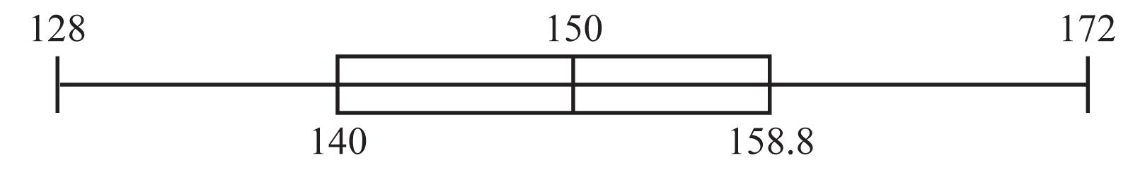
2. The minimum height is 155 cm, the first quartile, 1,Q is 169.1 cm, the second quartile, 2,Q (or the median) is 173.8 cm, the third quartile, 3,Q is 179.4 cm, and the maximum height is 193.3 cm.
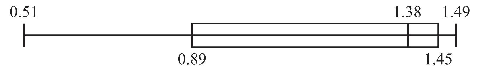
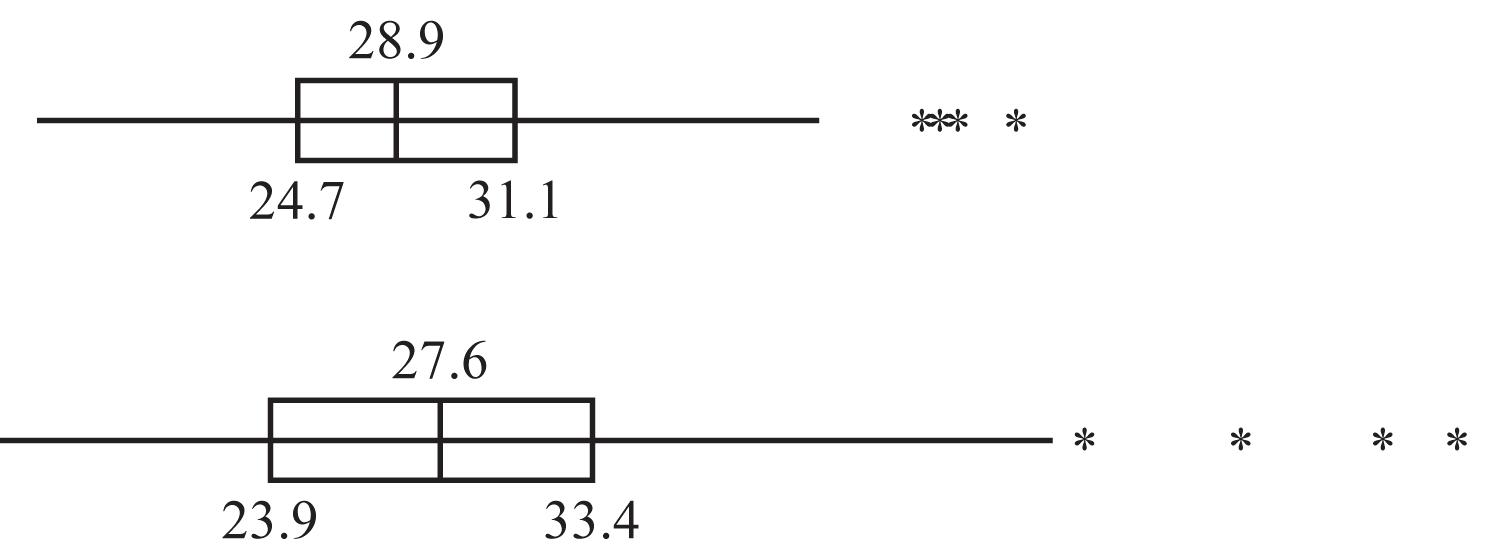
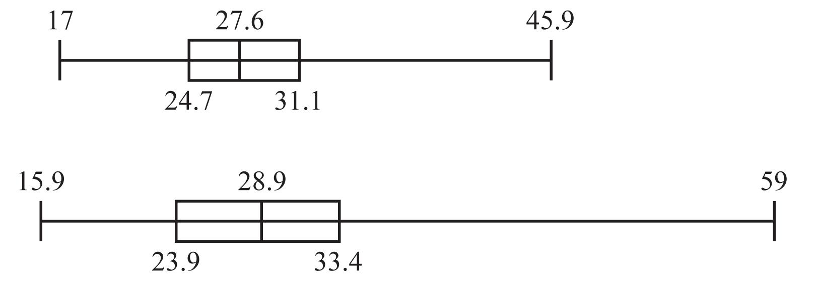
3. The bottom boxplot represents weights of women, because it depicts weights that are generally lower.
4. 2.00 should be preferred, because it is 2.00 standard deviations above the mean and would correspond to the highest of the five different possible scores.
5. a. The difference is 1047430 bpm.
b. 30 2.74 12.5 standard deviations
c. 2.74 z
d. The pulse rate of 104 beats per minute is significantly high.
6. a. The difference is 367438 BPM.
b. 38 3.04 12.5 standard deviations
c. 3.04 z
d. The pulse rate of 36 beats per minute is significantly low.
7. a. The difference is 96.5098.201.7F.
b. 1.7 2.74 0.62 standard deviations
c. 2.74 z
d. The temperature of 96.5F is significantly low.
8. a. The difference is 98.6098.200.4F.
b. 0.4 0.65 0.62 standard deviations
c. 0.65 z
d. 3Q is not significantly high.
9. Significantly low scores are less than or equal to
and significantly high scores are greater than or equal to
21.125.131.3.
10. Significantly low scores are less than or equal to
and significantly high scores are greater than or equal to
25.226.438.0.
11. Significantly low weights are less than or equal to
g, and significantly high weights are greater than or equal to
12. Significantly low hip breadths are less than or equal to
cm, and significantly high hip breadths are greater than or equal to
13. The tallest man’s z score is
the shortest man’s
Chandra Bahadur Dangi has the more extreme height because his z score of –16.83 is farther from the mean than the z score of 10.83 for Sultan Kosen.
14. The female has a higher red blood cell count because her z score is
which is a higher number than the z score of
for the male.
15. The male has a more extreme birth weight because his z score is
which is a lower number than the z score of
for the female.
16. Julianne Moore had the more extreme age since her z score is
which is farther from the mean than the z score of 3344.1 1.25 8.9 z for Eddie Redmayne.
Copyright © 2018 Pearson Education, Inc.
17. For

, so it is the 17th percentile.
, so it is the 50th percentile. 18. For
, so it is the 81st percentile.
Copyright © 2018 Pearson Education, Inc.
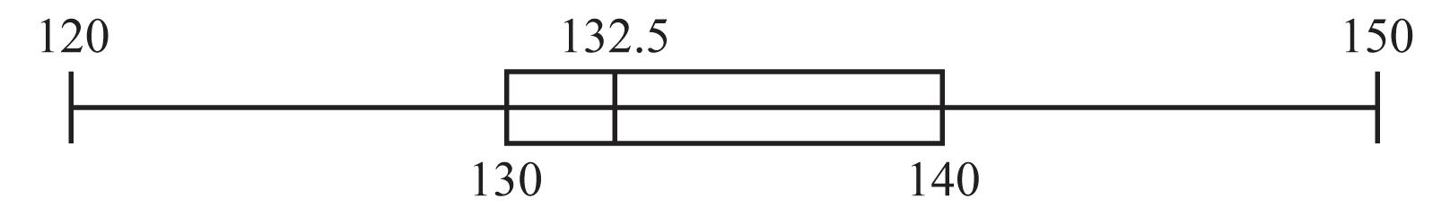
32. The five number summary is 120 mm Hg, 130.0 mm Hg, 132.5 mm Hg, 140.0 mm Hg, 150 mm Hg.
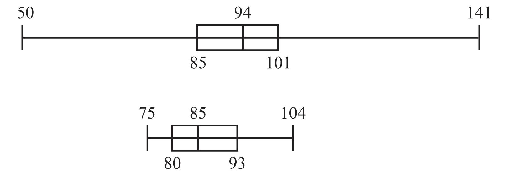
33. The top boxplot represents BMI values for males. The two boxplots do not appear to be very different, so BMI values of males and females appear to be about the same, except for a few very high BMI values for females that caused the boxplot to extend farther to the right.
34. The low lead level group represented in the top boxplot has much more variation and the IQ scores tend to be higher than the IQ scores from the high lead level group.
35. Bottom boxplot represents females. The two boxplots are not dramatically different. The outliers for females are 48.0 in., 52.6 in., 56.8 in., and 59.0 in. The outliers for males are 43.2 in., 43.7 in., 44.2 in., 45.9 in.
Chapter Quick Quiz
2. The median is 77 7.0
3. The modes are 7 hours and 8 hours.
4. The variance is 22 (1.3 hours) = 1.7 hours
5. Yes, because 0 hours is substantially less than all of the other data values. 6.
Copyright © 2018 Pearson Education, Inc.
7. 75% or 60 sleep times
8. minimum, first quartile Q1, second quartile Q2 (or median), third quartile Q3, maximum
9. 104 1.5 4 s
hours
1. a. The mean is 1497+1538+1550+1571+1642 1559.6 mm.
b. The median is 1550.0 mm.
c. There is no mode.
d. The midrange is 14971642 1569.5 mm. 2
e. The range is 16421497145.0 mm.
g. 222 53.42849.3 mm s
2. 16421559.6 1.54; 53.4 z
The eye height is not significantly low or high because its z score is between 2 and –2, so it is within 2 standard deviations of the mean.
3. The mean is 1214222740 23.0. 5 x
The numbers don’t measure or count anything. They are used as replacements for the names of the categories, so the numbers are at the nominal level of measurement. In this case the mean is a meaningless statistic.
4. The male z score is 34003273 0.19 660 z . The female z score is 32003037 0.23 706 z . The female has the larger relative birth because the female has the larger z score.
5. The outlier is 646. The mean and standard deviation with the outlier included are 267.8 x and 131.6. s With the outlier excluded, the values are 230.0 x and 42.0. s Both statistics changed by a substantial amount, so here the outlier has a very strong effect on the mean and standard deviation.
6. The minimum value is 119 mm, the first quartile is 128 mm, the second quartile (or median) is 131 mm, the third quartile is 135 mm, and the maximum value is 141 mm.
7. Significantly low heights are 97.526.983.7 cm or less; significantly high heights are 111.3 cm or greater. The height of 97.526.987.8 cm is not significant, so the physician should not be concerned.
8. The median would be better because it is not affected much by the one very large income.
Cumulative Review Exercises
Copyright © 2018 Pearson Education, Inc.
5. a. Mode, because the others are numerical measures that require data at the interval or ratio levels of measurement.
b. convenience sampling
c. More consistency can be achieved by lowering the standard deviation. (It is also important to keep the mean at an acceptable level.)