WL2017R16_011_1.pdf by Vlaanderen-be

www.ﬂandershydraulicsresearch.be16_011_1FHRreportsUncertainty in wave overtopping calculation using SWASH Shallow foreshore conditions (along the Flemish coast)

Uncertainty in wave overtoppingusingcalculationSWASH Shallow foreshore conditions (along the Flemish coast) De Roo, S.; Suzuki, T.; Altomare, C.; Mostaert, F.

F WL PP10 2 Version 6 Valid as from Cover1/10/2016figure © The Government of Flanders, Department of Mobility and Public Works, Flanders Hydraulics Research 2017 Legal FlandersnoticeHydraulics Research is of the opinion that the information and positions in this report are substantiated by the available data and knowledge at the time of writing. The positions taken in this report are those of Flanders Hydraulics Research and do not reflect necessarily the opinion of the Government of Flanders or any of its institutions. Flanders Hydraulics Research nor any person or company acting on behalf of Flanders Hydraulics Research is responsible for any loss or damage arising from the use of the information in this report. Copyright and citation © The Government of Flanders, Department of Mobility and Public Works, Flanders Hydraulics Research 2017 ThisD/2017/3241/257publicationshould be cited as follows: De Roo, S.; Suzuki, T.; Altomare, C.; Mostaert, F. (2017). Uncertainty in wave overtopping calculation using SWASH: Shallow foreshore conditions (along the Flemish coast). Version 4.0. FHR Reports, 16_011_1. Flanders Hydraulics Research: Antwerp Until the date of release reproduction of and reference to this publication is prohibited except in case explicit and written permission is given by the customer or by Flanders Hydraulics Research. Acknowledging the source correctly is always CustomerDocumentmandatory.identification:Agentschap Maritieme Dienstverlening en Kust Afdeling Kust Ref.: WL2017R16_011_1 Keywords (3 5): Hydraulic boundary conditions, wave overtopping, numerical modelling, safety assessment Text (p.): 68 Appendices (p.): 51 Confidentiality: ☒ Yes Released as from: 01/01/2020 Author(s): De Roo, S.; Suzuki, T.; Altomare, C. Control

To assess this variability in wave overtopping, 500 simulations were carried out for every case In total, 18 cases were identified by categorizing the Flemish coastline into 6 generalized bathymetric configurations, varying in cross shore profile, in foreshore length, in presence of a steeper part in its slope closer to the dike and ending in a dike, have a 1:2 slope and 3 different crest levels.

The number of waves overtopping a structure is governed by the number of large wave heights in the wave train and the specific sequence of waves arriving at the structure. Hence, random wave trains resulting from the same energy density spectrum, lead possibly to different volumes of waves that overtop and introduce variability in the numerically estimated wave overtopping discharge

To conclude, wave overtopping discharge needs to be estimated by at least 8 SWASH 1D simulations. Their mean result is then the wave overtopping discharge on which for seed number selection and sample size uncertainty needs to be accounted for, in order to obtain a final numerical estimate of the wave overtopping discharge.

OffshoreAbstractwaveboundary conditions often consist of energy density spectra being readily available (e.g. offshore wave buoys) or idealized energy density spectra of which the parameters are reported (e.g. in the Hydraulic Boundary Condition book, De Roo et al., 2016) In numerical modelling, an infinite number of surface elevation time series can be generated out of one energy density spectrum by linearly superposing the spectral wave components, of which the phases are assumed to be randomly distributed. To create randomly varying phase components, an input seed number is needed By varying this seed number for every simulation, a different surface elevation time series, i.e. different wave train, will be created.

Final version WL2017R16_011_1 III

Given that wave overtopping discharge is accepted to be normally distributed, its mean result and the variability around this value can be assessed by its relative error. The higher the mean wave overtopping discharge, the lower the relative error becomes (power law relation). Indeed, the higher the freeboard, the smaller the probability of overtopping, and hence, the more wave overtopping depends on the individual wave characteristics in the surface elevation time series. Translating this fitted relation to a confidence band around the mean indicates that 68.3% of the wave overtopping values are captured within ± 1 standard deviation around the mean. The upper confidence limit, generally used for design and assessment purposes, adds some safety to the mean result, and hence, the mean wave overtopping result needs to be increased by its associated standard deviation to account for seed number variability. In practice, it is not possible to carry out that amount of simulations to determine the wave overtopping discharge. Applying both a Monte Carlo and data sampling approach, the added uncertainty was quantified given that only a reduced sample of 1 to 20 wave overtopping estimates is used instead of 500. As from a sample size of 8, the added accuracy gained by increasing the sample size becomes insignificant compared to the calculation effort of doing extra simulations. Therefore, a sample size of 8 is opted for.

Uncertainty in wave overtopping calculation using SWASH Shallow foreshore conditions (along the Flemish coast)

Uncertainty in wave overtopping calculation using SWASH Shallow foreshore conditions (along the Flemish coast) Final version WL2017R16_011_1 V AbstractContents III Contents V List of figures VII List of tables ...................................................................................................................................................... XI 1 Introduction ............................................................................................................................................... 1 1.1 Background ........................................................................................................................................ 1 1.2 Objective ............................................................................................................................................ 1 1.3 Reader’s guide through the document ............................................................................................. 2 2 Literature review ....................................................................................................................................... 3 2.1 Wave overtopping in case of (very) shallow foreshores 3 2.2 Wave overtopping equations 4 2.3 (Numerical) modelling of wave overtopping 6 2.4 The use of SWASH 1D for wave overtopping 7 3 Bathymetries along the Flemish coast 9 3.1 Sources of post storm bathymetric data 9 3.1.1 XBEACH 9 3.1.2 DUROSTA 9 3.2 Categorized bathymetries ................................................................................................................. 9 3.3 Generalization of categorized bathymetries ................................................................................... 13 4 SWASH model train ................................................................................................................................. 15 4.1 2D wave transformation .................................................................................................................. 15 4.1.1 Setup ........................................................................................................................................ 15 4.1.2 Results: incident hydraulic boundary conditions at the toe of the dike 15 4.2 1D calibration of wave transformation 24 4.2.1 Setup 24 4.2.2 Results: calibration 24 4.2.3 Results: incident hydraulic boundary conditions at the toe of the dike 27 4.3 1D wave overtopping 38 4.3.1 Setup 38 4.3.2 Numerical instability 38 4.3.3 Results: wave overtopping ...................................................................................................... 40 4.3.4 Results: statistical distribution of wave overtopping data ...................................................... 44

Uncertainty in wave overtopping calculation using SWASH Shallow foreshore conditions (along the Flemish coast) VI WL2017R16_011_1 Final version 5 Wave overtopping ................................................................................................................................... 45 5.1 Influence of boundary conditions ................................................................................................... 45 5.2 Results: SWASH vs. empirical equations ......................................................................................... 47 6 Uncertainty reduction in wave overtopping calculation using SWASH 53 6.1 Uncertainty source 1: calibration mismatch 53 6.3 Uncertainty source 2: seed number 56 6.4 Uncertainty source 3: sample size 59 6.5 Using SWASH for wave overtopping calculation: accounting for uncertainty sources 63 7 Conclusion & outlook 64 7.1 Conclusion 64 7.2 Outlook further research .............................................................................................................. 65 8 References ............................................................................................................................................... 67 Appendix 1: Sources of post storm bathymetries ........................................................................................... A1 Appendix 2: Wave overtopping: descriptive statistics ................................................................................. A2 Appendix 3: Wave overtopping: mean and standard deviation against sample size .................................. A51

Figure 15

Figure 16 Seed dependent calibration of the still water level SWLoff

................................ 37 Figure 27 Mean

Error bars indicate the

Figure 18 Seed dependent wave set up in relation to the offshore still water level SWLoff

(one

Seed dependent calibration of the significant wave height Hm0,off

.... 35 Figure 25

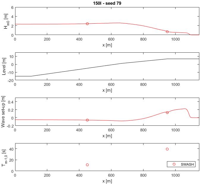
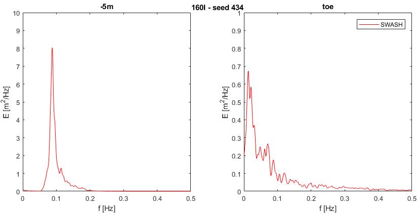
Figure Case 150I wave parameters and spectra at 5m TAW and toe of the dike (seed 12345079) Case 160I wave parameters and spectra at 5m TAW and toe of the dike (seed 12345434)

Uncertainty in wave overtopping calculation using SWASH Shallow foreshore conditions (along the Flemish coast) Final version WL2017R16_011_1 VII List of figures Figure 1 General post storm bathymetry of the Westkust (Coastal section 25) 11 Figure 2 General post storm bathymetry of the Middenkust (Coastal section 103) 11 Figure 3 General post storm bathymetry of the Oostkust (Coastal section 233) 12 Figure 4 Coastal section 115: a beach nourishment is carried out, which stops storm induced erosion at a certain distance from the dike (Durosta calculation, Ruiz Parrado et al., 2016)............................................ 12 Figure 5 Generalized post storm bathymetries ............................................................................................ 14 Figure 6 Mean incident significant wave height Hm0 at the toe of the dike. Error bars indicate the standard deviation (n = 300 except for 260: n = 291).................................................................................................... 16 Figure 7 Mean spectral wave period Tm 1,0 at the toe of the dike. Error bars indicate the standard deviation (n = 300 except for 260: n = 291) .................................................................................................................... 16 Figure 8 Mean wave set up at the toe of the dike. Error bars indicate the standard deviation (n = 300 except for 260: n = 291)................................................................................................................................... 17 Figure 9 Case 200I wave parameters and spectra at 5m TAW and toe of the dike (seed 12345140) ...... 18 Figure 10 Case 210I wave parameters and spectra at 5m TAW and toe of the dike (seed 12345140) .... 19 Figure 11 Case 230I wave parameters and spectra at 5m TAW and toe of the dike (seed 12345140) .... 20 Figure 12 Case 240I wave parameters and spectra at 5m TAW and toe of the dike (seed 12345140) 21 Figure 13 Case 250I wave parameters and spectra at 5m TAW and toe of the dike (seed 12345140) 22 Figure 14 Case 260I wave parameters and spectra at 5m TAW and toe of the dike (seed 12345140) 23

Figure incident significant wave height Hm0 at the toe of the dike for the 2 calibration setups. the standard deviation (one seed: n = 500; all seeds: n cf. Table 5) spectral wave period Tm 1,0 at the toe of the dike for the 2 calibration setups. standard deviation seed: n = 500; all seeds: n cf. Table 5)

26 Mean

.... 33

Error bars indicate

Figure 19

................................................. 37

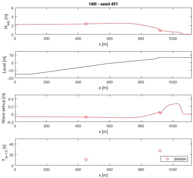
Figure Case 140I wave parameters and spectra at 5m TAW and toe of the dike (seed 12345451)

Figure

Seed dependent significant wave height Hm0,toe and associated spectral wave period Tm 1,0,toe at the toe of the dike

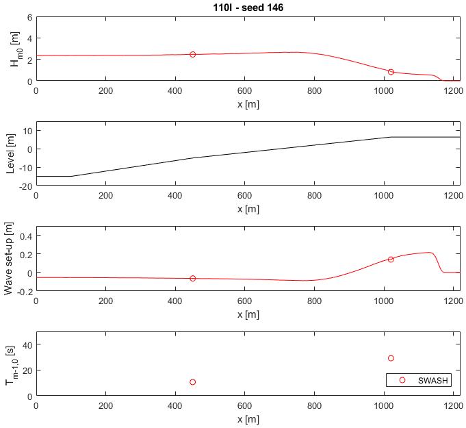
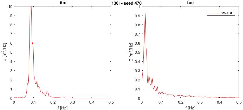
Figure 20 Case 100I wave parameters and spectra at 5m TAW and toe of the dike (seed 12345261) Case 110I wave parameters and spectra at 5m TAW and toe of the dike (seed 12345146) Case 130I wave parameters and spectra at 5m TAW and toe of the dike (seed 12345470)

.... 31 Figure 21

.... 32 Figure 22

.... 36

Seed dependent wave set up in relation to the offshore significant wave height Hm0,off

.... 34

Uncertainty in wave overtopping calculation using SWASH Shallow foreshore conditions (along the Flemish coast) VIII WL2017R16_011_1 Final version Figure 28 Mean wave set up at the toe of the dike for the 2 calibration setups. Error bars indicate the standard deviation (one seed: n = 500; all seeds: n cf. Table 5) ..................................................................... 38 Figure 29 Mean wave overtopping discharge (error bars indicate the standard deviation). ....................... 41 Figure 30 Zoom on mean wave overtopping discharge (excluding case 143) (error bars indicate the standard deviation). ........................................................................................................................................ 41 Figure 31 Boxplots of wave overtopping discharge q (one seed calibration) ............................................... 42 Figure 32 Zoom on boxplots of wave overtopping discharge q (excluding case 143; one seed calibration) 42 Figure 33 Boxplots of wave overtopping discharge q (seed dependent calibration) 43 Figure 34 Zoom on boxplots of wave overtopping discharge q (excluding case 143; seed dependent calibration) 43 Figure 35 Wave steepness sm 1,0 for all cases 46 Figure 36 Ratio between the water depth dtoe and incident wave height Hm0,toe at the toe of the dike for all cases 46 Figure 37 Dimensionless wave overtopping discharge Qdim in relation to the relative freeboard Rc* 47 Figure 38 Input wave overtopping equations: wave steepness sm 1,0 and average slope m 49 Figure 39 Dimensionless wave overtopping discharge Qdim results: SWASH vs. empirical equation 1 (using coefficient of eq 5: ‘MB’) 50 Figure 40 Dimensionless wave overtopping discharge Qdim results: SWASH vs. empirical equation 1 (using coefficient of eq 6: ‘Alto’) 51 Figure 41 Ratio of wave overtopping discharge Qdim between SWASH and equation eqdet 5 in relation to the dimensionless wave overtopping discharge modelled by SWASH 52 Figure 42 Ratio of wave overtopping discharge q, calculated by equation, given a perfect and real calibrated match of incident hydraulic boundary conditions in relation to the dimensionless wave overtopping discharge Qdim modelled by SWASH 55 Figure 43 Mean wave overtopping �� in relation to its relative error σ’ (seed dependent calibration) 57 Figure 44 Mean wave overtopping q and its 68% and 90% confidence bands (black: seed dependent calibration; grey: one seed calibration) ......................................................................................................... 57

discharge modelled

Figure overtopping characteristics: mean and standard deviation against sample size for Monte Carlo (MC) data sampling (DS red: reduced number of samples = 100)

1 (including

methods

45 Probabilistic

and

62 Figure 50 Relation

Figure and deterministic ratio of wave overtopping discharge Qdim between SWASH and equation coefficients of eq 5: ‘eqMB’) in relation to the dimensionless wave overtopping and deterministic ratio of wave overtopping discharge Qdim between SWASH and equation 1 (including coefficients of eq 6: ‘eqAlto’) in relation to the dimensionless wave overtopping by SWASH Carlo (B and and data sampling (A and C) methods: wave overtopping characteristics

49 Standard

Figure deviation on wave overtopping discharge against sample size for Monte Carlo (MC) data sampling (DS red: reduced number of samples = 100): cases 10X and 15X between mean and standard deviation of wave overtopping discharge sample size:

48 Wave

discharge modelled by SWASH 58 Figure 46 Probabilistic

8 ......................................................................................................................................................................... 62

59 Figure 47 Monte

related to sample size 60

Uncertainty in wave overtopping calculation using SWASH Shallow foreshore conditions (along the Flemish coast) Final version WL2017R16_011_1 IX Figure 51 Histogram of the wave overtopping data of case 101 .................................................................. A3 Figure 52 Normal Q Q plot of wave overtopping data of case 101 .............................................................. A3 Figure 53 Histogram of the ln(wave overtopping) data of case 101 ............................................................. A4 Figure 54 Rankits Q Q plot of the ln(wave overtopping) data of case 101 A5 Figure 55 Histogram of the wave overtopping data of case 102 A6 Figure 56 Normal Q Q plot of the wave overtopping data of case 102 A6 Figure 57 Histogram of the wave overtopping data of case 103 A7 Figure 58 Normal Q Q plot of the wave overtopping data of case 103 A8 Figure 59 Histogram of the wave overtopping data of case 111 A9 Figure 60 Normal Q Q plot of the wave overtopping data of case 111 A9 Figure 61 Histogram of the ln(wave overtopping) data of case 111 ........................................................... A10 Figure 62 Normal Q Q plot of the ln(wave overtopping) data of case 111 ................................................. A11 Figure 63 Histogram of the wave overtopping data of case 112 ................................................................ A12 Figure 64 Normal Q Q plot of the wave overtopping data of case 112 ...................................................... A12 Figure 65 Histogram of the ln(wave overtopping) data of case 112 ........................................................... A13 Figure 66 Normal Q Q plot of the ln(wave overtopping) data of case 112 A14 Figure 67 Histogram of the wave overtopping data of case 113 A15 Figure 68 Normal Q Q plot of the wave overtopping data of case 113 A15 Figure 69 Histogram of the ln(wave overtopping) data of case 113 A16 Figure 70 Normal Q Q plot of the ln(wave overtopping) data of case 113 A17 Figure 71 Histogram of the wave overtopping data of case 131 A18 Figure 72 Normal Q Q plot of the wave overtopping data of case 131 A18 Figure 73 Histogram of the ln(wave overtopping) data of case 131 A19 Figure 74 Normal Q Q plot of the ln(wave overtopping) data of case 131 ................................................. A20 Figure 75 Histogram of the wave overtopping data of case 132 ................................................................ A21 Figure 76 Normal Q Q plot of the wave overtopping data of case 132 ...................................................... A21 Figure 77 Histogram of the ln(wave overtopping) data of case 132 ........................................................... A22 Figure 78 Normal Q Q plot of the ln(wave overtopping) data of case 132 ................................................. A23 Figure 79 Histogram of the wave overtopping data of case 133 ................................................................ A24 Figure 80 Normal Q Q plot of the wave overtopping) data of case 133 ..................................................... A24 Figure 81 Histogram of the ln(wave overtopping) data of case 133 A25 Figure 82 Normal Q Q plot of the ln(wave overtopping) data of case 133 A26 Figure 83 Histogram of the wave overtopping data of case 141 A27 Figure 84 Normal Q Q plot of the wave overtopping data of case 141 A27 Figure 85 Histogram of the wave overtopping data of case 142 A28

Uncertainty in wave overtopping calculation using SWASH Shallow foreshore conditions (along the Flemish coast) X WL2017R16_011_1 Final version Figure 86 Normal Q Q plot of the wave overtopping data of case 142 ...................................................... A29 Figure 87 Histogram of the wave overtopping data of case 143 ................................................................ A30 Figure 88 Normal Q Q plot of the wave overtopping data of case 143 ...................................................... A30 Figure 89 Histogram of the ln(wave overtopping) data of case 143 A31 Figure 90 Normal Q Q plot of the ln(wave overtopping) data of case 143 A32 Figure 91 Histogram of the wave overtopping data of case 151 A33 Figure 92 Normal Q Q plot of the wave overtopping data of case 151 A33 Figure 93 Histogram of the ln(wave overtopping) data of case 151 A34 Figure 94 Normal Q Q plot of the ln(wave overtopping) data of case 151 A35 Figure 95 Histogram of the wave overtopping data of case 152 A36 Figure 96 Normal Q Q plot of the wave overtopping data of case 152 ...................................................... A36 Figure 97 Histogram of the ln(wave overtopping) data of case 152 ........................................................... A37 Figure 98 Normal Q Q plot of the ln(wave overtopping) data of case 152 ................................................. A38 Figure 99 Histogram of the wave overtopping data of case 153 ................................................................ A39 Figure 100 Normal Q Q plot of the wave overtopping data of case 153 .................................................... A39 Figure 101 Histogram of the ln(wave overtopping) data of case 153 A40 Figure 102 Normal Q Q plot of the ln(wave overtopping) data of case 153 A41 Figure 103 Histogram of the wave overtopping data of case 161 A42 Figure 104 Normal Q Q plot of the wave overtopping data of case 161 A42 Figure 105 Histogram of the ln(wave overtopping) data of case 161 A43 Figure 106 Normal Q Q plot of the ln(wave overtopping) data of case 161 A44 Figure 107 Histogram of the wave overtopping data of case 162 A45 Figure 108 Normal Q Q plot of the wave overtopping data of case 162 A45 Figure 109 Histogram of the ln(wave overtopping) data of case 162 ......................................................... A46 Figure 110 Normal Q Q plot of the ln(wave overtopping) data of case 162............................................... A47 Figure 111 Histogram of the wave overtopping data of case 163 .............................................................. A48 Figure 112 Normal Q Q plot of the wave overtopping data of case 163 .................................................... A48 Figure 113 Histogram of the ln(wave overtopping) data of case 163 ......................................................... A49 Figure 114 Normal Q Q plot of the ln(wave overtopping) data of case 163............................................... A50

Uncertainty in wave overtopping calculation using SWASH Shallow foreshore conditions (along the Flemish coast) Final version WL2017R16_011_1 XI List of tables Table 1 Schematisation of the categorized bathymetries 13 Table 2 Offshore hydraulic boundary conditions (RT= 1000 year, CS 105 in De Roo et al., 2016) 15 Table 3 Calibration criteria to be met concurrently for the incident hydraulic boundary conditions at the toe of the dike 24 Table 4 Results for setup 1: calibration of seed 12345001 ........................................................................... 25 Table 5 Success rate for setup 2: calibration of 500 individual seed numbers ............................................. 25 Table 6 Number of instable wave overtopping simulations using one seed calibration (between brackets) and seed dependent calibration input values ................................................................................................. 39 Table 7 Selected 1D simulations having a perfect calibration match of incident hydraulic boundary conditions to the 2D results ............................................................................................................................ 54 Table 8 Calibrated offshore hydraulic boundary conditions for 130I ............................................................. 54 Table 9 Difference in the SWASH and equation wave overtopping results given 2 perfect calibration matches ........................................................................................................................................................... 55 Table 10 Sources of post storm bathymetries .............................................................................................. A1 Table 11 Tests of normality for wave overtopping data of case 101 ............................................................ A2 Table 12 Tests of normality for ln(wave overtopping) data of case 101 A4 Table 13 Tests of normality for wave overtopping data of case 102 A5 Table 14 Tests of normality for wave overtopping data of case 103 A7 Table 15 Tests of normality for wave overtopping data of case 111 A8 Table 16 Tests of normality for ln(wave overtopping) data of case 111 A10 Table 17 Tests of normality for wave overtopping data of case 112 A11 Table 18 Tests of normality for ln(wave overtopping) data of case 112 A13 Table 19 Tests of normality for wave overtopping data of case 113 A14 Table 20 Tests of normality for ln(wave overtopping) data of case 113..................................................... A16 Table 21 Tests of normality for wave overtopping data of case 131 .......................................................... A17 Table 22 Tests of normality for ln(wave overtopping) data of case 131..................................................... A19 Table 23 Tests of normality for wave overtopping data of case 132 .......................................................... A20 Table 24 Tests of normality for ln(wave overtopping) data of case 132..................................................... A22 Table 25 Tests of normality for wave overtopping data of case 133 .......................................................... A23 Table 26 Tests of normality for ln(wave overtopping) data of case 133 A25 Table 27 Tests of normality for wave overtopping data of case 141 A26 Table 28 Tests of normality for wave overtopping data of case 142 A28 Table 29 Tests of normality for wave overtopping data of case 143 A29

Uncertainty in wave overtopping calculation using SWASH Shallow foreshore conditions (along the Flemish coast) XII WL2017R16_011_1 Final version Table 30 Tests of normality for ln(wave overtopping) data of case 143..................................................... A31 Table 31 Tests of normality for wave overtopping data of case 151 .......................................................... A32 Table 32 Tests of normality for ln(wave overtopping) data of case 151..................................................... A34 Table 33 Tests of normality for wave overtopping data of case 152 A35 Table 34 Tests of normality for ln(wave overtopping) data of case 152 A37 Table 35 Tests of normality for wave overtopping data of case 153 A38 Table 36 Tests of normality for ln(wave overtopping) data of case 153 A40 Table 37 Tests of normality for wave overtopping data of case 161 A41 Table 38 Tests of normality for ln(wave overtopping) data of case 161 A43 Table 39 Tests of normality for wave overtopping data of case 162 A44 Table 40 Tests of normality for ln(wave overtopping) data of case 162..................................................... A46 Table 41 Tests of normality for wave overtopping data of case 163 .......................................................... A47 Table 42 Tests of normality for ln(wave overtopping) data of case 163..................................................... A49 Table 43 Standard deviation on wave overtopping discharge against sample size for Monte Carlo (MC) and data sampling methods (DS red: reduced number of samples = 100): cases 11X, 13X, 14X and 16X ... A51

A SWASH simulation outputs one time series of a wave overtopping signal at the crest of a dike given one wave train that propagated towards the dike. Using that signal, the corresponding wave overtopping discharge is calculated. If another wave train would be generated, originating from that same wave spectrum, another wave overtopping signal would be obtained, likely yielding another calculated wave overtopping discharge. Thus, a number of SWASH simulations results in a number of probable wave overtopping discharges.

Uncertainty in wave overtopping calculation using SWASH Shallow foreshore conditions (along the Flemish coast)

The resulting wave overtopping value of both approaches however fundamentally differs in origin.

Final version WL2017R16_011_1 1 1

In the Safety Assessment 2015, the numerical model SWASH (Zijlema et al., 2011) needs to be applied for the calculation of (i) wave transformation from offshore to foreshore (SWASH 2D) and (ii) wave overtopping (SWASH 1D) (Suzuki, De Roo et al., 2016). Besides SWASH, wave overtopping is estimated, whenever possible, using semi empirical equations.

Introduction 1.1 Background

Objective Given the shallow foreshore conditions along the Flemish coast, the study focuses only on wave transformation and overtopping processes related to that type of bathymetry. The coastal bathymetry is investigated and classified into a number of generalized bathymetry cases (18 in total).

Wave transformation and overtopping are then repeatedly calculated for every case, presenting different dike crest levels. These wave overtopping results, varying in magnitude, are assessed, and various sources of uncertainty are identified and thereupon, quantified.

Various sources of uncertainty are involved in the prediction of wave overtopping. Not only is wave overtopping a stochastic phenomenon, its prediction is also influenced by the uncertainty (i) in the data used for its calculation (e.g. measurement errors), (ii) the selection of a prediction model (e;g. assumption of a statistical distribution, 2D model to represent a 3D phenomenon), (iii) human errors,… (Allsop et al., In2016)order to align both results, an uncertainty analysis on the SWASH wave overtopping results needs to be carried out. This research focuses on the reduction of the SWASH model uncertainty, contained in the input wave boundary conditions (parameter uncertainty) and the number of simulations By quantifying these uncertainties, they can be translated into a safety factor to be added to the numerical wave overtopping 1.2result.

Semi empirical equations are the result of data fitting on a set of physical model test results (CLASH database, see Allsop et al. (2016). Their coefficients are the best estimates of that fit, having a mean and standard deviation (under the assumption of being normally distributed stochastic variables). Adding a standard deviation to the mean of these coefficients adds extra safety to the herewith obtained wave overtopping result. The probability that the latter wave overtopping result will be exceeded is only about 16%. This is the conservative, so called deterministic result (Allsop et al., 2016)

Chapter 6 elaborates on various sources of uncertainty to be taken into account, and defines the safety factor to be added to a SWASH wave overtopping result.

Chapter 3 describes the categorisation of the coastal bathymetry and the generalisation of the categorized Chapterbathymetries.4explains the SWASH model train applied in this study and in the Safety Assessment 2015, and presents the results of the several steps.

Chapter 5 focuses on the SWASH wave overtopping results in relation to the boundary conditions, and compares these numerical results with the empirical equation results.

Uncertainty in wave overtopping calculation using SWASH Shallow foreshore conditions (along the Flemish coast) 2 WL2017R16_011_1 Final version 1.3 Reader’s guide through the document

Chapter 2 reviews the literature regarding wave overtopping in shallow foreshores, and aspects related to modelling of wave overtopping.

Chapter 7 summarizes the conclusions of this study

In coastal areas, wave overtopping occurs when stormy weather is that severe, it leads to waves running up and over the crest of a structure; in this study, a dike. The amount of waves that overtop, is determined not only by the hydraulic boundary conditions (water level, storm surge, directional wave spreading...), but also by the bathymetry seaward of the dike and the dike configuration.

Final version WL2017R16_011_1 3 2 Literature review

Uncertainty in wave overtopping calculation using SWASH Shallow foreshore conditions (along the Flemish coast) 2.1 Wave overtopping in case of (very) shallow foreshores

In the nearshore region and surf zone, ocean waves undergo a drastic transformation mostly due to nonlinear wave wave interaction and energy dissipation. Wave breaking, resulting from shoaling, induces an increase in the directional spreading of wave energy (in high energetic wave conditions) and hence, a significant scattering of incident wave energy into obliquely propagating components (Herbers et al., 1999) This is in contrast to Snell’s law which states that with decreasing water depth directional spreading also decreases because of refraction. The latter is followed in low energetic wave conditions, inducing less wave breaking

Along the Flemish coast, the coastal bathymetry is characterized by a relatively long and shallow foreshore. Given its length, shallow water and rather steep slope (i.e. steeper than 1/50), wave breaking is a key factor contributing to wave overtopping. Moreover, in these conditions the associated wave set up, inducing a local increase of the water level, might be of importance for wave overtopping (Allsop et al., 2016)

The dike configuration, i.e. its slope and crest level, also determines the amount and variability in wave overtopping, being a nonlinear and stochastic phenomenon. The higher the freeboard, the lower the number of waves that overtop, the more important the individual wave overtopping characteristics become and hence, the higher the variability in wave overtopping (Romano et al., 2015; Williams et al., 2014). Uncertainty that is already introduced by the versatile nature of wave overtopping associated with the randomness of waves (Goda, 2009).

The degree to which directional widening occurs, might be dependent on the nearshore bathymetry van Vledder et al. (2013) suggested, by comparing two SWASH runs, that directional spreading results in a wider individual wave height distribution (compared to unidirectional waves) This leads to less wave breaking and slightly higher maximum wave heights

Groups of short waves travel from nearshore towards the foreshore, shoal and break, leading to a release of bounded long waves travelling with this wave group (van Dongeren et al., 2007) While the short waves’ height depends on the local water depth, the long infragravity waves’ height is determined by the short waves’ height before breaking. These infragravity waves may contain a significant part of the total wave energy in the surf zone, indicated by a flattened wave spectrum at the toe of the dike, i.e. low frequency wave energy dominates. The corresponding wave height is reduced by more than half compared to its offshore height and hence, wave steepness is low (less than 0.01) (Allsop et al., 2016). In energetic wave conditions, infragravity runup dominates sea swell runup and it strongly depends on the incident wave directional and frequency spread (Guza & Feddersen, 2012). Dependent on the length and slope of the foreshore, infragravity waves will dissipate because of breaking or will be reflected (De Bakker et al., 2014).

(ξm 1,0 > 5),

The coefficients cQ and cRu2%, are stochastic variables derived from data fitting Allsop et al., 2016, Gent, 1999 and Altomare et al. Assuming a normal distribution, have a mean and standard deviation,

, 2016)

dike; tan �� = (1 5��0 + ��2% ) (1 5��0 �� )∙��+(�� +��2% )∙cot �� (3) In

they

i.e. c = μ + σ: ��Q,MB = 0 92 + 0 24 (5) ��Q,ET = 0 79 + 0 29 (6) ��Ru2% = 1 00 + 0 07 (7)

CRu2%

��2%

(see

wave steepness sm 1,0: �� 1,0 = tan �� 1,0 (2) In which �� 1,0 = 2��0 �� 1,0 2 considering the wave

��2% ��0 = ��2% �� 4 0 1 5 �� 1,0 � (4) In

The calculation of the slope angle tan is only valid if dtoe/Hm0,toe 1.5 (excluding a berm; dtoe indicating the water depth at the toe of a structure) A part of the foreshore, i.e. up to 1.5Hm0, is thus accounted for in the calculation of the average slope. The wave run up height which is exceeded by 2% of the number of incoming waves at the toe, is obtained by: which is the influence factor for a berm (here: 1); is a coefficient, determined empirically.

Uncertainty in wave overtopping calculation using SWASH Shallow foreshore conditions (along the Flemish coast) 4 WL2017R16_011_1 Final version 2.2 Wave overtopping equations Given shallow foreshore conditions, wave overtopping q [m³/s/m] can be calculated as (Allsop et al., 2016): �� 0 3 = 10�� ∙ exp � �� 0 �0 33 + 0 022�� 1,0 �� (1) In which Hm0 is the incident significant wave height at the toe of the dike; CQ is a coefficient, determined empirically; Rc is the freeboard, the vertical distance between the still water level and the crest level of the structure γf is the influence factor for roughness elements on a slope (here: 1); γβ is the influence factor for oblique wave attack (here: 1); ξm 1,0 is the surf similarity parameter.

The surf similarity parameter, generally a higher value in shallow foreshore conditions is the ratio between the average slope and the conditions at the toe of the which is the cotangent of the foreshore slope is the dike slope

��

≤

van

γb

It should be noted that the toe of the dike in Allsop et al., 2016 is defined as the location where the foreshore meets the structure whereas in this study, the toe is located at the transition between a steeper and milder than 1/10 slope closest to the dike (cf. methodology in Suzuki et al., 2016)

In physical model tests, a prototype situation is also, to a certain extent, simplified. For example, a uniform foreshore slope is used, often different spectral wave conditions but no different surface elevation time series given a specified wave spectrum are tested, no 2D wave effects like directional spreading are Moreincluded.detailed information on the calculation of wave overtopping can be found in Allsop et al. (2016).

Hence, it is expected that the long wave has an influence on the design water depth. Particularly because the wave generator does not have the capability to absorb long wave energy.

Furthermore, it is important to note that these stochastic coefficients (equations 5 and 6) of the ‘shallow foreshore’ equation 1 are determined using physical model tests These equations are thus only fully valid within the range of data sets to which their coefficients are fitted. Besides, these tests generally performed in a 2D wave flume, involve scale and model effects not being corrected for.

Uncertainty in wave overtopping calculation using SWASH Shallow foreshore conditions (along the Flemish coast)

Final version WL2017R16_011_1 5

Analysing wave flume experiments on a rubble mound breakwater in a shallow foreshore, Kamphuis (1998) observed that the highest short waves at the structure always coincided with the crest of the long wave

This overestimation points out that, in these conditions, the influence of (a part of) the foreshore on the wave overtopping discharge cannot be neglected. Altomare et al., 2016 suggested to include both the dike slope until the 2% run up height ��2% and the foreshore slope until a water depth of 1.5 Hm0 in the calculation of the average slope α (equation 3). By doing so, the foreshore’s influence is accounted for in the calculation of the surf similarity parameter ξm 1,0, being one of the inputs in the wave overtopping equation 1. Applying this concept to equation 1 (using the coefficients of eq. 5) still indicated a slight underestimation of the wave overtopping discharge compared to the aforementioned physical model test results. A new fitting resulted in the coefficients of eq. 6, being adopted in the update of the EurOtop manual (Allsop et al., When2016).including only the mean value for cQ, i.e. 0.92 or 0.79 respectively, the average value for wave overtopping is calculated, i.e. the ‘mean value’ probabilistic approach. For design or assessment purposes, it is strongly recommended to increase that mean with a standard deviation, including some safety, resulting in the so called deterministic approach (Allsop et al., 2016) In this study, the probabilistic and deterministic approach are both used, and referred to as eqprob and eqdet respectively

The coefficients of van Gent, 1999 were used in the wave overtopping equation (equation 1) valid for shallow foreshore conditions in the first version of the EurOtop manual (Pullen et al., 2007). Comparing its results to these of selected tests of the CLASH database and FHR and UGent physical model tests, Altomare et al., 2016 found however that this equation (using the coefficients of eq. 5) tends to overestimate wave overtopping discharge as from a wave steepness sm 1,0 lower than 0.001, which correspond to very shallow foreshore conditions where severe wave breaking occurs. Hence, it lacks applicability in these conditions where dtoe/Hm0,toe ≤ 1.5

CQ,MB is the coefficient applied in the methodology of the safety assessment 2015 (Suzuki, De Roo et al., 2016), being proposed in van Gent, 1999 whereas cQ,ET is the coefficient used in Allsop et al., 2016, being proposed in Altomare et al., 2016.

The number of waves overtopping the structure is governed by the number of large wave heights in the wave train and the specific sequence of waves arriving at the structure (McCabe et al., 2013) Random wave generation of a specified energy density spectrum results in a random summation of waves, varying in height and period. Hence, various wave trains differ in individual waves from one another, leading to different volumes of waves that overtop and thus, a possible different wave overtopping discharge (a.o. Goda, 2009). In general, energy density spectra are readily available (e.g. offshore wave buoys) or computed by a (larger scale) spectral model (e.g. SWAN output). Otherwise, wave parameters of an idealized spectrum (e.g. JONSWAP) are likely to be usable. These energy density spectra provide insight in the amplitude of the spectral components but not on their phases. Using these results, free surface elevation time series are generated using the principle of linear superposition of the spectral components. The components’ phases are assumed to be randomly distributed and hence, an infinite number of time series can be generated from one spectrum ��(��): ��(��) = �� (��)�� +∞ ∞ � (8)

In which ω is the angular frequency. �� = 2�� , f being the ordinary frequency; η(t) is the free surface elevation time series, defined by summing the harmonic components: �� (��) = � �� cos(�� + �� ) ∞ ��=1 (9) In which n is the index of the component; a n is the amplitude of the nth component; sn is the starting phase of the nth component.

Uncertainty in wave overtopping calculation using SWASH Shallow foreshore conditions (along the Flemish coast) 6 WL2017R16_011_1 Final version

Decomposing the free surface elevation time series into its harmonic components, it is possible to relate the spectral energy density of the nth component to its amplitude: ��(�� ) = 1 2 �� 2 Δ�� (10) In which Δωn is the frequency interval.

Williams et al. (2014) investigated the optimal number of simulations, i.e. seed number variation, to obtain a statistically meaningful result using a test duration of 1000 waves (mean wave periods). Testing various population sizes of free surface elevation time series, they obtained convergence of the relative error σ’ for wave overtopping discharge and probability of overtopping for various levels of wave overtopping, i.e. low, moderate and high levels, after 500 runs with varying seed numbers. This implies that the uncertainty associated with the numerical prediction of wave overtopping becomes independent from the number of simulations carried out, and the mean wave overtopping is a good estimate. In general however, it is not possible to perform that many simulations Williams et al. (2014) suggest that, when the probability of overtopping is less than 5%, the numerical prediction of wave overtopping should be obtained by multiple tests with different seed numbers.

2.3 (Numerical) modelling of wave overtopping

To create randomly varying phase components, an input seed number is needed, which will generate a population of uniformly distributed random phases. By varying this seed number for every simulation, a different time series will be created. This method linearly superposes the wave components, which does not hold in shallow(er) water; yet, it is assumed that an approximation is still valid (Zijlema et al., 2011)

version

Kortenhaus et al. (2004) found that, repeating wave overtopping tests on a rubble mound breakwater (in a wave flume without active wave absorption) using identical wave spectra (based on a limited test matrix) : resulted in a variability, on average, in mean wave overtopping of 13% (coefficient of variation, see further: equation 12) when the same surface elevation time series are used; resulted in a variability, on average, in mean wave overtopping of 33% when different surface elevation time series are used

2.4 The use of SWASH 1D for wave overtopping

Uncertainty in wave overtopping calculation using SWASH Shallow foreshore conditions (along the Flemish coast)

SWASH 1D, a depth averaged phase resolving model based on the non linear shallow water equations, is particularly useful for overtopping calculation as it is able to simulate individual overtopping events (not for complex geometries like e.g. bullnose storm walls) and the nearshore evolution of infragravity wave motion (Rijnsdorp et al., 2014) Besides, it is relatively simple to use and low in computational cost Suzuki, Altomare et al. (2016) found that its overall performance to estimate the mean wave overtopping discharge is as accurate as the result of semi empirical equations. Note that in their research offshore hydraulic boundary conditions were the same surface elevation time series as used for the physical model tests (to which the SWASH results are compared). Contrary, in this study offshore hydraulic boundary conditions are specified as a JONSWAP parameterisation. Related to wave overtopping results, the latter method will inherently lead to a wider scatter (cf. Williams et al., 2014) Extra validation cases of SWASH for wave overtopping (and transformation) can be found in Suzuki et al. (2017)

Mean wave overtopping discharge is calculated by integrating over time the layer velocity u and thickness h of the water overtopping the crest of the structure: �� = � ℎ(��)��(�� )�� (11) In which ti is the initial time step, ti = 600s; tf is the final time step, tf = 6600s Based on Romano et al., 2015, it was decided to simulate about 500 peak wave periods for the estimation of mean wave overtopping discharges.

Final WL2017R16_011_1

More recently, Meurisse & Mesu (2017) quantified the data uncertainty (measurement errors and quality of the data collection) on wave overtopping discharge over steep smooth dike slopes in the Ghent University wave flume (based on 10 tests/scenario). Using identical wave spectra with or without varying the surface elevation time series, i.e. the seed number, they found that: for a slope angle of 45°: the standard deviation on the mean wave overtopping discharge equals 1.1% and 4.64% using the same and varying seed numbers respectively; for a slope angle of 60°: the standard deviation on the mean wave overtopping discharge equals 1.22% and 2.06% using the same and varying seed numbers respectively.

According to a.o. Allsop et al. (2016), a sea state represented by 1000 random waves ensures that wave overtopping results are consistent. Romano et al., 2015 tested whether shorter test durations might lead to a similar result for various rubble mound breakwater configurations having a relative freeboard between 1 and 2. Their analysis suggests that a test duration of 500 waves leads to a similar wave overtopping and probability of overtopping result compared to the reference surface elevation time series of 1000 waves. When the relative freeboard is higher than 1.69, convergence to the reference case is achieved slightly later; in that case a test duration of 800 waves was needed. Meurisse & Mesu (2017) also found convergence to this reference case after a test duration of 500 waves (relative freeboard around 0.7).

Wave overtopping is however estimated using SWASH 1D, and excluding bottom friction (Manning coefficient of 0) Calibration of the incident hydraulic boundary conditions at the toe in SWASH 1D to the 2D reference values intends to mimic 2D wave transformation processes in the 1D wave overtopping calculation (see further). For every bathymetric configuration, 500 simulations will be executed in order to grasp the variability in surface elevation time series, representing an identical energy density spectrum, in relation to mean wave overtopping results.

Given the shallow foreshore conditions under study, it is important to incorporate wave transformation processes from offshore towards and on the foreshore; e.g. directional spreading of wave energy, shoaling, wave breaking,… (cf. Section 2.1). Wave transformation is therefore modelled from offshore until the toe of the dike using SWASH 2D (Smit et al., 2013, 2014; van Vledder et al., 2013). The offshore bottom level was artificially deepened to avoid depth induced wave breaking (rule of thumb: water depth > 4∙Hm0; Battjes & Groenendijk, 2000) and the bathymetric profile was cut off at the toe in order to obtain incident hydraulic boundary conditions as close to the structure as possible. 2D bathymetric features are not accounted for (alongshore, the 1D bathymetric profile is uniformly extended).

8 WL2017R16_011_1 Final version

Uncertainty in wave overtopping calculation using SWASH Shallow foreshore conditions (along the Flemish coast)

Bathymetries along the Flemish coast

3.1 Sources of post storm bathymetric data

3.2 Categorized bathymetries

3.1.1 XBEACH

Dikes or dunes protect the Flemish coast against storm surges. Yet, the incident hydraulic boundary conditions, which govern the impact on these coastal protection measures, are determined by the near shore part of the Belgian Continental shelf. This near shore bathymetry, consisting of a complex bar and gully system, varies largely alongshore. Collecting post storm bathymetric data, it is tried to categorise these cross shore eroded profiles in distinct classes. In general, data of residential coastal sections is considered, which might be categorized as ‘dike’ or ‘dune’ in the safety assessment’s methodology. E.g. CS 13 and 86 are checked, CS 163 not. Appendix 1 lists the considered coastal sections.

Uncertainty in wave overtopping calculation using SWASH Shallow foreshore conditions (along the Flemish coast)

Final version WL2017R16_011_1 9

From the ongoing Raversijde Mariakerke project (13_168), the 12 weakest profiles of coastal sections 99 to 108 are available (resulting from a storm having a return period T of 1000 year). These post storm bathymetries are obtained using XBEACH 2D; hence, they are calculated according to the methodology of Suzuki et al., 2016 From the ongoing Safety assessment project (14_014 and 16_014), post storm bathymetries are obtained for coastal sections 74 88, i.e. Westende Middelkerke (test case within phase 2 of project).

3.1.2 DUROSTA

For the other coastal sections, no XBEACH results are readily available. Use is therefore made of Durosta (UNIBEST DE) results for the +7m TAW storm (closest related to storm having T = 1000 year, yet slightly lower), calculated in the ‘old’ and ‘new’ coastal flood risk project (Vanpoucke et al., 2009 and Ruiz Parrado et al., 2016), depending on the coastal section considered. It is noted that: (i) eroded profiles were not available for all residential coastal areas. Data lacked for coastal sections of Nieuwpoort, De Haan, Wenduine, Zeebrugge and Heist Duinbergen; (ii) the intrinsic difference in modelling using DUROSTA (1D) or XBeach (2D) results in different post storm cross shore profiles (a 1D calculation generally outputs higher erosion rates); (iii) the Durosta profiles result from a 45h lasting storm having an asymmetric storm surge whereas the XBeach profiles result from a 45h lasting storm having a symmetric storm surge.

The alongshore bathymetric variation can be schematized in three categories (based on available data):  Westkust (coastal sections 1 to 60): The near shore is characterized by roughly south west to north east aligned sandbanks, resulting in a rather shallow (and barred) bathymetric configuration

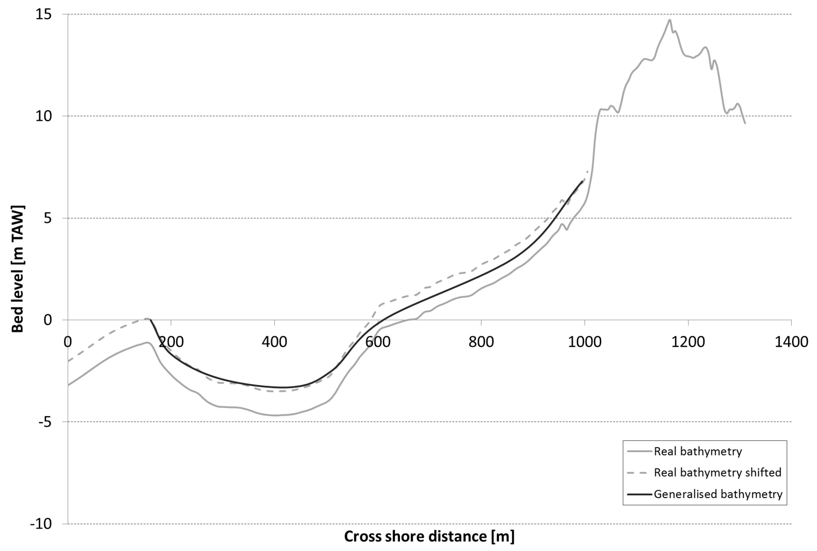
Figure 1 illustrates a typical post storm cross shore profile (grey line; black line indicates generalized profile, see further in §3.3). A sand bank creates an offshore bar with a crest at 1 m TAW. Landward of the bar the bed level decreases again to 4.5 m TAW , after which the foreshore has a slope of 1/88. Over a short distance closer to the dike , the slope steepens to 1/40 until the defined toe. This cross shore profile is shifted upward 1.2m to allow for more wave breaking at the bar and to end the foreshore at +6.8m TAW.

 Middenkust (coastal sections 61 to 195): The Middenkust covers the major part of residential coastal areas. Except for the small sandbank ‘stroombank’ off the city of Ostend, the near shore is gradually and uniformly changing from deeper water to the foreshore.

In addition, it is noted that not all coastal sections within a category correspond to the aforementioned typical cross shore profiles. It is however believed that the majority of coastal sections do fit (simplified) within the proposed categorisations.

For straightforward comparison between the wave overtopping results of SWASH and semi empirical equations, it is opted not to include the bended slope case in this project. Also emergent toe cases are not considered, nor foreshores including a/multiple berms and dikes including a storm wall.

Figure 3 illustrates a typical post storm cross shore profile (in case a storm is able to erode the beach until the dike) (grey line; black line indicates generalized profile, see further in §3.3). Landward of the gully, the 330 m wide foreshore has a slope of 1/50 until the dry part of the beach, where it steepens up to 1/20.

An important note to this categorisation is that the foreshore’s slope is rather uniformly mild alongshore while the slope’s transition to the ‘dry beach’ (roughly above 5 m TAW) depends on (i) whether or not beach nourishments are carried out (or dunes are located seaward of the dike) and (ii) if the beach erosion induced by the 45 hour lasting storm progressed on to the dike. Based on these varying conditions, a relatively uniform slope is found until the dike or a bended slope, consisting of a mild sloping foreshore which ends in a vertical cliff backed by a horizontal ‘dry beach’ (or dune) (see example in Figure 4).

10 WL2017R16_011_1 Final version

Figure 2 illustrates a typical post storm cross shore profile (in case a storm is able to erode the beach until the dike) (grey line; black line indicates generalized profile, see further in §3.3). The 1/50 foreshore uniformly continues to the dike where, over a short distance, it steepens up to 1/25 until the defined toe.

 Oostkust (coastal sections 232 to 248): Because of the nearby located Appelzak gully, the foreshore is rather short. However, its slope is comparably mild to the other categories, ending with a steeper short part closer to the dike.

Uncertainty in wave overtopping calculation using SWASH Shallow foreshore conditions (along the Flemish coast)

Uncertainty in wave overtopping calculation using SWASH Shallow foreshore conditions (along the Flemish coast) Final version WL2017R16_011_1 11 Figure 1 - General post storm bathymetry of the Westkust (Coastal section 25) Figure 2 - General post storm bathymetry of the Middenkust (Coastal section 103)

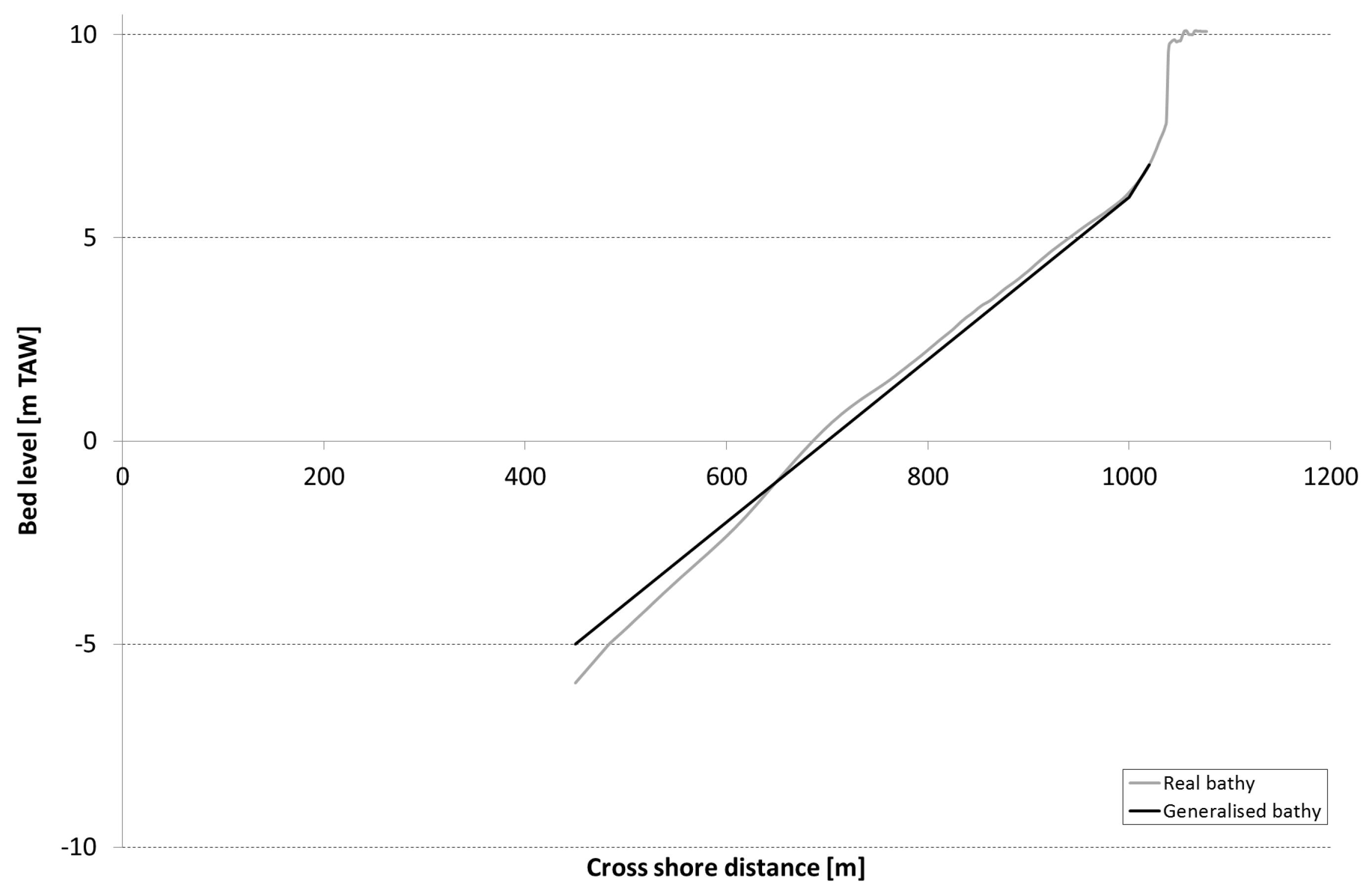
Uncertainty in wave overtopping calculation using SWASH Shallow foreshore conditions (along the Flemish coast) 12 WL2017R16_011_1 Final version Figure 3 - General post storm bathymetry of the Oostkust (Coastal section 233) Figure 4 - Coastal section 115: a beach nourishment is carried out, which stops storm induced erosion at a certain distance from the dike (Durosta calculation, Ruiz Parrado et al., 2016)

The first number ‘1XX’ indicates the use of SWASH 1D; hence, ‘2XX’ will be applied for wave transformation results of SWASH 2D. Schematisation

Table 1

Therespectively.Westkust generalized bathymetry, i.e. case 16X, starts at an offshore bar around 0 m TAW, i.e. around the mean low tide, where wave breaking might occur during storm events. This sandbar is located 865 m seaward of the toe of the dike Landward of the sandbar, a trough extends over 430m, reaching a maximum depth of 3.3 m TAW. Subsequently, a mild foreshore slope of 1/100 extends over 310 m after which it steepens to 1/35 over 125 m, until the toe of the dike.

The dike configuration is identical for all generalized bathymetries. It has a slope of ½ and a crest located at 3 different levels, i.e. +8.2 m TAW, +8.6 m TAW and +9 m TAW, in order to account for different quantities of wave overtopping. These levels correspond to case numbering XX3, XX2 and XX1 respectively.

The categorized bathymetries are further schematized into 6 generalisations, of which an overview is given in Table 1 and Figure 5 All generalized bathymetries are, according to Suzuki et al., 2016, artificially extended until 15m TAW following a 1/35 slope, followed by a horizontal stretch of 100 m Cases 10X, 14X and 16X are indicated (until the toe of the dike) by a black line in Figure 2, Figure 3 and Figure 1 respectively. Cases 11X and 13X, and case 15X are variations on case 10X and case 14X

Uncertainty in wave overtopping calculation using SWASH Shallow foreshore conditions (along the Flemish coast) Final version WL2017R16_011_1 13 3.3 Generalization of categorized bathymetries

The Middenkust generalized bathymetry includes a uniform foreshore slope of 1/50 until the toe of the dike for cases 11X and 13X whereas this slope contains a short steeper part of 1/25 close to the dike for case 10X. The foreshore is initiated 570 m seaward of the toe of the dike; in case 10X the steeper part takes up the last 20m before the toe of the dike.

The Oostkust generalized bathymetry, i.e. cases 14X and 15X, has a uniform foreshore slope of 1/50 (identical to the Middenkust bathymetry). In case 14X, this slope includes a short steeper part of 1/20 close to the dike. The foreshore starts at 285 m seaward of the toe of the dike, i.e. at half the distance of the Middenkust foreshore. Case 14X is 40 m longer, accounting for the short steeper part.

of the categorized bathymetries 10X 11X 13X 14X 15X 16X foreshoreLength [m] 570 570 570 325 285 865 foreshoreSlope [ ] 1/501/25 1/50 1/50 1/501/20 1/50 1/1001/35 Level foreshorestart [m TAW] 5 5 4.6 0.9 1.1 0 Toe level [m TAW] 6.8 6.4 6.8 6.8 6.8 6.8 Crest level [m TAW] +9 (X = 1) +8.6 (X = 2) +8.2 (X = 3)

Uncertainty in wave overtopping calculation using SWASH Shallow foreshore conditions (along the Flemish coast) 14 WL2017R16_011_1 Final version Figure 5 - Generalized post storm bathymetries

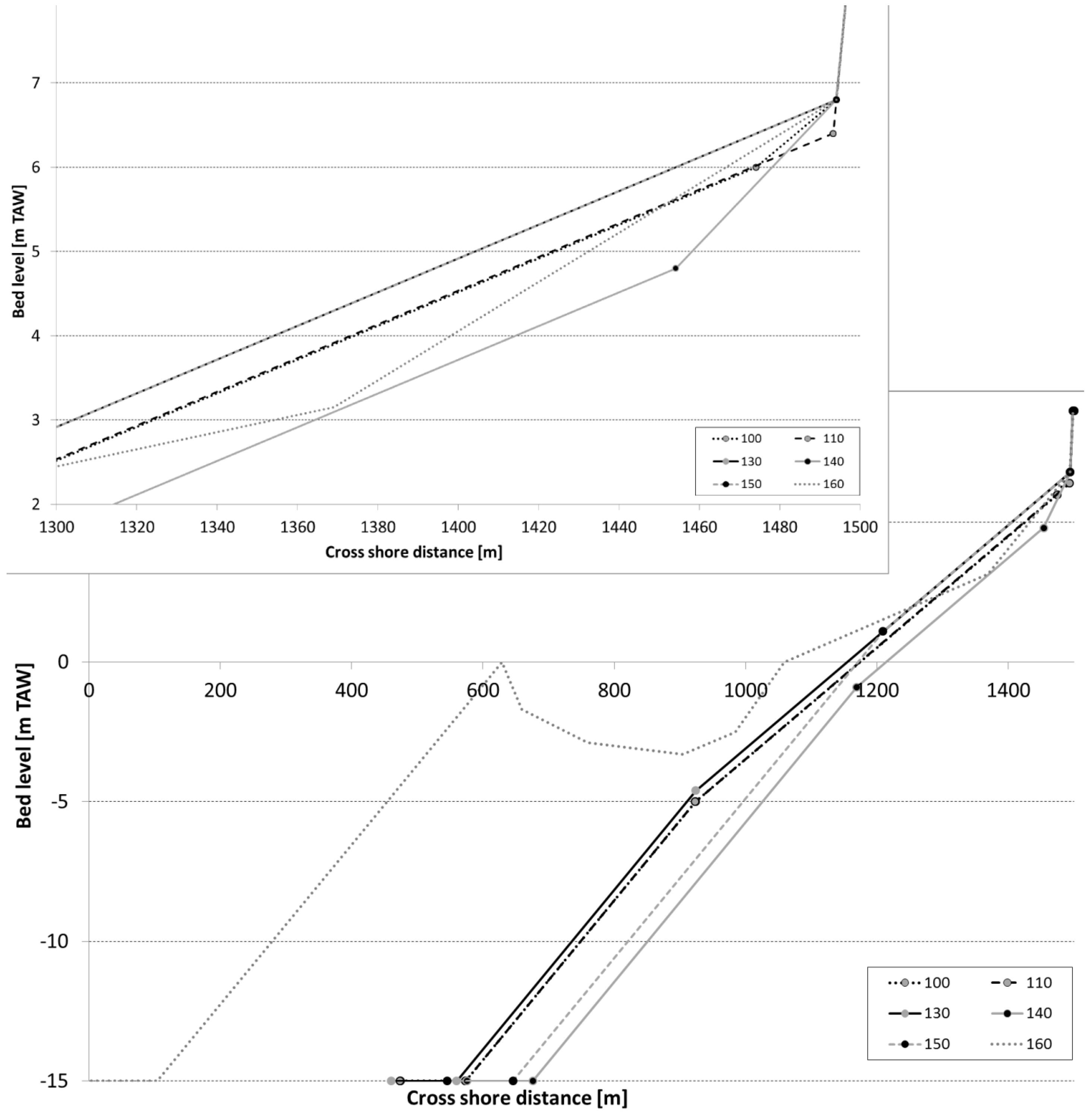
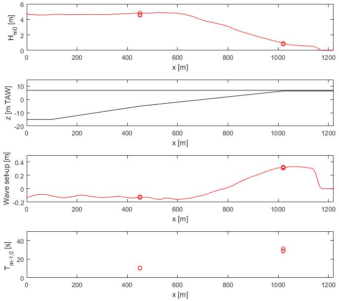
Figure 9, Figure 10, Figure 11, Figure 12, Figure 13 and Figure 14 illustrate the wave parameters and spectra at 5m TAW and at the toe of the dike for the randomly chosen seed number 12345140 given case 200, 210, 230, 240, 250 and 260 respectively.

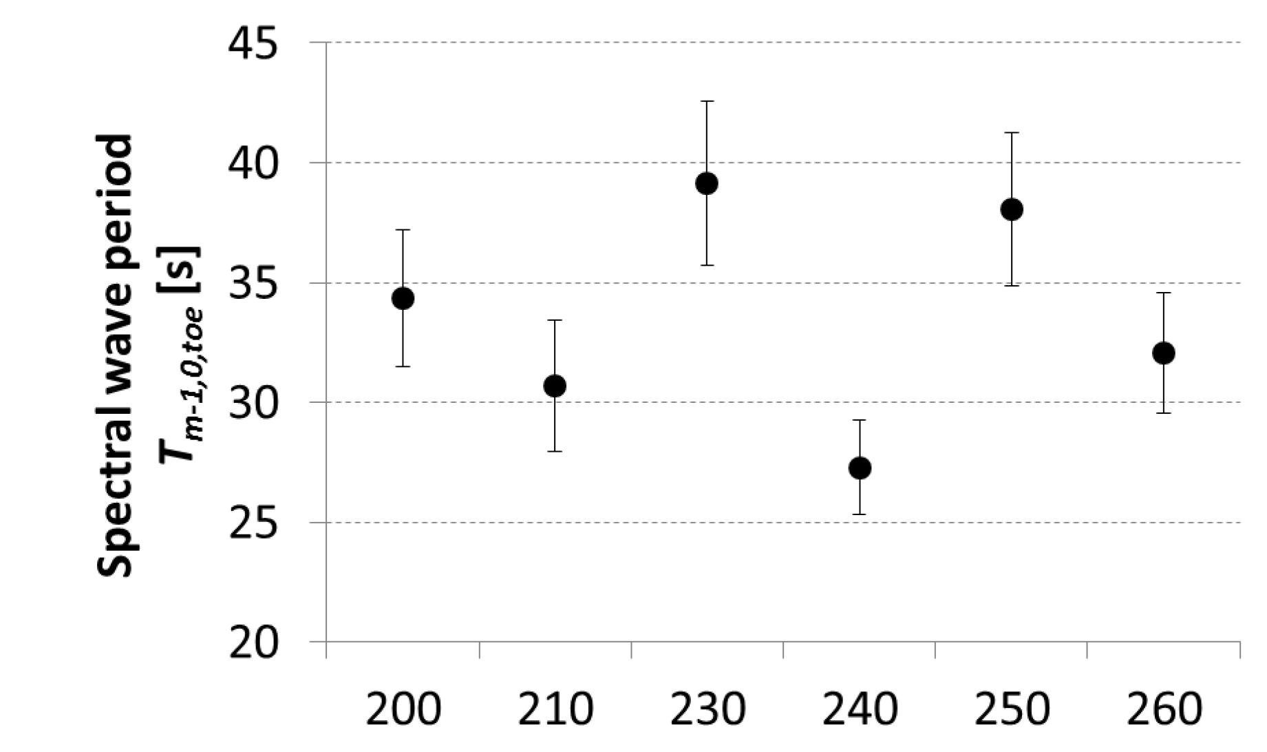
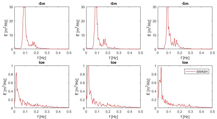
The higher the significant wave height Hm0 at the toe of the dike, the lower its associated spectral wave period Tm 1,0. Significant wave heights Hm0 are highest for case 240, followed by case 210 (having a larger water depth at the toe) and cases 200 and 260. Cases 230 and 250 have the lowest significant wave heights Hm0. Looking at the respective wave spectra at 5m TAW and at the toe, the energy transfer from short waves (>0.05 Hz = < 20s) to infragravity waves is clearly visible for all cases. The greatest part of the remaining wave energy is within their frequency band, having a peak frequency around 0.18Hz.

Final version WL2017R16_011_1 15 4 SWASH model train 4.1

Figure 6, Figure 7 and Figure 8 indicate the mean significant wave height Hm0, spectral wave period Tm 1,0 and wave set up at the toe of the dike respectively for all cases.

Uncertainty in wave overtopping calculation using SWASH Shallow foreshore conditions (along the Flemish coast) 2D wave transformation 4.1.1 Setup Table 2 lists the hydraulic boundary conditions used as input to SWASH 2D for the wave transformation from offshore until the toe of the dike. They correspond with a 1000 year return period and are located at specific 5m TAW coordinates in coastal section 105 (Oostende Raversijde). The water level is fixed; wave conditions are applied as a JONSWAP spectrum with a peak enhancement factor of 3.3 and a (one sided) directional spreading of 16°. The simulated wave train consisted of at least 200 waves. This hydraulic input was identical for the 6 generalized bathymetry cases (cf. Table 1). These bathymetries were implemented in quasi 2D, i.e. the cross shore profiles were uniformly extended alongshore over a distance of 400 m, without dike configuration.

Table 2 Offshore hydraulic boundary conditions (RT= 1000 year, CS 105 in De Roo et al., 2016) Water level SWL [m TAW] Significant wave height Hm0 [m] Peak wave period Tp [s] Directional spreading σ [°] 6.9 4.6 11.3 16 4.1.2 Results: incident hydraulic boundary conditions at the toe of the dike

SWASH simulations were carried out according to the methodology described in Appendix A of Suzuki et al., 2016. For every case, the seed number was varied 300 times, from 12345001 till 12345300.

16 Final version

Figure 6 - Mean incident significant wave height Hm0 at the toe of the dike. Error bars indicate the standard deviation (n = 300 except for 260: n = 291)

Uncertainty wave overtopping calculation using SWASH Shallow foreshore conditions (along the Flemish coast)

Figure 7 - Mean spectral wave period Tm-1,0 at the toe of the dike. Error bars indicate the standard deviation (n = 300 except for 260: n = 291)

WL2017R16_011_1

Cases 230 and 250, having a uniform mild foreshore slope of 1/50, result in a relatively low significant wave height Hm0 and both high spectral wave period Tm-1,0 and wave set up compared to cases 200 and 240, having a short steeper part close to the toe. The shorter surf zone of case 250, having a foreshore half the length of case 230, results in a faster wave breaking and increase in wave set up, leading to a slightly smaller contribution of the infragravity waves to the spectral wave period Tm-1,0. The short steeper part of the foreshore close to the toe of the dike in case 200 (240) leads to a different wave transformation compared to case 230 (250). Its relative influence is higher the shorter the foreshore’s length is.

version WL2017R16_011_1 17

Uncertainty in wave overtopping calculation using SWASH Shallow foreshore conditions (along the Flemish coast)

Waves feel this transition and steepen, which results in a higher significant wave height Hm0, lower wave set-up and lower spectral wave period Tm-1,0. This is indicated in the wave spectra seeing the relatively higher short wave contribution.

Final Figure 8 - Mean wave set up at the toe of the dike. Error bars indicate the standard deviation (n = 300 except for 260: n = 291)

Consequently, it seems that the length of the foreshore, having a slope of 1/50, is less important than the steepness of its slope close to the dike, seeing that cases 230 (length = 570m) and 250 (length = 285m) lead to similar incident wave conditions and the results of cases 200 and 240 are clearly different from these Case 210, having a larger water depth (0.80 m compared to 0.48 m (case 230)), experiences accordingly less wave breaking and hence, a larger significant wave height Hm0 and both lower spectral wave period Tm-1,0 and wave set up. Case 260, having a longer (yet different) bathymetry compared to the other cases, results in comparable incident hydraulic boundary conditions. Some wave breaking occurs at the offshore bar and later on the foreshore after the trough, being enhanced at the end on the steeper part close to the toe of the dike After the bar and trough, this foreshore is somewhat shorter (435m) compared to case 230 (570m) and ends in a milder yet longer slope (1/35 – 125 m) close to the dike compared to 200 (1/25 -20m) and 240 (1/20 – 40m).

To conclude, both the water depth and the steepness of the foreshore’s slope close to the toe of the dike significantly affect the incident hydraulic boundary conditions. A smaller water depth and milder foreshore slope lead to a lower significant wave height Hm0 and higher spectral wave period Tm-1,0 and wave set up.

Uncertainty in wave overtopping calculation using SWASH Shallow foreshore conditions (along the Flemish coast) 18 WL2017R16_011_1 Final version Figure 9 Case 200I wave parameters and spectra at 5m TAW and toe of the dike (seed 12345140)

Uncertainty in wave overtopping calculation using SWASH Shallow foreshore conditions (along the Flemish coast) Final version WL2017R16_011_1 19 Figure 10 Case 210I wave parameters and spectra at 5m TAW and toe of the dike (seed 12345140)

Uncertainty in wave overtopping calculation using SWASH Shallow foreshore conditions (along the Flemish coast) 20 WL2017R16_011_1 Final version Figure 11 Case 230I wave parameters and spectra at 5m TAW and toe of the dike (seed 12345140)

Uncertainty in wave overtopping calculation using SWASH Shallow foreshore conditions (along the Flemish coast) Final version WL2017R16_011_1 21 Figure 12 Case 240I wave parameters and spectra at 5m TAW and toe of the dike (seed 12345140)

Uncertainty in wave overtopping calculation using SWASH Shallow foreshore conditions (along the Flemish coast) 22 WL2017R16_011_1 Final version Figure 13 Case 250I wave parameters and spectra at 5m TAW and toe of the dike (seed 12345140)

Uncertainty in wave overtopping calculation using SWASH Shallow foreshore conditions (along the Flemish coast) Final version WL2017R16_011_1 23 Figure 14 Case 260I wave parameters and spectra at 5m TAW and toe of the dike (seed 12345140)

SWASH simulations were carried out according to the methodology described in Appendix B of Suzuki et al., calibration setups were executed:

To carry out setup 2, a simple matlab routine was programmed to automate the calibration. After 9 loops, calibration was stopped if no matching criteria were obtained. Table 5 lists the success rate. The success rate of case 160 is remarkably lower because of time restrictions to finetune the calibration routine.

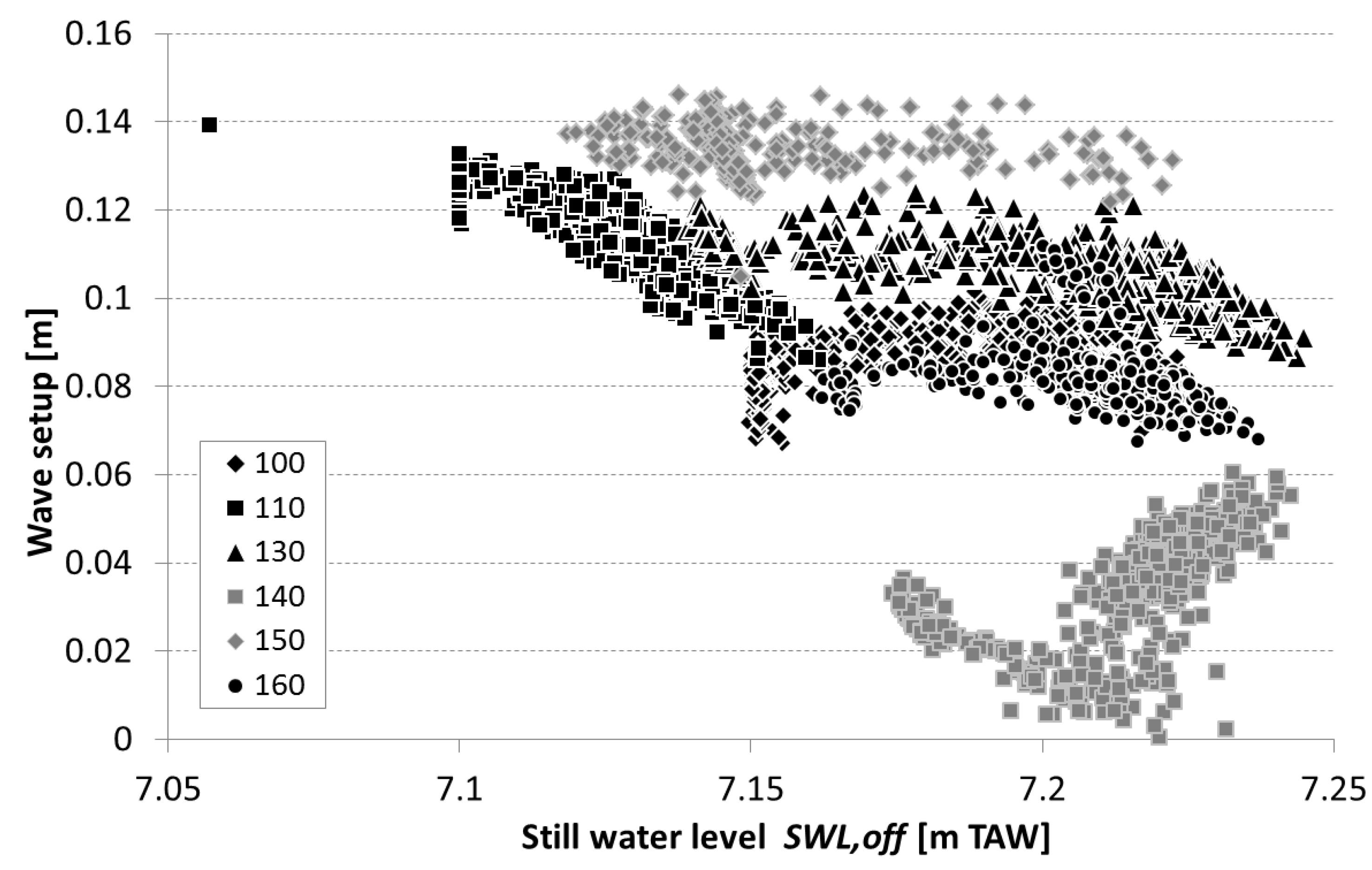
Figure 15 and Figure 16 depict the calibrated offshore significant wave height Hm0,off and still water level SWL respectively. Both variables might differ considerably between the selected seed numbers. In general, the difference in significant wave height Hm0 between seed numbers varies more than the difference in still water level SWL. Comparing the seed dependent and one seed calibration results to the 2D input conditions, it is clear that the significant wave heights Hm0 are significantly lower than the 2D value (4.6 m), taking as a rough estimate half of that value. The still water level SWL is somewhat higher than +6.9 m TAW, i.e. 0.1 to 0.3 m case Comparingdependent.the calibration setups with each other, seed dependent significant wave heights Hm0 are higher, i.e. 0.2 to 0.5 m case dependent, whereas still water levels SWL are alike except for one seed calibrated cases 100 and 160 having a 0.05 m higher still water level (cf. Figure 16).

The calibration purpose is to obtain matching incident hydraulic boundary conditions at the toe of the dike using SWASH 1D. By altering iteratively the offshore boundary conditions of water level and significant wave height, it is tried to achieve similar incident hydraulic boundary conditions to the average SWASH 2D results, i.e. within the calibration limits (Table 3) The simulated wave train consisted of at least 500 waves.

Two2016different

Table 3 Calibration criteria to be met concurrently for the incident hydraulic boundary conditions at the toe of the dike Water level SWL + wave set up Significant wave height Hm0 Spectral wave period Tm 1,0 ±0.05 m ± 3% ± 5% 4.2.2 Results: calibration Setup 1, carried out in the first phase of the project, was executed by simulating a matrix of possible input boundary conditions. Then, one pair out of all matching conditions was selected (Table 4, column 2 and 3).

1. For every case, the seed number was varied 500 times, from 12345001 till 12345500. Only seed number 12345001 was calibrated to match the average 2D results, and these results were applied to all seed numbers’ simulations 2. For every case, the seed number was varied 500 times, from 12345001 till 12345500. Every seed number was calibrated to match the average 2D results.

Uncertainty in wave overtopping calculation using SWASH Shallow foreshore conditions (along the Flemish coast) 24 WL2017R16_011_1 Final version 4.2 1D calibration of wave transformation 4.2.1 Setup

Uncertainty in wave overtopping calculation using SWASH Shallow foreshore conditions (along the Flemish coast) Final version WL2017R16_011_1 25 Table 4 Results for setup 1: calibration of seed 12345001 OFFSHORE TOE Case Still water level [m TAW] waveSignificantheight Hm0 [m] Water level [m TAW] SWL + wave set up Significantheightwave Hm0 [m] Spectralperiodwave Tm 1,0 [s] 100 7.20 2.0 7.20 + 0.06 0.78 34.8 110 7.16 1.8 7.16 + 0.09 0.81 30.9 130 7.20 1.9 7.20 + 0.11 0.67 39.4 140 7.22 2.0 7.22 + 0.04 0.86 27.0 150 7.20 2.3 7.20 + 0.13 0.67 38.9 160 7.24 1.3 7.24 +0.07 0.73 32.6 Table 5 Success rate for setup 2: calibration of 500 individual seed numbers Case # calibrations matched? 100 500 110 475 130 478 140 481 150 496 160 385

Uncertainty in wave overtopping calculation using SWASH Shallow foreshore conditions (along the Flemish coast) 26 WL2017R16_011_1 Final version Figure 15 - Seed dependent calibration of the significant wave height Hm0,off

Given the same offshore significant wave height Hm0,off, wave set-up decreases when the still water level SWL increases because of less wave breaking. It is proportional to the offshore significant wave height Hm0,off A higher wave set up does not always result from a higher offshore significant wave height Hm0,off because the calibrated still water level SWL varies given a certain wave height.

4.2.3 Results: incident hydraulic boundary conditions at the toe of the dike

Uncertainty in wave overtopping calculation using SWASH Shallow foreshore conditions (along the Flemish coast) Figure 16 - Seed dependent calibration of the still water level SWLoff

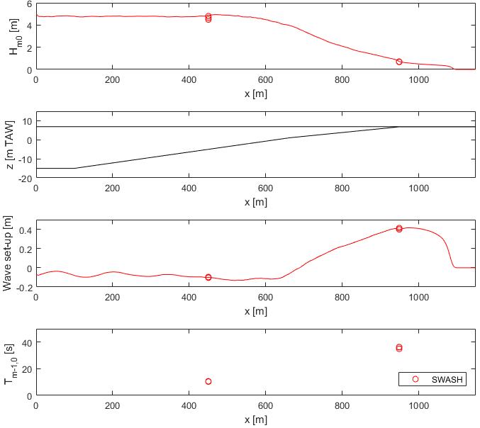
Table 4 lists the results of setup 1. Figure 17, Figure 18 and Figure 19 respectively illustrate the setup 2 results of wave set up, significant wave height Hm0 and spectral wave period Tm-1,0 Figure 20, Figure 21, Figure 22, Figure 23, Figure 24 and Figure 25 show the wave parameters and spectra at 5m TAW and at the toe of the dike for the selected ‘perfectly calibrated’ seed numbers of setup 2 (perfect calibration, see further in 6.1) given case 100, 110, 130, 140, 150 and 160 respectively.

Final version WL2017R16_011_1 27

The biggest difference between SWASH in 2D and 1D mode is the resulting water level and associated wave set-up at the toe of the dike: a lower still water level SWL and higher wave set up are measured in 2D compared to 1D. This leads to a different start of the surf zone in 1D, i.e. closer to the toe of the dike, and hence, a shorter region of wave breaking and wave set up. Yet, the respective wave spectra at the toe of the dike are similar to the 2D spectra.

Besides the shorter surf zone in 1D, wave transformation of case 160 and 260 differ. The higher still water level SWL and lower significant wave height offshore Hm0,off result in a very short zone of wave breaking in 1D, starting at about 1400m cross shore distance (at transition to 1/35 slope) instead of 600m (at the offshore bar) The wave spectra at the toe of the 2D and 1D cases are however alike

Figure 26, Figure 27 and Figure 28 respectively depict the differences in mean significant wave height Hm0, spectral wave period Tm 1,0 and wave set up at the toe of the dike applying calibration setup 1 ‘one seed’ and 2 ‘all seeds’ for all cases Regarding the former setup, 500 simulations were carried out using the calibrated offshore boundary conditions of seed number 12345001 whereas the latter setup includes the results of seed dependent calibrated boundary conditions.

In general, mean incident hydraulic boundary conditions are somewhat lower for the ‘one seed’ setup compared to the ‘all seeds’ setup. In comparison to the incident 2D results, the ‘one seed’ setup results are up to 8% lower for significant wave height Hm0, varying between 25% and +15% for spectral wave period Tm 1,0 and range within the calibration limits (±0.05m, cf. Table 3) for wave set up. The ‘one seed’ wave parameters’ standard deviation is similar to the ‘all seeds’ setup for significant wave height Hm0 and wider for spectral wave period Tm 1,0. Conversely, the ‘all seeds’ wave set up varies more because of the varying offshore significant wave heights and still water levels

Note that, given a certain seed, various offshore parameter combinations might lead to a (calibration) match with the 2D reference values at the toe of the dike. A different parameter combination possibly leads to another wave overtopping discharge

Uncertainty in wave overtopping calculation using SWASH Shallow foreshore conditions (along the Flemish coast)

Final version Wave set up is highest for cases 150 and 130, being in accordance with the 2D results, and case 110. The latter case, having the lowest wave set up in 2D (0.3 m, see Figure 8), now has comparatively a larger wave set up in 1D because the magnitude of its wave set up in 2D is partly compensated by the magnitude of the calibrated still water level SWL in 1D. In absolute value however, it logically is lower (0.11, see Figure 17).

28 WL2017R16_011_1

Uncertainty in wave overtopping calculation using SWASH Shallow foreshore conditions (along the Flemish coast) Final version WL2017R16_011_1 29 Figure 17 - Seed dependent wave set up in relation to the offshore significant wave height Hm0,off Figure 18 - Seed dependent wave set up in relation to the offshore still water level SWLoff

Uncertainty in wave overtopping calculation using SWASH Shallow foreshore conditions (along the Flemish coast) 30 WL2017R16_011_1 Final version Figure 19 - Seed dependent significant wave height Hm0,toe and associated spectral wave period Tm-1,0,toe at the toe of the dike

Uncertainty in wave overtopping calculation using SWASH Shallow foreshore conditions (along the Flemish coast) Final version WL2017R16_011_1 31 Figure 20 Case 100I wave parameters and spectra at 5m TAW and toe of the dike (seed 12345261)

Uncertainty in wave overtopping calculation using SWASH Shallow foreshore conditions (along the Flemish coast) 32 WL2017R16_011_1 Final version Figure 21 Case 110I wave parameters and spectra at 5m TAW and toe of the dike (seed 12345146)

Uncertainty in wave overtopping calculation using SWASH Shallow foreshore conditions (along the Flemish coast) Final version WL2017R16_011_1 33 Figure 22 Case 130I wave parameters and spectra at 5m TAW and toe of the dike (seed 12345470)

Uncertainty in wave overtopping calculation using SWASH Shallow foreshore conditions (along the Flemish coast) 34 WL2017R16_011_1 Final version Figure 23 Case 140I wave parameters and spectra at 5m TAW and toe of the dike (seed 12345451)

Uncertainty in wave overtopping calculation using SWASH Shallow foreshore conditions (along the Flemish coast) Final version WL2017R16_011_1 35 Figure 24 Case 150I wave parameters and spectra at 5m TAW and toe of the dike (seed 12345079)

Uncertainty in wave overtopping calculation using SWASH Shallow foreshore conditions (along the Flemish coast) 36 WL2017R16_011_1 Final version Figure 25 Case 160I wave parameters and spectra at 5m TAW and toe of the dike (seed 12345434)

Error bars indicate the standard deviation (one seed: n = 500; all seeds: n cf. Table 5)

Figure 26 Mean incident significant wave height Hm0 at the toe of the dike for the 2 calibration setups

Figure 27 Mean spectral wave period Tm 1,0 at the toe of the dike for the 2 calibration setups

Uncertainty in wave overtopping calculation using SWASH Shallow foreshore conditions (along the Flemish coast)

Final version WL2017R16_011_1 37

Error bars indicate the standard deviation (one seed: n = 500; all seeds: n cf. Table 5)

4.3 1D wave overtopping

SWASH sometimes experiences numerical instability. In order to reduce the number of instabilities, time integration was explicitly set between 0.1 and 0.5 (based on the Courant number). If the maximum of the Courant number over all wet grid points is higher than the pre set maximum, the time step is halved On the contrary, if it is lower than the pre set minimum, the time step is doubled.

Following calibration setup 1, the offshore input (Hm0, SWL) is identical for the 500 SWASH simulations, in which the seed number was varied 500 times, from 12345001 till 12345500. Following calibration setup 2, the offshore input is seed dependent.

Uncertainty in wave overtopping calculation using SWASH Shallow foreshore conditions (along the Flemish coast) 38 WL2017R16_011_1 Final version Figure 28 Mean wave set up at the toe of the dike for the 2 calibration setups Error bars indicate the standard deviation (one seed: n = 500; all seeds: n cf. Table 5)

4.3.2 Numerical instability

Table 6 summarizes the number of simulations that stopped too early and hence, did not produce a wave overtopping result. Note that the number of simulations included in the analysis is lower than this number of instable simulations since it also depends on the success rate of the seed dependent calibration (cf. Table 5)

4.3.1 Setup Using the results of calibration setup 1 and 2, wave overtopping is calculated with SWASH 1D for 3 dike configurations (different crest level, cf. Table 1) per case. For every dike configuration, 500 SWASH simulations were carried out, in which the wave train consisted of at least 500 waves. These simulations were carried out according to the methodology described in Appendix B of Suzuki et al., 2016.

Uncertainty in wave overtopping calculation using SWASH Shallow foreshore conditions (along the Flemish coast) Final version WL2017R16_011_1 39 Table 6 Number of instable wave overtopping simulations using one seed calibration (between brackets) and seed dependent calibration input values Case Crest level X = 1 X = 2 X = 3 10X (80) 77 (63) 50 (50) 43 11X (130) 61 (165) 84 (134) 55 13X (40) 30 (129) 28 (117) 20 14X (228) 75 (219) 48 (231) 42 15X (99) 40 (120) 41 (112) 27 16X (51) 39 (44) 51 (19) 30

A larger water depth at the toe, resulting in higher waves, has less influence on the amount of wave overtopping compared to a short steeper foreshore part close to the toe, given the smaller wave overtopping for case 111 compared to 101 (131 being the reference case). Still, given an identical bathymetry, a larger water depth does lead to higher wave overtopping (case 111 compared to 131). These findings hold for all freeboards. Depending on the bathymetric configuration, the variability in wave overtopping differs (given the different boxplot sizes).

Uncertainty in wave overtopping calculation using SWASH Shallow foreshore conditions (along the Flemish coast) 40 WL2017R16_011_1 Final version 4.3.3

The standard deviation’s magnitude is dependent on the wave overtopping’s magnitude and the population size; hence, it is higher in absolute terms for higher wave overtopping discharges and smaller population size Figure 31 (zoom in Figure 32) and Figure 33 (zoom in Figure 34) depict the boxplots of the wave overtopping data for every dike configuration in all cases given the one seed and seed dependent calibration setup respectively. The bottom and top of the box indicate the first and third quartile of the data respectively, in which the second quartile, i.e. the median, is shown; hence, the midspread, or middle 50%, of the data is included in the box. The whiskers point out the limits of 1.5 times the interquartile range. Some populations include outliers, i.e. points located outside the whiskers.

Results: wave overtopping Figure 29 (zoom in Figure 30) shows the mean wave overtopping discharge and its standard deviation for every dike configuration in all cases using the 2 calibration setups, which slightly differ from one another. Yet, this mean and corresponding standard deviation do have another origin. Identical offshore boundary conditions, i.e. setup 1, account purely for the random nature of waves in their transformation and result in (possibly) different conditions at the toe of the dike. On the contrary, (possibly) different offshore boundary conditions, i.e. setup 2, result in identical conditions at the toe of the dike (within calibration limits). The associated wave overtopping discharge depends on these conditions at the toe of the dike and on the wave transformation characteristics of the considered surface elevation time series.

The higher the crest of the dike, the higher its freeboard and hence, the lower the wave overtopping over it. Cases 101, 111, 131, 141, 151 and 161 therefore show the smallest amount of wave overtopping, which exponentially increases with lowering the crest level in cases XX2 and XX3 respectively

Given the crest of the dike at 9 m TAW, case 141 significantly results in the highest wave overtopping because it has the highest waves at the toe (irrespective of a smaller infragravity wave influence). Cases 101 and 161 result in comparable wave overtopping discharges. Their longer foreshore, compared to 141, leads to a larger infragravity wave influence. It ends in a short steeper part close to the toe, facilitating and hence, increasing wave overtopping compared to case 131. These findings logically hold for the other freeboards too.

Uncertainty in wave overtopping calculation using SWASH Shallow foreshore conditions (along the Flemish coast) Final version WL2017R16_011_1 41 Figure 29 - Mean wave overtopping discharge (error bars indicate the standard deviation). Figure 30 - Zoom on mean wave overtopping discharge (excluding case 143) (error bars indicate the standard deviation).

Uncertainty in wave overtopping calculation using SWASH Shallow foreshore conditions (along the Flemish coast) 42 WL2017R16_011_1 Final version Figure 31 Boxplots of wave overtopping discharge q (one seed calibration) Figure 32 Zoom on boxplots of wave overtopping discharge q (excluding case 143; one seed calibration)

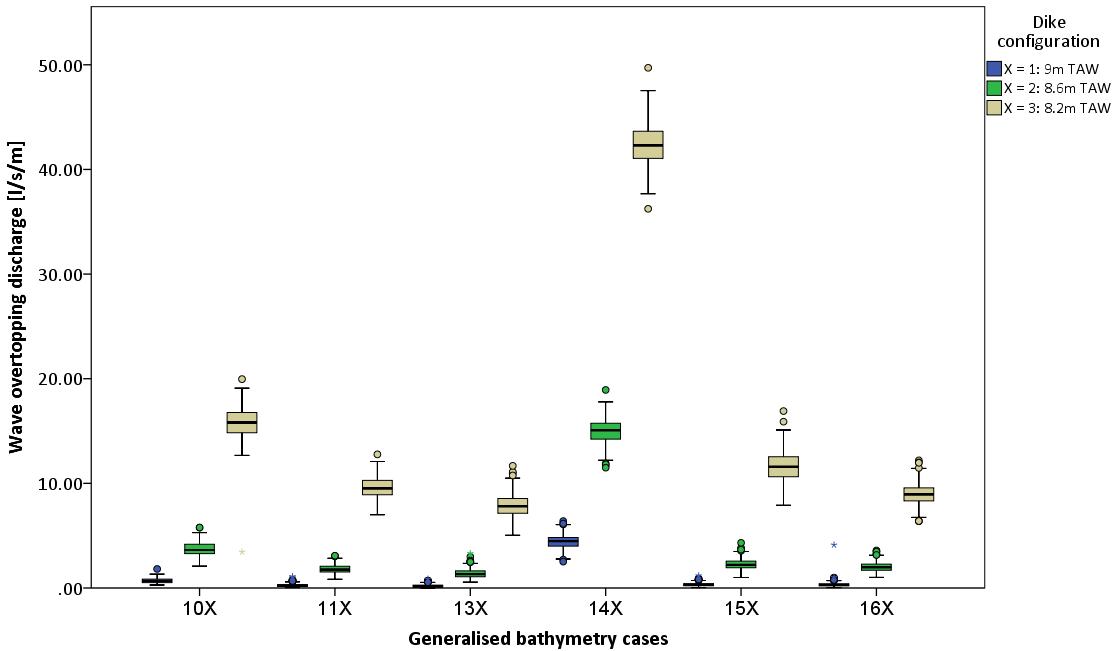
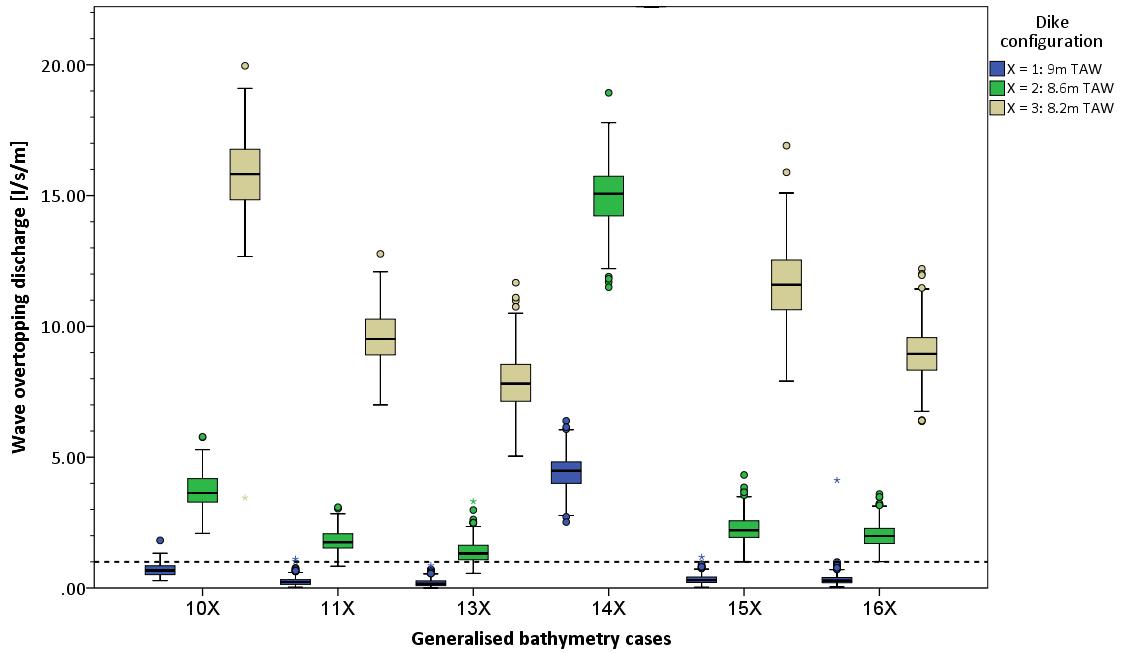
Uncertainty in wave overtopping calculation using SWASH Shallow foreshore conditions (along the Flemish coast) Final version WL2017R16_011_1 43 Figure 33 Boxplots of wave overtopping discharge q (seed dependent calibration) Figure 34 Zoom on boxplots of wave overtopping discharge q (excluding case 143; seed dependent calibration)

Uncertainty in wave overtopping calculation using SWASH Shallow foreshore conditions (along the Flemish coast) 44 WL2017R16_011_1 Final version 4.3.4

The underlying statistical distribution of the wave overtopping results is investigated for the seed dependent results. It is evaluated whether or not the data follow a (log)normal distribution, being the common distribution for wave overtopping data (cf. Section 2.2). Both the Kolmogorov Smirnov and Shapiro Wilk tests are applied, and the Normal Q Q plot is checked. Appendix 2 lists the results.

The assumption of normality for these wave overtopping populations implies that not a unique value is describing the data but a range of possible values, which are described by the mean µ, being the expected value of the data, and the standard deviation σ, indicating the spread of these data around the mean. The uncertainty on this wave overtopping population can be quantified in terms of relative error, being a coefficient of variation: �� ′ = �� (12)

Basedhypotheses.onthese

The data of cases 102, 103, 112, 141, 142 and 143 is normally distributed (the null hypothesis is accepted).

Results: statistical distribution of wave overtopping data

In general, the lower the mean wave overtopping discharge, the more outliers are observed at higher values and hence, the more the distribution became positively skewed. Contrary, the higher the mean wave overtopping discharge, the more symmetrical the distributions became.

The data of cases 132, 133, 152, 153, 161 and 162 follows a lognormal distribution, i.e. the natural logarithm of these variables is normally distributed. Lognormal transformation often occurs when the 95.5% range of a normal distribution, i.e. µ±2σ, extends below 0, being physically impossible. It reduces this positive skewness of the data. Nonetheless, cases 101, 111, 113, 131, 151 and 163 reject both null

findings and relying on the central limit theorem, i.e. a distribution of �� tends towards a normal distribution even when Y is not normally distributed on condition that the number of observations n is large (n > 60), a normal distribution is assumed for all wave overtopping populations

Final version WL2017R16_011_1 45 5 Wave

5.1 Influence of boundary conditions

The freeboard combines the influence of the water level and the crest level of the structure. Figure 37 shows the wave overtopping discharge in relation to this freeboard, both parameters being dimensionless based on the incident significant wave height Hm0. Logically, the higher the freeboard, the less wave overtopping occurs (exponential relation). On the contrary, the variability in wave overtopping increases with the freeboard because the probability that a wave, or several waves, overtop highly depends on the individual wave characteristics in the time series.

Uncertainty in wave overtopping calculation using SWASH Shallow foreshore conditions (along the Flemish coast) overtopping

Because of the importance of having a matching calibration for every seed number, mean wave overtopping discharges are, as from this Chapter, only discussed for setup 2: seed dependent calibration

Wave overtopping is determined by (i) the incident hydraulic boundary conditions, i.e. the significant wave height, the spectral wave period and the water level, at the toe of the structure and (ii) the characteristics of the foreshore and structure (e.g. the crest level, the slopes of the foreshore and structure, the presence of a berm...)

The influence of the foreshore on the incident wave conditions at the toe of the dike is reflected in the very low wave steepness sm 1,0 (Figure 35). It ranges from 0.2∙10 3 till 0.8∙10 3, for all cases being lower than 0.005, the limit indicating whether or not a shallow foreshore is present (Altomare et al., 2016) It is highest for case 140, having a short foreshore and steeper part, which leads to the largest wave heights and lowest wave periods (cf. Figure 19). Furthermore, the ratio between the water depth and incident wave height, which is always smaller than 1.5, also indicates the very shallow water conditions (Figure 36).

For the highest relative freeboards, wave overtopping might vary up to a factor 100 or 200, given cases 151O and 131O respectively (crest level at +9m TAW). For the lowest relative freeboards, wave overtopping varies only a factor 1.7 or 2.3, given cases 143O and 163O (crest level at +8.2m TAW).

Uncertainty in wave overtopping calculation using SWASH Shallow foreshore conditions (along the Flemish coast) 46 WL2017R16_011_1 Final version Figure 35 - Wave steepness sm-1,0 for all cases Figure 36 - Ratio between the water depth dtoe and incident wave height Hm0,toe at the toe of the dike for all cases

Uncertainty in wave overtopping calculation using SWASH Shallow foreshore conditions (along the Flemish coast) Figure - Dimensionless wave overtopping discharge Qdim in relation to the relative freeboard Rc*

The scope of the project entails shallow foreshore conditions, which now are confirmed by the results of wave steepness sm-1,0 and the ratio between the water depth and wave height at the toe dtoe/Hm0,toe. Hence, the proposed equation 1 (including the coefficients of equation 5 or 6) is to be applied in comparison with the SWASH results, using the incident hydraulic boundary conditions calibrated in SWASH 1D (Figure 15 and Figure Besides16).the relative freeboard R* (cf Figure 37), the surf similarity parameter ��−1,0 is the other variable to be introduced in the wave overtopping equations. Combining the wave steepness sm-1,0 and the equivalent slope, a breaker parameter ��−1,0 ranging from 4.6 to 8.1 is obtained for all cases. The average slope 1/m is calculated using equation 3 and ranges from 5.5 to 11.5 (cf Figure 38).

Final version WL2017R16_011_1 47

5.2 Results: SWASH vs. empirical equations

Uncertainty in wave overtopping calculation using SWASH Shallow foreshore conditions (along the Flemish coast) WL2017R16_011_1 Figure 39 and Figure 40 show the wave overtopping results (dimensionless) of SWASH compared to empirical equations. The latter are used in a probabilistic way, i.e. applying the mean value of equation 5 (‘Qdim MB’) or 6 (‘Qdim Alto’) in the coefficient 10�� of equation 1. The similarity between the model and empirical results deteriorates the smaller the wave overtopping discharges become, where the model results are increasingly smaller than the empirical results. Given that the coefficient cQ in equation 5 is lower than in equation 6, the former equation provides a slightly better agreement with the model results

Logically, the same tendency visible in Figure 39 and Figure 40 is noticed here: the smaller the wave overtopping discharge, the smaller the ratio QSWASH/ Qeq,MB,det, the higher the divergence between both results. The majority of the SWASH results leads to a ratio between 0.1 to 0.8, indicating a mismatch between both methods of up to one order of magnitude. Yet, cases 142O, 143O and 153O, leading to high wave overtopping discharges, well agree with the equation.

However, one should keep in mind the findings of Altomare et al. (2016) regarding that equation (see Section 2.2) For dimensionless wave overtopping discharges higher than 4, the results are quite comparable. The SWASH results are contained within 0.5 to 2 times the empirical results for all cases ‘XX3’, which correspond to a crest level of the dike at +8.2 m TAW including case 142 too and have a relative freeboard R* lower than 1.6. In the wave overtopping interval between 1 (1.5 for ‘Qdim Alto’) and 4, corresponding to a relative freeboard R* between 1.6 and 2.2, the SWASH results are up to one order of magnitude smaller.

Final version

The biggest differences are noted for cases 101, 132 and 112 compared to the closer matching cases 141, 152, 162 and 102. Below a dimensionless wave overtopping discharge of 1 (1.5), the SWASH results significantly differ from the empirical ones, having the highest divergence for cases 131 and 111 whereas cases 151 and 161 correspond better to the equation.

Furthermore, it seems that cases 10X, 11X and 13X, having the longest uniform foreshore slope (of 1/50), deviate the most, being most pronounced for higher freeboards. They include the longest surf zone, where wave breaking and wave set up take place; hence, this local increase of the water level might facilitate waves overtopping the structure. Although wave set up is implicitly reproduced in the physical model tests (over a scale dependent foreshore length), its influence should additionally accounted for when the foreshore is very long and gently according to Allsop et al., 2016. Besides, long wave energy cannot be absorbed in a wave flume. When a (very) shallow foreshore condition is modelled, infragravity wave energy will accumulate leading to an increased wave overtopping discharge. The two phenomena have an opposite effect on the measured wave overtopping discharge; yet, it seems that the latter one is most pronounced.

The higher the freeboard, the lower the number of waves that overtop, the more important these individual wave’s overtopping characteristics become (cf. Section 2.1 and 2.2). Consequently, the more the wave overtopping results of SWASH and equation diverge because the latter does not account for this uncertainty, or more precise variability, in mean wave overtopping discharge.

In the safety assessment, the wave overtopping discharge is calculated with SWASH and equation 1, applied in a deterministic way whenever possible, i.e. including mean and standard deviation coefficients of equation 5 (‘QeqMB,det’ in Figure 41). Figure 41 illustrates the difference between the two approaches, showing the ratio between the wave overtopping discharges modelled by SWASH and calculated by the equation against the SWASH dimensionless wave overtopping results. Note that for the latter approach, variability (by means of a standard deviation) is not yet included (see further, in §6.2).

Uncertainty in wave overtopping calculation using SWASH Shallow foreshore conditions (along the Flemish coast) Final version WL2017R16_011_1 49 Figure 38 - Input wave overtopping equations: wave steepness sm-1,0 and average slope m

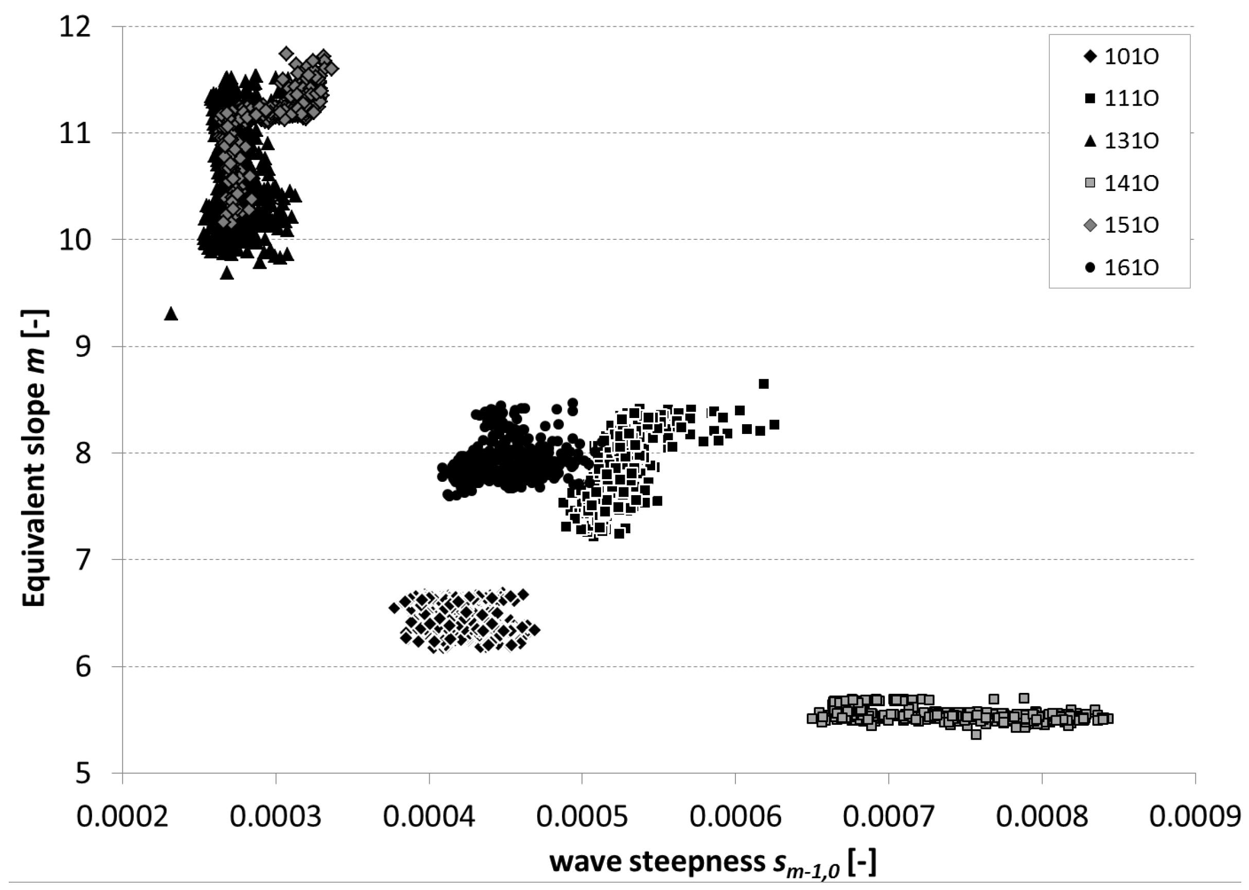
Uncertainty in wave overtopping calculation using SWASH Shallow foreshore conditions (along the Flemish coast) 50 WL2017R16_011_1 Final version Figure 39 Dimensionless wave overtopping discharge Qdim results: SWASH vs. empirical equation 1 (using coefficient of eq 5: ‘MB’)

Uncertainty in wave overtopping calculation using SWASH Shallow foreshore conditions (along the Flemish coast) Final version WL2017R16_011_1 51 Figure 40 Dimensionless wave overtopping discharge Qdim results: SWASH vs. empirical equation 1 (using coefficient of eq 6: ‘Alto’)

Uncertainty in wave overtopping calculation using SWASH Shallow foreshore conditions (along the Flemish coast) 52 WL2017R16_011_1 Final version Figure 41 - Ratio of wave overtopping discharge Qdim between SWASH and equation eqdet 5 in relation to the dimensionless wave overtopping discharge modelled by SWASH

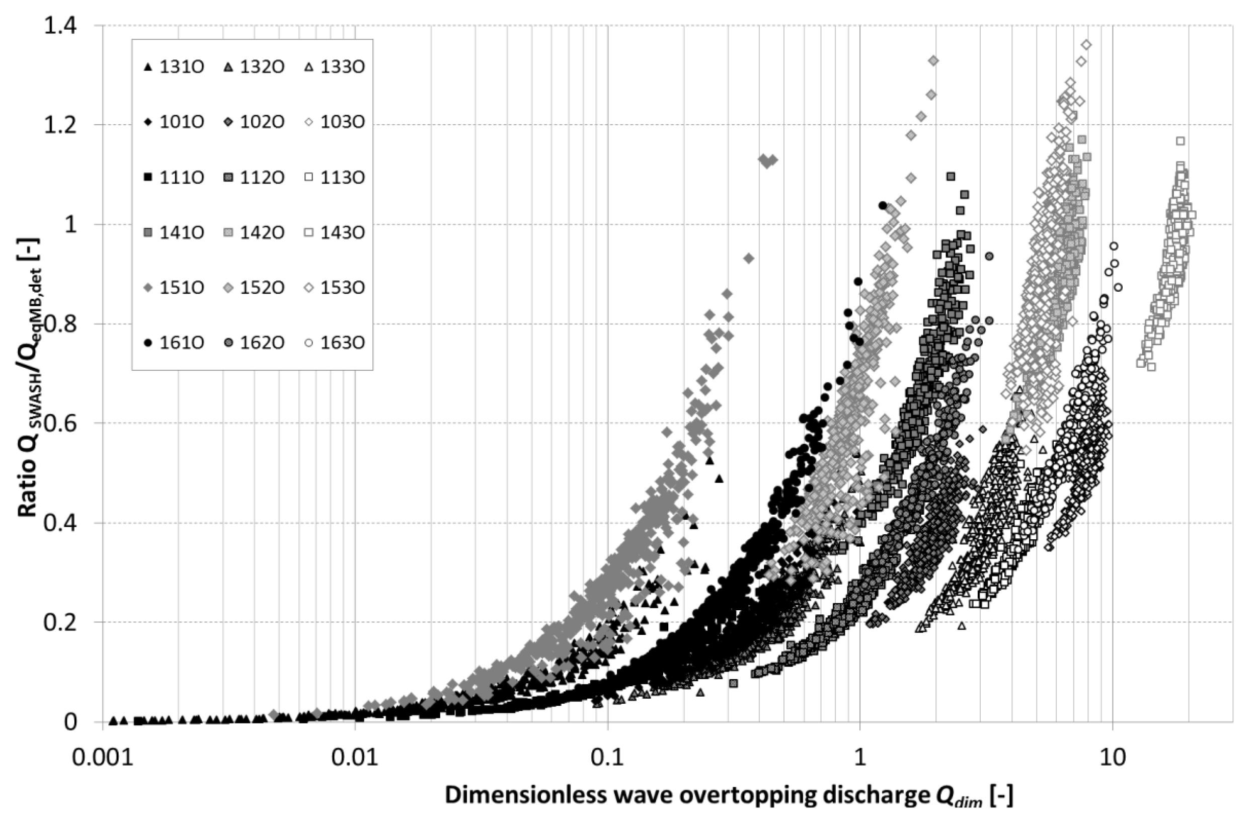
Uncertainty reduction in wave overtopping

Uncertainty in wave overtopping calculation using SWASH Shallow foreshore conditions (along the Flemish coast)

Given the crest of the dike at 9 m TAW, cases 131 and 151, having a uniform mild foreshore slope of 1/50, clearly result in a wider data cloud compared to the other cases, which have a steeper foreshore part closer to the dike (or a larger water depth: case 11X) and a higher dimensionless wave overtopping discharge. The latter mainly explains the difference.

Under or overestimation of the ‘perfect calibration’ result of the equation is entirely determined by the influence both wave and water level parameters have in the equation. The former being determined by the SWASH 2D mean results and fixed calibration limits, the latter depending on the calibration routine used in SWASH Consider1D.the exceptional case 15X and take 151 as an example, its selected ‘perfect calibration’ seed has an offshore calibrated water level SWL (= 7.17 m TAW) that only 6% of the other seeds also have. A deviation of 0.01 to 0.02 m on this value leads to a 2 to 4% difference on the calculated wave overtopping; being the least significant. A divergence of 0.01 to 0.02 m on the perfectly calibrated wave height Hm0 at the toe, i.e. within calibration limits, leads to a 9 to 16% difference on the calculated wave overtopping. A divergence of 1 to 2 s on the perfectly calibrated spectral wave period Tm 1,0 at the toe, being a little too high, leads to a 5 to 9% difference on the calculated wave overtopping. Combining these divergences (see Figure 18 and Figure 19) to the selected perfect calibration match leads to the significant overestimation visualised in Figure 42. Note that, although the magnitude of the error is case dependent, under or overestimation of the wave overtopping discharge calculated by equation is most sensitive to a deviation of the target wave parameters (Hm0, Tm 1,0) at the toe of the dike.

Final version WL2017R16_011_1 53 6

The calibration mismatch generally leads to 50% lower up to 20% higher wave overtopping results, with case 15X being the exception. Cases 10X, 14X and 16X show a rather symmetrical data cloud against the ratio equal to 1 whereas cases 11X and 13X tend to overestimate the ‘perfect’ wave overtopping result and case 15X clearly underestimates it. Under or overestimation decrease with a decreasing freeboard.

calculation using SWASH 6.1 Uncertainty source 1: calibration mismatch

Although the incident hydraulic boundary conditions in SWASH 1D are calibrated within rather tight limits, these calibration results do not perfectly match to the 2D results.

Figure 42 depicts the difference in wave overtopping discharge, calculated by equation 1 (including coefficients of equation 5), given a perfect and real calibrated match of the incident hydraulic boundary conditions. It is shown as the ratio qeq,perf_calib/qeq,real_calib against the SWASH dimensionless wave overtopping results. The numerator of this ratio corresponds to the wave overtopping discharge, calculated by equation 1, using the 1D incident hydraulic boundary conditions of the simulation having the perfect (closest) match to the 2D results for every parameter (see Table 7); the denominator equals the wave overtopping discharge, calculated by the same equation, using the 1D incident hydraulic boundary conditions of each Givensimulation.aspecific case, the spreading on the ratio qeq,perf_calib/qeq,real_calib becomes smaller with increasing dimensionless wave overtopping discharge and hence, smaller relative freeboard R*

54 WL2017R16_011_1 Final version

Table 7 Selected 1D

CasenumberSeed Incident hydraulic boundary conditions at the toe Calibration results Hm0 [m] Tm 1,0 [s] Wave set up [m] Hm0 [ ] Tm 1,0 [ ] Wave set up [m] 10X 261 0.78 35.02 0.09 1.00 1.02 0.00 11X 146 0.82 29.19 0.14 0.99 0.95 0.00 13X 470 0.69 39.10 0.12 1.00 1.00 0.00 14X 451 0.86 27.47 0.03 1.00 1.00 0.00 15X 79 0.68 39.37 0.13 1.00 1.03 0.00 16X 434 0.76 32.67 0.08 1.00 1.02 0.01 Table 8 Calibrated offshore hydraulic boundary conditions for 130I numberSeed Significant wave height Hm0 [m] Water level [m TAW] 47 1.93 7.17 470 2.08 7.17

Wave overtopping discharge calculated by SWASH however results from the wave transformation characteristics of a specified wave spectrum, leading to similar hydraulic boundary conditions at the toe of the dike. For example, Table 9 lists the wave overtopping results of 2 seed numbers of case 13X, both leading to a perfect calibration match (calibrated offshore hydraulic boundary conditions in Table 8). The model results differ about a factor 10, 2 and 1.5 between one another for case 131, 132 and 133 respectively. Suppose one uses the ratio to improve the calibration mismatch, both perfect calibration matches are to be multiplied by a ratio = 1, which then logically leads to the same results. Hence two wave overtopping results, differing e.g. factor 10 of one another, are both assumed to be correct. This indicates that the semi empirical equation’s structure does not grasp the uncertainty in the wave overtopping discharge like the numerical model does. Semi empirical equations are the result of data fitting on a set of physical model tests (i) that use surface elevation time series given a specified wave spectrum, which are not altered multiple times to account for the wave train’s randomness, (ii) where the model geometry generally represents a simplified real bathymetry and (iii) that exhibit model and scale effects

Uncertainty in wave overtopping calculation using SWASH Shallow foreshore conditions (along the Flemish coast)

To conclude, both methods (SWASH and semi empirical equation) include uncertainties and inaccuracies; hence, it is not wise to ‘improve’ one approach using the other without knowing which one corresponds the best to reality. simulations having a perfect calibration match of incident hydraulic boundary conditions to the 2D results

Uncertainty in wave overtopping calculation using SWASH Shallow foreshore conditions (along the Flemish coast) Final version WL2017R16_011_1 55 Table 9 - Difference in the SWASH and equation wave overtopping results given 2 perfect calibration matches Seed number Case 131 Case 132 Case 133 Modelled wave dischargeovertoppingqSWASH [l/s/m] 47 0.03 0.60 4.91 470 0.23 1.43 7.22 Calculated wave dischargeovertoppingqeq, prob 5 [l/s/m] 47 0.56 2.07 7.62 470 0.55 2.02 7.44 Figure 42 - Ratio of wave overtopping discharge q, calculated by equation, given a perfect and real calibrated match of incident hydraulic boundary conditions in relation to the dimensionless wave overtopping discharge Qdim modelled by SWASH

If we consider the safety assessment’s wave overtopping limit, i.e. q = 1 l/s/m, a SWASH wave overtopping result of 0.7 l/s/m leads to 0.99 ≈ 1.0 l/s/m.

��

Translating this relation to a confidence band around the mean, Figure 44 illustrates that 68.3% of the wave overtopping values are captured within ± 1σ around the mean and 90% of them within ± 1.64σ. The former’s upper confidence band, i.e. µ + σ, is generally used as the ‘deterministic’, safer result for design and assessment purposes.

��+1��

Uncertainty in wave overtopping calculation using SWASH Shallow foreshore conditions (along the Flemish coast) 56 WL2017R16_011_1 Final version 6.3 Uncertainty source 2: seed number

As stated in Section 2.3, starting from one wave spectrum, every seed number develops a specific wave train, which differs in sequence of the individual waves from another, leading to different volumes of waves that overtop and hence, a possible different wave overtopping discharge.

Given that wave overtopping is accepted to be normally distributed (cf. Section 4.3.4), its mean and variability, or uncertainty, around this value can be assessed by its relative error (equation 12). The higher the mean wave overtopping, the lower the relative error becomes (power law relation, Figure 43).

To account for the seed variability, a wave overtopping results needs therefore to be increased: = ∙ (1 + 1 ∙ 0 3655�� 0 378 ) (13) Or stated differently, the standard deviation to be added to a wave overtopping result can be calculated as: �� = 0.3655 �� 0 622 (14)

Note that the results of the one seed calibration are slightly different, i.e. ��+1�� = �� ∙ (1 + 1 ∙ 0 3227�� 0 466 ) (15) Applying both equations to the overtopping limit of 1 l/s/m, the results are however very alike, i.e. 1.37 with equation 13 and 1.32 l/s/m with equation 14 respectively (see also Figure 41 ).

Uncertainty in wave overtopping calculation using SWASH Shallow foreshore conditions (along the Flemish coast) Final version WL2017R16_011_1 57 Figure 43 - Mean wave overtopping �� in relation to its relative error σ’ (seed dependent calibration) Figure 44 - Mean wave overtopping q and its 68% and 90% confidence bands (black: seed dependent calibration; grey: one seed calibration)

Figure 45 Probabilistic and deterministic ratio of wave overtopping discharge Qdim between SWASH and equation 1 (including coefficients of eq 5: ‘eqMB’) in relation to the dimensionless wave overtopping discharge modelled by SWASH

Uncertainty in wave overtopping calculation using SWASH Shallow foreshore conditions (along the Flemish coast) 58 WL2017R16_011_1 Final version

The lower the dimensionless wave overtopping discharge Qdim, the higher logically the relative difference between probabilistic and deterministic wave overtopping discharges (cf. Figure 43) In agreement with Figure 39 and Figure 40, the ratio QSWASH/Qeq is significantly lower for case 111 (and 131) compared to case 151 while these cases lead to similar dimensionless wave overtopping discharges and have the same freeboard, i.e. 0.11 (0.05) and 0.13 respectively. The same holds for e.g. cases 101 and 161

Besides the influence of the shallow foreshore’s length on wave set up and breaking mechanisms, the re reflection and non dampening of the long waves being generated in a wave flume might cause a built up of extra wave energy (cf. Section 5.2) This leads to an even larger overestimation of wave overtopping in these physical model tests and consequently, a smaller ratio QSWASH/Qeq

Comparing the dimensionless wave overtopping discharges calculated by SWASH and semi empirical equation 1 using the coefficients of equation 5 (‘QeqMB’) and 6 (‘QeqAlto’) in a probabilistic and deterministic way (Figure 45 and Figure 46 respectively), it can be seen that the ratio between both methods decreases (i) when the dimensionless wave overtopping discharge decreases and (ii) using the deterministic method in eqs 5 and 6, compared to the probabilistic mean values. The latter indicates that the variation enclosed in the semi empirical equation’s standard deviation is larger than the one included in the SWASH seed variability’s equation.

Uncertainty in wave overtopping calculation using SWASH Shallow foreshore conditions (along the Flemish coast)

If a population is normally distributed, the two methods produce similar results; contrary, non normality is clearly visualized in the data sampling figure by the skewed sampling pattern (e.g. Figure 47C).

Data sampling randomly resamples a specified number of observations from the population; hence, without prior assumption of the underlying distribution of the population. Using a Monte Carlo approach, an identical number of observations is randomly sampled from a normal distribution, being characterized by the population’s mean and standard deviation (based on Section 4.3.4).

Figure 47 illustrates that the more observations are included in a sample, the closer the samples’ wave overtopping averages are located to one another and the smaller the samples’ spread becomes. Assuming a normal distribution, Monte Carlo samples (Figure 47B and D) are to be taken symmetrically around the distribution’s parameters and hence, negative results can be obtained (being physically impossible) Data sampling on the other hand, only samples results from the population (Figure 47A and C).

Final version WL2017R16_011_1 59

Figure 46

Probabilistic and deterministic ratio of wave overtopping discharge Qdim between SWASH and equation 1 (including coefficients of eq 6: ‘eqAlto’) in relation to the dimensionless wave overtopping discharge modelled by SWASH 6.4 Uncertainty source 3: sample size

The number of samples is set equal to 10000, the sample size varies from 1 to 20 observations.

In practice, it is often not possible to carry out such amount of simulations (here: 500) to determine the wave overtopping discharge. Applying both a Monte Carlo and data sampling approach, it is tried to quantify the added uncertainty σsample given that only a reduced sample of x wave overtopping discharges is taken out of the population

Uncertainty in wave overtopping calculation using SWASH Shallow foreshore conditions (along the Flemish coast) WL2017R16_011_1

Final version

The overall results from both sampling methods are however very similar. Figure 48 shows the mean wave overtopping discharge, i.e. the average of all samples’ means, and related error (± 1 standard deviation σ) against sample size for both the Monte Carlo and data sampling methods. For the latter method, also the results obtained with a reduced number of samples (= 100 instead of 10000) are plotted to check the robustness of the method. The mean wave overtopping discharge can be considered independent of the sample size whereas the standard deviation clearly reduces with increasing sample size. This reduction in variability however asymptotically slows down. The results for a reduced number of data samples show a little more spreading, yet follow the same trend.

Considering the mean and standard deviation of the wave overtopping discharges for this sample size in all bathymetric configurations (using the Monte Carlo and data sampling methods), a power law relation between these parameters is obtained (Figure 50) To account for the added uncertainty when using a reduced sample size of 8, its associated variability needs to be calculated as: ��sample = 0.131 ∙ �� 0 620 (16) Figure 47 Monte Carlo (B and D) and data sampling (A and C) methods: wave overtopping characteristics related to sample size A B

Figure 49, indicating this decrease of spreading around the mean value for all sample sizes, illustrates that (i) the standard deviation, being directly linked to the magnitude of the wave overtopping discharge, increases with increasing wave overtopping discharge (e.g. OVT101 = 0.8 l/s/m OVT 103: 17 l/s/m) and (ii) as from a sample size of 8 to 10 the added accuracy to be gained becomes insignificant compared to the calculation effort of doing extra simulations. Therefore, a sample size of 8 is opted for. Appendix 3 lists the results of the other cases.

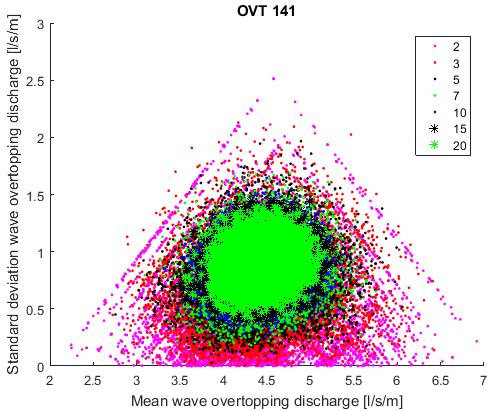
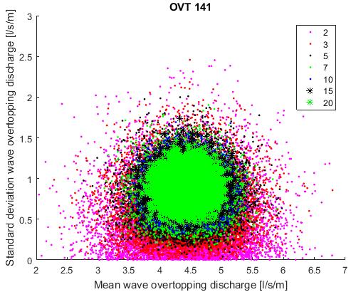
Uncertainty in wave overtopping calculation using SWASH Shallow foreshore conditions (along the Flemish coast) Final version WL2017R16_011_1 61 Figure 48 Wave overtopping characteristics: mean and standard deviation against sample size for Monte Carlo (MC) and data sampling methods (DS red: reduced number of samples = 100) C D

Uncertainty in wave overtopping calculation using SWASH Shallow foreshore conditions (along the Flemish coast) 62 WL2017R16_011_1 Final version Figure 49 Standard deviation on wave overtopping discharge against sample size for Monte Carlo (MC) and data sampling methods (DS red: reduced number of samples = 100): cases 10X and 15X

Figure 50 Relation between mean and standard deviation of wave overtopping discharge sample size: 8 Besides, the identical results of the two sampling methods point out that the non normality of some of the wave overtopping populations can be nicely approximated by the population’s normal distribution on the condition that the number of observations is large enough (cf. central limit theorem in Section 4.3.4).

then: �� = ∑�� =1 �� (17) In

Ideally, 500 simulations should be carried out when a low wave overtopping discharge is to be expected. 8 simulations already reduce the uncertainty to an acceptable level Figure Figure

need

Therefore, these

32 and

the standard deviation to be

quadrature: �� = ��seed 2 + ��sample 2 � (18) In which: σseed

The uncertainties enclosed in either the seed number selection or the sampling size choice are independent of one another. This implies that their introduced error is just as likely to (partially) cancel out the other one, as it is to add uncertainty to it. errors to be combined in is the standard deviation be derived is derived result: wave overtopping

The final wave overtopping discharge is calculated

Uncertainty in wave overtopping calculation using SWASH Shallow foreshore conditions (along the Flemish coast) Final version WL2017R16_011_1 63 6.5 Using SWASH for wave overtopping calculation: accounting for uncertainty sources Different sources of uncertainty need to be accounted for in the SWASH wave overtopping results, in a stepwise approach 1. Number of simulations to calculate wave overtopping

Practically,

from equation 14; σsample

33).

as: ��,�� = �� + �� (19)

2. Accounting for seed and sample size uncertainty

(cf.

The mean wave overtopping discharge �� is which: is the number of simulations.

from equation 16. 3. End

It was investigated whether or not a SWASH wave overtopping result can be optimized by multiplying it with the ratio qeq,perf/qeq,calib in order to account for this calibration mismatch. The numerator of this ratio corresponds to the wave overtopping discharge, calculated by the relevant semi empirical equation (to be found in Allsop et al., 2016), using the 1D incident hydraulic boundary conditions of the simulation having the perfect (closest) match to the 2D results for every parameter; the denominator equals the wave overtopping discharge, calculated by the same equation, using the 1D incident hydraulic boundary conditions of the simulation to be optimized. Given a specific case, the spreading on the ratio qeq,perf/qeq,calib became smaller with increasing dimensionless wave overtopping discharge and hence, smaller relative freeboard R*

The methodology comprised three successive steps to be followed. First, wave transformation was modelled 300 times for every bathymetric configuration in order to obtain an average of incident hydraulic boundary conditions at the toe of the dike (significant wave height Hm0, spectral wave period Tm 1,0, still water level SWL and wave set up), which are considered to be the reference values for that configuration

This study aimed at quantifying sources of uncertainty in wave overtopping calculation using SWASH 1D, which then could be translated into a safety factor, to be added to the SWASH results. The focus was on shallow foreshore conditions, prevalent along the Flemish coast, which are characterized by specific wave transformation processes such as heavy wave breaking and ‘surf beat’ infragravity wave motion. Six bathymetric configurations were considered, varying in cross shore profile, in foreshore length, in presence of a steeper part in its slope closer to the dike,…

1. Calibration mismatch

Although the incident hydraulic boundary conditions in SWASH 1D are calibrated within rather tight limits, these calibration results do not perfectly match to the 2D reference values

Uncertainty in wave overtopping calculation using SWASH Shallow foreshore conditions (along the Flemish coast) 64 WL2017R16_011_1 Final version 7 Conclusion & outlook 7.1 Conclusion

A deviation of the target wave parameters (Hm0, Tm 1,0) at the toe of the dike led to the highest under or overestimation of the ‘perfect calibration’ wave overtopping calculated by equation Applying an equation however, identical incident hydraulic boundary conditions at the toe lead to an identical wave overtopping discharge. Contrary, two perfectly calibrated simulations in SWASH 1D lead possibly to different wave overtopping discharges Both methods include uncertainties and inaccuracies; hence, it is not wise to ‘improve’ one approach using the other without knowing which one corresponds the best to reality.

2. Difference in surface elevation time series: seed number

Second, the incident hydraulic boundary conditions at that toe were calibrated for 500 SWASH 1D simulations (per bathymetric configuration) against these reference values. Third, wave overtopping discharge was estimated by these 500 ‘calibrated’ SWASH 1D simulations for the 3 cases, i.e. different crest levels, of a dike configuration

Making use of these wave overtopping results, the mean wave overtopping discharge was calculated and three sources of uncertainty were identified:

Selecting a seed number assigns randomly a starting phase, being part of a population of uniformly distributed random phases, to all harmonic components. The resulting wave train, which differs in individual wave sequence from another, leads to different volumes of waves that overtop and hence, a possible different wave overtopping discharge.

�� = ∑ ��,�� 8 �� =1 ��

To account for the seed variability, a wave overtopping result needs to be increased by: Sample size

version WL2017R16_011_1 65

Given that wave overtopping discharge is accepted to be normally distributed, its mean and variability around this value can be assessed by its relative error The higher the mean wave overtopping discharge , the lower the relative error becomes (power law relation). Translating this relation to a confidence band around the mean indicates that 68.3% of the wave overtopping values are captured within ± 1 standard deviation around the mean. The upper confidence limit, i.e. �� + σ, is generally used for design and assessment purposes, adding some safety to the mean result.

131 ∙ ��

To conclude, wave overtopping discharge needs to be estimated by at least 8 SWASH 1D simulations. Their average result: is then the wave overtopping discharge on which for seed and sample size uncertainty needs to be accounted. Given that the uncertainties enclosed in either the seed number selection or the sample size choice are independent of one another, these errors are to be combined in quadrature: This leads to a final wave overtopping discharge: Outlook further research

This study demonstrated that: Not only the incident wave parameters at the toe of the dike, i.e. the significant wave height Hm0 and spectral wave period Tm 1,0, are important for wave overtopping but also the still water level including wave set up. Especially in (very) shallow foreshore conditions, a long surf zone can be present where wave set up and breaking mechanisms influence the local conditions (cf. SWASH 2D results)Translating a synthetic sea state into an infinite (here: 500) number of surface elevation time series indicated that the maximum wave height, wave sequence and groupiness factor affect wave overtopping significantly (when the relative freeboard is higher than 1.6)

��,�� = �� + �� 7.2

Uncertainty in wave overtopping calculation using SWASH Shallow foreshore conditions (along the Flemish coast)

��

��+1�� = �� (1 + 1 0.3655�� 0 378 ) 3.

To account for the added uncertainty of this reduced sample size, its associated variability needs to be calculated as: sample = 0 0 620

�� = ��seed 2 + ��sample 2 �

As from a sample size of 8 to 10 the added accuracy to be gained by increasing the sample size became insignificant compared to the calculation effort of doing extra simulations. Therefore, a sample size of 8 was opted for.

��

Final

σ’.

In practice, it is often not possible to carry out that amount of simulations to determine the wave overtopping discharge . Applying both a Monte Carlo and data sampling approach, the added uncertainty sample was quantified given that only a reduced sample of 1 to 20 q’s is taken out of the population

Uncertainty in wave overtopping calculation using SWASH Shallow foreshore conditions (along the Flemish coast)

With regard to the calibration, it is important to note that: Given a certain seed, various offshore parameter combinations might lead to a calibration match with the 2D reference values. A different parameter combination possibly leads to another wave overtopping discharge (depending on the relative freeboard)

Wave overtopping is calculated using a test duration of about 500 peak wave period. For higher relative freeboards, i.e. above 1.6, a longer test duration is preferred to avoid the result is adversely influenced

Given that SWASH 2D is still unstable for a combined wave transformation and overtopping calculation (Suzuki et al., 2017), a procedure is proposed to calibrate the SWASH 1D hydraulic conditions at the toe of the dike to the 2D values at that location. Focus is hereby put on obtaining a similar wave spectrum (and hence, wave parameters) and water level as in the 2D situation (in line with the parameters applied in a semi empirical wave overtopping equation).

66 WL2017R16_011_1 Final version

Offshore significant wave height is roughly half and the water level is slightly higher compared to the 2D values. This implies that the surf zone is significantly shorter and hence, wave set up and breaking mechanisms different Further validation (or improvement) of this procedure is recommended.

8 References

Uncertainty in wave overtopping calculation using SWASH Shallow foreshore conditions (along the Flemish coast) WL2017R16_011_1 67 Allsop, N.W..; Bruce, T.; De Rouck, J.; Kortenhaus, A.; PUllen, T.; Schüttrumpf, H.; Troch, P.; van der Meer, J.W.; Zannutigh, B. (2016). EurOtop. Manual on wave overtopping of sea defences and related structures. 2nd edition Altomare, C.; Suzuki, T.; Chen, X.; Verwaest, T.; Kortenhaus, A. (2016). Wave overtopping of sea dikes with very shallow foreshores. Coast. Eng. An Int. J. Coastal, Harb. Offshore Eng. 116. Available at: http://hdl.handle.net/10.1016/j.coastaleng.2016.07.002

Kamphuis, J.W. (1998). Long waves in flume experiments, in: (1998). pp. 1154 1167

Altomare, C.; Suzuki, T.; Dan, S.; Peeters, P.; Mostaert, F. (2017). Raversijde Mariakerke Wellington west Wave overtopping and wave forces. Results from experimental campaigns.Version 5. FHR Reports, 13_168_1. Flanders Hydraulics Research: Antwerpen. Version 5. Battjes, J.A.; Groenendijk, H.W. (2000). Wave height distribution on shallow foreshores p 161 182. doi:10.1016/S0378 3839(00)00007 7 De Bakker, A.T.M.; Tissier, M.F.S.; Ruessink, B.G. (2014). Shoreline dissipation of infragravity waves. Cont. Shelf Res. 72: 73 82. doi:10.1016/j.csr.2013.11.013

Kortenhaus, A.; Oumeraci, H.; Geeraerts, J.; Rouck, J.D.E.; Medina, J.R. (2004). Laboratory effects and further uncertainties associated with wave overtopping measurements., in: (2004). pp. 4456 4468 McCabe, M. V.; Stansby, P.K.; Apsley, D.D. (2013). Random wave runup and overtopping a steep sea wall: Shallow water and Boussinesq modelling with generalised breaking and wall impact algorithms validated against laboratory and field measurements. Coast. Eng. ISBN 0378 3839 74: 33 49. doi:10.1016/j.coastaleng.2012.11.010 Meurisse, F.; Mesu, K.V. (2017). Experimental study of overtopping performance of steep low crested structures with rough elements. Ghent University Pullen, T.; Allsop, N.; Bruce, T.; Kortenhaus, A.; Schüttrumpf, H.; Van der Meer, J.W. (2007). EurOtop. Wave Overtopping of Sea Defences and Related Structures: assesment manual. ISBN 9783804210646 1 171 Rijnsdorp, D.P.; Smit, P.B.; Zijlema, M. (2014). Non hydrostatic modelling of infragravity waves under

Final version

De Roo, S.; Suzuki, T.; Vanneste, D.; Peeters, P.; Mostaert, F. (2017). Safety assessment 2015 testcase. Execution of the test case and evaluation of the contractor’s.Version 2.. WL Rapporten, 14_014_X. Flanders Hydraulics Research: Antwerpen. Version 2. De Roo, S.; Trouw, K.; Ruiz Parrado, I.; Suzuki, T.; Verwaest, T.; Mostaert, F. (2016). Het Hydraulisch randvoorwaardenboek (2014). WL Rapporten, 14_014. Waterbouwkundig Laboratorium/Fides Engineering: Antwerpen Goda, Y. (2009). Derivation of unified wave overtopping formulas for seawalls with smooth , impermeable surfaces based on selected CLASH datasets. Coast. Eng. 56(4): 385 399. doi:10.1016/j.coastaleng.2008.09.007 Guza, R.T.; Feddersen, F. (2012). Effect of wave frequency and directional spread on shoreline runup. Geophys. Res. Lett. ISBN 0094 8276 39(11): 1 5. doi:10.1029/2012GL051959 Herbers, T.H.C.; Elgar, S.; Guza, R.T. (1999). Directional spreading of waves in the nearshore zone. J. Geophys. Res. ISBN 0029 8018 104: 7683 7693. doi:10.1029/1998JC900092

Smit, P.; Zijlema, M.; Stelling, G. (2013). Depth induced wave breaking in a non hydrostatic, near shore wave model. Coast. Eng. 76: 1 16. doi:10.1016/j.coastaleng.2013.01.008

Uncertainty in wave overtopping calculation using SWASH Shallow foreshore conditions (along the Flemish coast) 68 WL2017R16_011_1 Final version laboratory conditions. Coast. Eng. 85: 30 42. doi:10.1016/j.coastaleng.2013.11.011

Methodology for safety assessment 2015 Background report on wave transformation and overtopping calculation by SWASH. FHR Reports, 14_014_6. Flanders Hydraulics Research: Antwerp Suzuki, T.; Altomare, C.; Veale, W.; Verwaest, T.; Trouw, K.; Troch, P.; Zijlema, M. (2016). Efficient and robust wave overtopping estimation for impermeable coastal structures using SWASH. Coast. Eng. (122): 108 123. doi:10.1016/j.coastaleng.2017.01.009

Suzuki, T.; Altomare, C.; De Roo, S.; Kolokythas, G.K.; Vanneste, D.; Peeters, P.; Mostaert, F. (2017).

Romano, A.; Bellotti, G.; Briganti, R.; Franco, L. (2015). Uncertainties in the physical modelling of the wave overtopping over a rubble mound breakwater: The role of the seeding number and of the test duration. Coast. Eng. 103: 15 21. doi:10.1016/j.coastaleng.2015.05.005

Ruiz Parrado, I.; Vanneste, D.; Vanderkimpen P.; Verwaest, T.; Peeters, P.; Mostaert, F. (2017). Update Flood Risk Coastal Plain 2015. Flood modeling report. WL Rapporten, 14_150_1. Flanders Hydraulics Research Smit, P.; Janssen, T.; Holthuijsen, L.; Smith, J. (2014). Non hydrostatic modeling of surf zone wave dynamics. Coast. Eng. ISBN 0378 3839 83: 36 48. doi:10.1016/j.coastaleng.2013.09.005

Suzuki, T.; De Roo, S.; Altomare, C.; Zhao, G.; Kolokythas, G.K.; Willems, M.; Verwaest, T.; Mostaert, F. (2016). Toetsing kustveiligheid 2015 Methodologie: toetsingsmethodologie voor dijken en duinenVersie 10. WL Rapporten, 14_014. Waterbouwkundig Laboratorium: Antwerpen. Versie 10. van Dongeren, A.; Battjes, J.; Janssen, T.; van Noorloos, J.; Steenhauer, K.; Steenbergen, G.; Reniers, A. (2007). Shoaling and shoreline dissipation of low frequency waves. J. Geophys. Res. Ocean. ISBN 9789812562982 112(2): 1 15. doi:10.1029/2006JC003701 van Gent, M.R.A. (1999). Physical model investigations on coastal structures with shallow foreshores van Vledder, G.; Ruessink, G.; Rijnsdorp, D. (2013). Individual wave height distributions in the coastal zone: Measurements and simulations and the effect of directional spreading. Coast. Dyn. 1799 1810. doi:10.1128/JCM.00586 13 Vanpoucke, P.; Reyns, J.; Van der Biest, K.; Verwaest, T.; Mostaert, F. (2009). Overstromingsrisico’s aan de Vlaamse kust: overstromingsrisico’s in de aandachtszones. WL Rapporten, 718_02j. Waterbouwkundig Laboratorium: Antwerpen Williams, H.E.; Briganti, R.; Pullen, T. (2014). The role of offshore boundary conditions in the uncertainty of numerical prediction of wave overtopping using non linear shallow water equations. Coast. Eng. 89: 30 44. doi:10.1016/j.coastaleng.2014.03.003 Zijlema, M.; Stelling, G.; Smit, P. (2011). SWASH: An operational public domain code for simulating wave fields and rapidly varied flows in coastal waters. Coast. Eng. ISBN 0378 3839 58(10): 992 1012. doi:10.1016/j.coastaleng.2011.05.015

Uncertainty in wave overtopping calculation using SWASH Shallow foreshore conditions (along the Flemish coast) Final version WL2017R16_011_1 A1 Appendix 1: Sources of post storm bathymetries Table 10 Sources of post storm bathymetries Coastal area Coastalsection Model Source De Panne 15, 18 Durosta Ruiz Parrado et al., 2016 Sint Idesbald 21 25 Durosta Until CS 22: Ruiz Parrado et al., 2016 As from CS 23: Vanpoucke et al., 2009 Koksijde 26 34 Durosta Vanpoucke et al., 2009 Westende De Krokodille Middelkerke 73 88 XBeach De Roo et al., 2017 Raversijde Mariakerke 99 108 XBeach Altomare et al., 2017 Oostende 109 116 Durosta Ruiz Parrado et al., 2016 Blankenberge 185 194 Durosta Vanpoucke et al., 2009 Knokke 233 244 Durosta Vanpoucke et al., 2009

Note that, although in some of the Figures ‘LOG_OVT1XX’ is indicated in the axis, the natural logarithm of the data was taken and statistically analysed.

In this Appendix, descriptive statistics of the wave overtopping data (seed dependent calibration) is presented: Histogram

Uncertainty in wave overtopping calculation using SWASH Shallow foreshore conditions (along the Flemish coast) A2 WL2017R16_011_1 Final version Appendix 2: Wave

Normal Q Q plot

The purpose of these descriptive statistics is to evaluate whether or not the data follow a (log)normal distribution, being the common distribution for wave overtopping data.

OVT101 .056 423 .003 .977 423 .000 a. Lilliefors Significance Correction

Test of Normality: Kolmogorov Smirnov

The0.05.Kolomogorov

Smirnov test evaluates whether the empirical distribution function of the population is close enough to the cumulative distribution function of the reference distribution.

The Shapiro Wilk test evaluates whether the points in the normal Q Q plot lie on a straight line.

Table 11 Tests of normality for wave overtopping data of case 101 Tests of Normality Kolmogorov Smirnova Wilk Statistic df Sig. Statistic df Sig.

Shapiro

A histogram represents the distribution of the data, indicating the frequencies of observations corresponding to a certain range of data values.

The quantile quantile plot is a graphical technique to assess if a data set plausibly follows a specific theoretical distribution, here: a normal distribution. The expected quantiles underlying a normal distribution are plotted against the observed quantiles. If both sets of quantiles come from the same distribution, the points lie (roughly) on a straight line.

Test of Normality: Shapiro Wilk

When testing for normality, the null hypothesis is that the population is normally distributed. The significance of the test (‘Sig.’ in the table), i.e. the p value, is then higher than the chosen alpha level, here:

descriptiveovertopping:statistics

Uncertainty in wave overtopping calculation using SWASH Shallow foreshore conditions (along the Flemish coast) Final version WL2017R16_011_1 A3 Figure 51 Histogram of the wave overtopping data of case 101 Figure 52 Normal Q Q plot of wave overtopping data of case 101

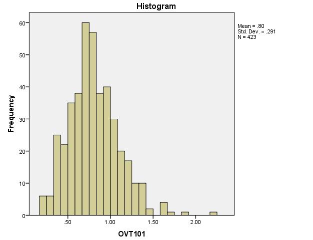
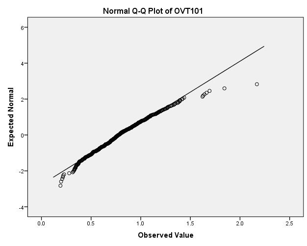
Uncertainty in wave overtopping calculation using SWASH Shallow foreshore conditions (along the Flemish coast) A4 WL2017R16_011_1 Final version Table 12 Tests of normality for ln(wave overtopping) data of case 101 Tests of Normality Kolmogorov Smirnova Shapiro Wilk Statistic df Sig. Statistic df Sig. LOG_OVT101 .073 423 .000 .975 423 .000 a. Lilliefors Significance Correction Figure 53 Histogram of the ln(wave overtopping) data of case 101

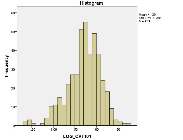
Uncertainty in wave overtopping calculation using SWASH Shallow foreshore conditions (along the Flemish coast) Final version WL2017R16_011_1 A5 Figure 54 Rankits Q Q plot of the ln(wave overtopping) data of case 101 Table 13 Tests of normality for wave overtopping data of case 102 Tests of Normality Kolmogorov Smirnova Shapiro Wilk Statistic df Sig. Statistic df Sig. OVT102 .036 450 .191 .995 450 .165 a. Lilliefors Significance Correction

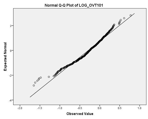
Uncertainty in wave overtopping calculation using SWASH Shallow foreshore conditions (along the Flemish coast) A6 WL2017R16_011_1 Final version Figure 55 Histogram of the wave overtopping data of case 102 Figure 56 Normal Q Q plot of the wave overtopping data of case 102

Uncertainty in wave overtopping calculation using SWASH Shallow foreshore conditions (along the Flemish coast) Final version WL2017R16_011_1 A7 Table 14 Tests of normality for wave overtopping data of case 103 Tests of Normality Kolmogorov Smirnova Shapiro Wilk Statistic df Sig. Statistic df Sig. OVT103 .039 457 .094 .987 457 .000 a. Lilliefors Significance Correction Figure 57 Histogram of the wave overtopping data of case 103

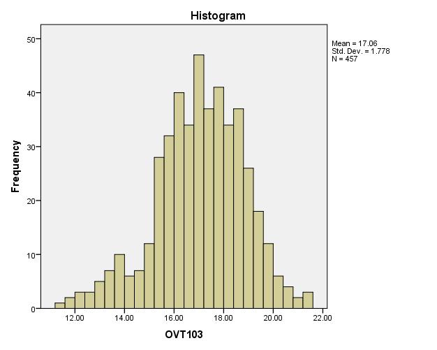
Uncertainty in wave overtopping calculation using SWASH Shallow foreshore conditions (along the Flemish coast) A8 WL2017R16_011_1 Final version Figure 58 Normal Q Q plot of the wave overtopping data of case 103 Table 15 Tests of normality for wave overtopping data of case 111 Tests of Normality Kolmogorov Smirnova Shapiro Wilk Statistic df Sig. Statistic df Sig. OVT111 .081 414 .000 .930 414 .000 a. Lilliefors Significance Correction

Uncertainty in wave overtopping calculation using SWASH Shallow foreshore conditions (along the Flemish coast) Final version WL2017R16_011_1 A9 Figure 59 Histogram of the wave overtopping data of case 111 Figure 60 Normal Q Q plot of the wave overtopping data of case 111

Uncertainty in wave overtopping calculation using SWASH Shallow foreshore conditions (along the Flemish coast) A10 WL2017R16_011_1 Final version Table 16 Tests of normality for ln(wave overtopping) data of case 111 Tests of Normality Kolmogorov Smirnova Shapiro Wilk Statistic df Sig. Statistic df Sig. LN_OVT111 .066 414 .000 .931 414 .000 a. Lilliefors Significance Correction Figure 61 Histogram of the ln(wave overtopping) data of case 111

Uncertainty in wave overtopping calculation using SWASH Shallow foreshore conditions (along the Flemish coast) Final version WL2017R16_011_1 A11 Figure 62 Normal Q Q plot of the ln(wave overtopping) data of case 111 Table 17 Tests of normality for wave overtopping data of case 112 Tests of Normality Kolmogorov Smirnova Shapiro Wilk Statistic df Sig. Statistic df Sig. OVT112 .045 397 .051 .990 397 .008 a. Lilliefors Significance Correction

Uncertainty in wave overtopping calculation using SWASH Shallow foreshore conditions (along the Flemish coast) A12 WL2017R16_011_1 Final version Figure 63 Histogram of the wave overtopping data of case 112 Figure 64 Normal Q Q plot of the wave overtopping data of case 112

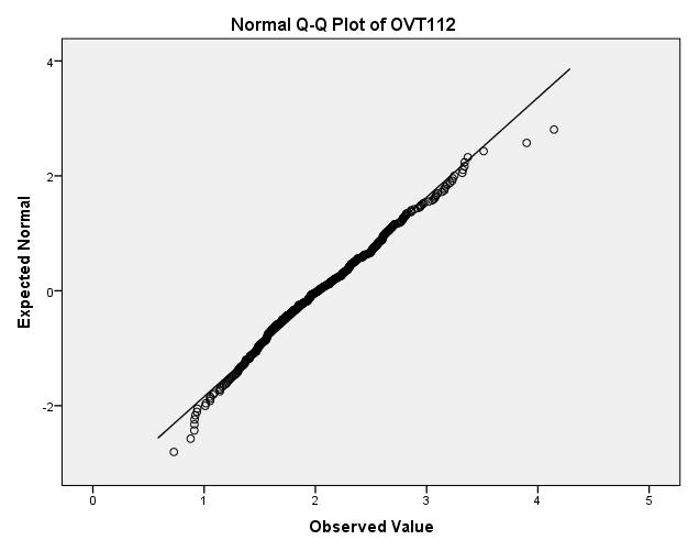
Uncertainty in wave overtopping calculation using SWASH Shallow foreshore conditions (along the Flemish coast) Final version WL2017R16_011_1 A13 Table 18 Tests of normality for ln(wave overtopping) data of case 112 Tests of Normality Kolmogorov Smirnova Shapiro Wilk Statistic df Sig. Statistic df Sig. LOG_OVT112 .058 397 .002 .985 397 .000 a. Lilliefors Significance Correction Figure 65 Histogram of the ln(wave overtopping) data of case 112

Uncertainty in wave overtopping calculation using SWASH Shallow foreshore conditions (along the Flemish coast) A14 WL2017R16_011_1 Final version Figure 66 Normal Q Q plot of the ln(wave overtopping) data of case 112 Table 19 Tests of normality for wave overtopping data of case 113 Tests of Normality Kolmogorov Smirnova Shapiro Wilk Statistic df Sig. Statistic df Sig. OVT113 .057 423 .002 .987 423 .001 a. Lilliefors Significance Correction

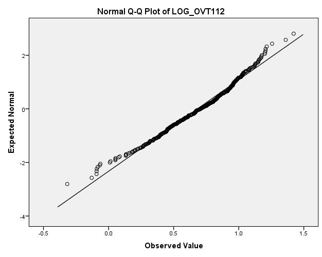
Uncertainty in wave overtopping calculation using SWASH Shallow foreshore conditions (along the Flemish coast) Final version WL2017R16_011_1 A15 Figure 67 Histogram of the wave overtopping data of case 113 Figure 68 Normal Q Q plot of the wave overtopping data of case 113

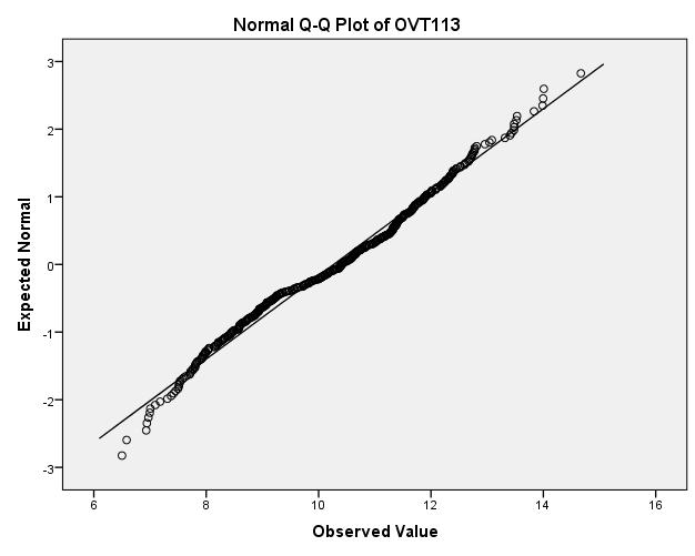
Uncertainty in wave overtopping calculation using SWASH Shallow foreshore conditions (along the Flemish coast) A16 WL2017R16_011_1 Final version Table 20 Tests of normality for ln(wave overtopping) data of case 113 Tests of Normality Kolmogorov Smirnova Shapiro Wilk Statistic df Sig. Statistic df Sig. LOG_OVT113 .078 423 .000 .978 423 .000 a. Lilliefors Significance Correction Figure 69 Histogram of the ln(wave overtopping) data of case 113

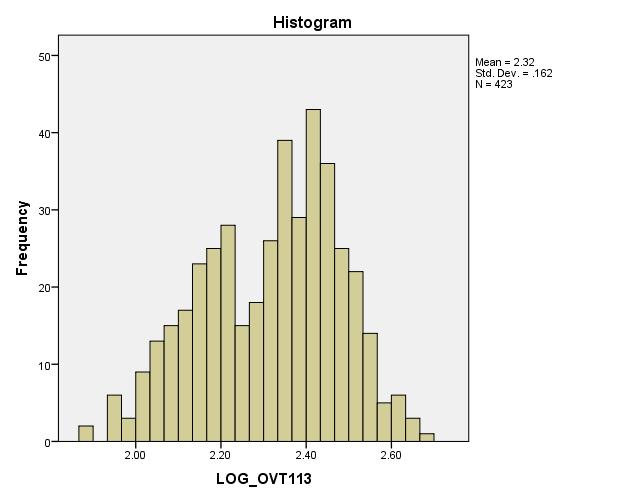
Uncertainty in wave overtopping calculation using SWASH Shallow foreshore conditions (along the Flemish coast) Final version WL2017R16_011_1 A17 Figure 70 Normal Q Q plot of the ln(wave overtopping) data of case 113 Table 21 Tests of normality for wave overtopping data of case 131 Tests of Normality Kolmogorov Smirnova Shapiro Wilk Statistic df Sig. Statistic df Sig. OVT131 .160 449 .000 .825 449 .000 a. Lilliefors Significance Correction

Uncertainty in wave overtopping calculation using SWASH Shallow foreshore conditions (along the Flemish coast) A18 WL2017R16_011_1 Final version Figure 71 Histogram of the wave overtopping data of case 131 Figure 72 Normal Q Q plot of the wave overtopping data of case 131

Uncertainty in wave overtopping calculation using SWASH Shallow foreshore conditions (along the Flemish coast) Final version WL2017R16_011_1 A19 Table 22 Tests of normality for ln(wave overtopping) data of case 131 Tests of Normality Kolmogorov Smirnova Shapiro Wilk Statistic df Sig. Statistic df Sig. LOG_OVT131 .167 442 .000 .676 442 .000 a. Lilliefors Significance Correction Figure 73 Histogram of the ln(wave overtopping) data of case 131

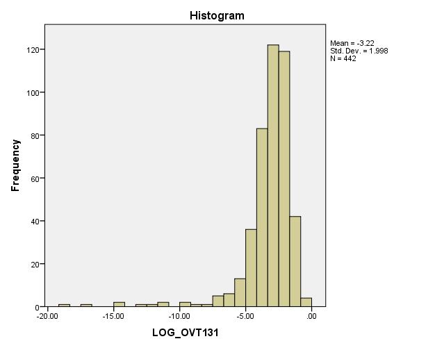
Uncertainty in wave overtopping calculation using SWASH Shallow foreshore conditions (along the Flemish coast) A20 WL2017R16_011_1 Final version Figure 74 Normal Q Q plot of the ln(wave overtopping) data of case 131 Table 23 Tests of normality for wave overtopping data of case 132 Tests of Normality Kolmogorov Smirnova Shapiro Wilk Statistic df Sig. Statistic df Sig. OVT132 .072 452 .000 .965 452 .000 a. Lilliefors Significance Correction

Uncertainty in wave overtopping calculation using SWASH Shallow foreshore conditions (along the Flemish coast) Final version WL2017R16_011_1 A21 Figure 75 Histogram of the wave overtopping data of case 132 Figure 76 Normal Q Q plot of the wave overtopping data of case 132

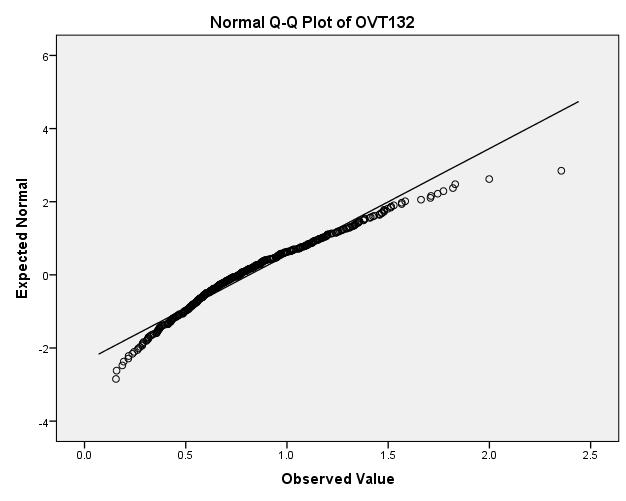
Uncertainty in wave overtopping calculation using SWASH Shallow foreshore conditions (along the Flemish coast) A22 WL2017R16_011_1 Final version Table 24 Tests of normality for ln(wave overtopping) data of case 132 Tests of Normality Kolmogorov Smirnova Shapiro Wilk Statistic df Sig. Statistic df Sig. LOG_OVT132 .033 452 .200* .986 452 .000 *. This is a lower bound of the true significance. a. Lilliefors Significance Correction Figure 77 Histogram of the ln(wave overtopping) data of case 132

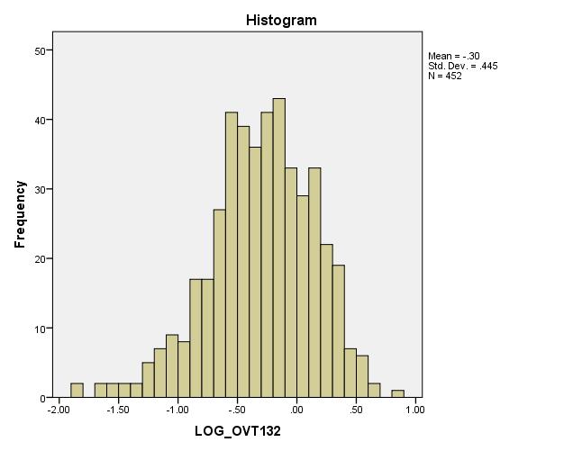
Uncertainty in wave overtopping calculation using SWASH Shallow foreshore conditions (along the Flemish coast) Final version WL2017R16_011_1 A23 Figure 78 Normal Q Q plot of the ln(wave overtopping) data of case 132 Table 25 Tests of normality for wave overtopping data of case 133 Tests of Normality Kolmogorov Smirnova Shapiro Wilk Statistic df Sig. Statistic df Sig. OVT133 .048 460 .013 .988 460 .001 a. Lilliefors Significance Correction

Uncertainty in wave overtopping calculation using SWASH Shallow foreshore conditions (along the Flemish coast) A24 WL2017R16_011_1 Final version Figure 79 Histogram of the wave overtopping data of case 133 Figure 80 Normal Q Q plot of the wave overtopping) data of case 133

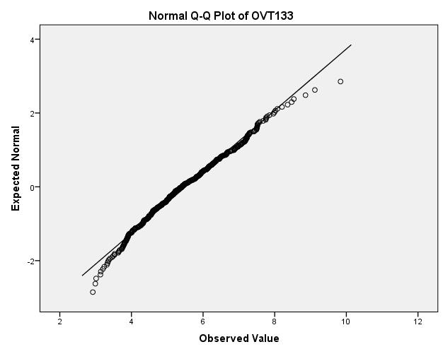
Uncertainty in wave overtopping calculation using SWASH Shallow foreshore conditions (along the Flemish coast) Final version WL2017R16_011_1 A25 Table 26 Tests of normality for ln(wave overtopping) data of case 133 Tests of Normality Kolmogorov Smirnova Shapiro Wilk Statistic df Sig. Statistic df Sig. LOG_OVT133 .039 460 .097 .993 460 .033 a. Lilliefors Significance Correction Figure 81 Histogram of the ln(wave overtopping) data of case 133

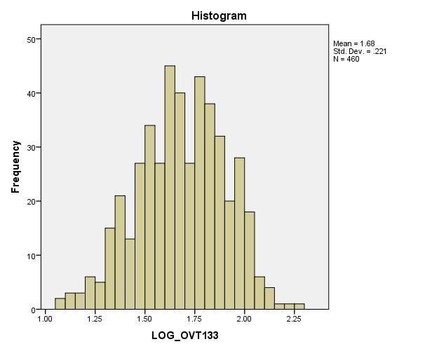
Uncertainty in wave overtopping calculation using SWASH Shallow foreshore conditions (along the Flemish coast) A26 WL2017R16_011_1 Final version Figure 82 Normal Q Q plot of the ln(wave overtopping) data of case 133 Table 27 Tests of normality for wave overtopping data of case 141 Tests of Normality Kolmogorov Smirnova Shapiro Wilk Statistic df Sig. Statistic df Sig. OVT141 .039 411 .136 .995 411 .193 a. Lilliefors Significance Correction

Uncertainty in wave overtopping calculation using SWASH Shallow foreshore conditions (along the Flemish coast) Final version WL2017R16_011_1 A27 Figure 83 Histogram of the wave overtopping data of case 141 Figure 84 Normal Q Q plot of the wave overtopping data of case 141

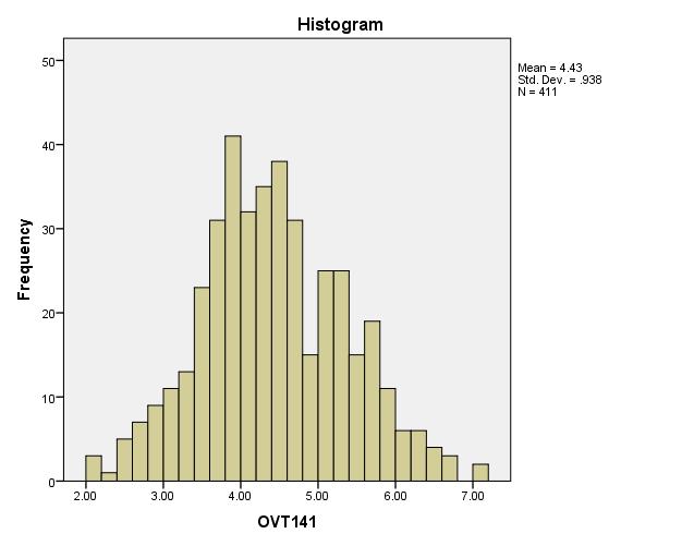
Uncertainty in wave overtopping calculation using SWASH Shallow foreshore conditions (along the Flemish coast) A28 WL2017R16_011_1 Final version Table 28 Tests of normality for wave overtopping data of case 142 Tests of Normality Kolmogorov Smirnova Shapiro Wilk Statistic df Sig. Statistic df Sig. OVT142 .035 434 .200* .994 434 .063 *. This is a lower bound of the true significance. a. Lilliefors Significance Correction Figure 85 Histogram of the wave overtopping data of case 142

Uncertainty in wave overtopping calculation using SWASH Shallow foreshore conditions (along the Flemish coast) Final version WL2017R16_011_1 A29 Figure 86 Normal Q Q plot of the wave overtopping data of case 142 Table 29 Tests of normality for wave overtopping data of case 143 Tests of Normality Kolmogorov Smirnova Shapiro Wilk Statistic df Sig. Statistic df Sig. OVT143 .043 441 .052 .985 441 .000 a. Lilliefors Significance Correction

Uncertainty in wave overtopping calculation using SWASH Shallow foreshore conditions (along the Flemish coast) A30 WL2017R16_011_1 Final version Figure 87 Histogram of the wave overtopping data of case 143 Figure 88 Normal Q Q plot of the wave overtopping data of case 143

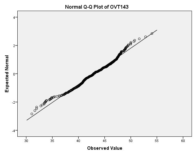
Uncertainty in wave overtopping calculation using SWASH Shallow foreshore conditions (along the Flemish coast) Final version WL2017R16_011_1 A31 Table 30 Tests of normality for ln(wave overtopping) data of case 143 Tests of Normality Kolmogorov Smirnova Shapiro Wilk Statistic df Sig. Statistic df Sig. LOG_OVT143 .051 441 .009 .969 441 .000 a. Lilliefors Significance Correction Figure 89 Histogram of the ln(wave overtopping) data of case 143

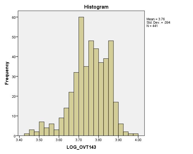
Uncertainty in wave overtopping calculation using SWASH Shallow foreshore conditions (along the Flemish coast) A32 WL2017R16_011_1 Final version Figure 90 Normal Q Q plot of the ln(wave overtopping) data of case 143 Table 31 Tests of normality for wave overtopping data of case 151 Tests of Normality Kolmogorov Smirnova Shapiro Wilk Statistic df Sig. Statistic df Sig. OVT151 .085 456 .000 .924 456 .000 a. Lilliefors Significance Correction

Uncertainty in wave overtopping calculation using SWASH Shallow foreshore conditions (along the Flemish coast) Final version WL2017R16_011_1 A33 Figure 91 Histogram of the wave overtopping data of case 151 Figure 92 Normal Q Q plot of the wave overtopping data of case 151

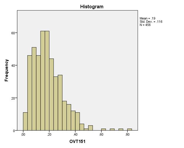
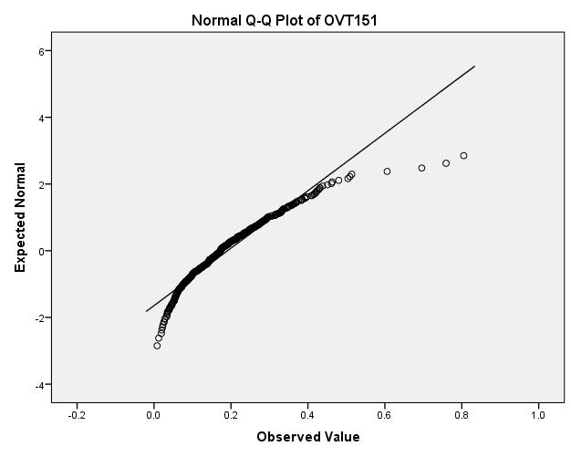
Uncertainty in wave overtopping calculation using SWASH Shallow foreshore conditions (along the Flemish coast) A34 WL2017R16_011_1 Final version Table 32 Tests of normality for ln(wave overtopping) data of case 151 Tests of Normality Kolmogorov Smirnova Shapiro Wilk Statistic df Sig. Statistic df Sig. LOG_OVT151 .083 456 .000 .967 456 .000 a. Lilliefors Significance Correction Figure 93 Histogram of the ln(wave overtopping) data of case 151

Uncertainty in wave overtopping calculation using SWASH Shallow foreshore conditions (along the Flemish coast) Final version WL2017R16_011_1 A35 Figure 94 Normal Q Q plot of the ln(wave overtopping) data of case 151 Table 33 Tests of normality for wave overtopping data of case 152 Tests of Normality Kolmogorov Smirnova Shapiro Wilk Statistic df Sig. Statistic df Sig. OVT152 .059 455 .001 .964 455 .000 a. Lilliefors Significance Correction

Uncertainty in wave overtopping calculation using SWASH Shallow foreshore conditions (along the Flemish coast) A36 WL2017R16_011_1 Final version Figure 95 Histogram of the wave overtopping data of case 152 Figure 96 Normal Q Q plot of the wave overtopping data of case 152

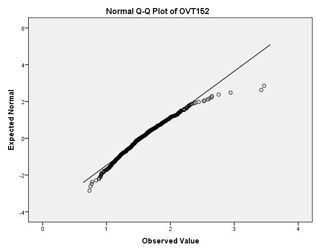
Uncertainty in wave overtopping calculation using SWASH Shallow foreshore conditions (along the Flemish coast) Final version WL2017R16_011_1 A37 Table 34 Tests of normality for ln(wave overtopping) data of case 152 Tests of Normality Kolmogorov Smirnova Shapiro Wilk Statistic df Sig. Statistic df Sig. LOG_OVT152 .027 455 .200* .997 455 .635 a. Lilliefors Significance Correction *. This is a lower bound of the true significance. Figure 97 Histogram of the ln(wave overtopping) data of case 152

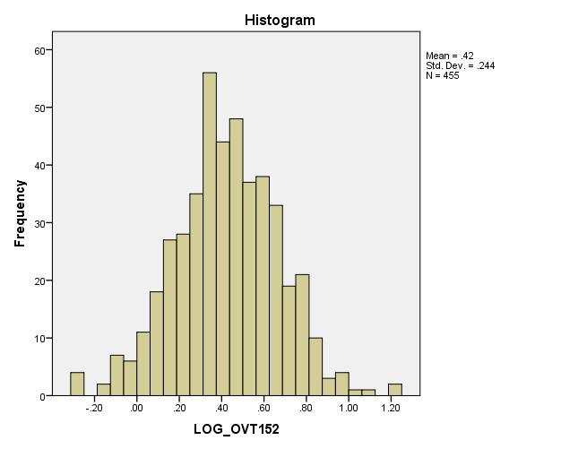
Uncertainty in wave overtopping calculation using SWASH Shallow foreshore conditions (along the Flemish coast) A38 WL2017R16_011_1 Final version Figure 98 Normal Q Q plot of the ln(wave overtopping) data of case 152 Table 35 Tests of normality for wave overtopping data of case 153 Tests of Normality Kolmogorov Smirnova Shapiro Wilk Statistic df Sig. Statistic df Sig. OVT153 .055 469 .002 .969 469 .000 a. Lilliefors Significance Correction

Uncertainty in wave overtopping calculation using SWASH Shallow foreshore conditions (along the Flemish coast) Final version WL2017R16_011_1 A39 Figure 99 Histogram of the wave overtopping data of case 153 Figure 100 Normal Q Q plot of the wave overtopping data of case 153

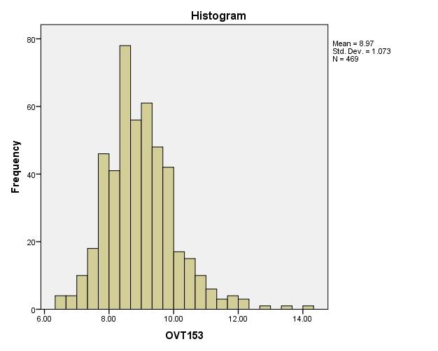
Uncertainty in wave overtopping calculation using SWASH Shallow foreshore conditions (along the Flemish coast) A40 WL2017R16_011_1 Final version Table 36 Tests of normality for ln(wave overtopping) data of case 153 Tests of Normality Kolmogorov Smirnova Shapiro Wilk Statistic df Sig. Statistic df Sig. LOG_OVT153 .036 469 .190 .991 469 .006 a. Lilliefors Significance Correction Figure 101 Histogram of the ln(wave overtopping) data of case 153

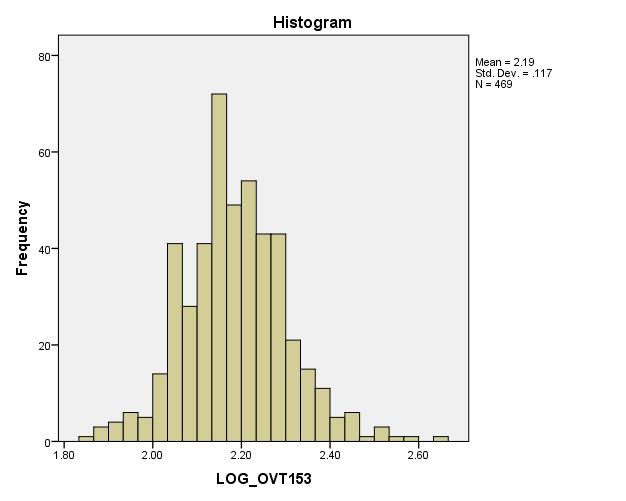
Uncertainty in wave overtopping calculation using SWASH Shallow foreshore conditions (along the Flemish coast) Final version WL2017R16_011_1 A41 Figure 102 Normal Q Q plot of the ln(wave overtopping) data of case 153 Table 37 Tests of normality for wave overtopping data of case 161 Tests of Normality Kolmogorov Smirnova Shapiro Wilk Statistic df Sig. Statistic df Sig. OVT161 .111 356 .000 .920 356 .000 a. Lilliefors Significance Correction

Uncertainty in wave overtopping calculation using SWASH Shallow foreshore conditions (along the Flemish coast) A42 WL2017R16_011_1 Final version Figure 103 Histogram of the wave overtopping data of case 161 Figure 104 Normal Q Q plot of the wave overtopping data of case 161

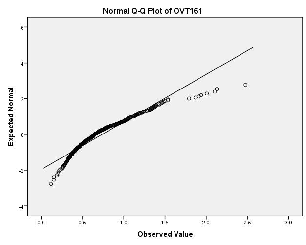
Uncertainty in wave overtopping calculation using SWASH Shallow foreshore conditions (along the Flemish coast) Final version WL2017R16_011_1 A43 Table 38 Tests of normality for ln(wave overtopping) data of case 161 Tests of Normality Kolmogorov Smirnova Shapiro Wilk Statistic df Sig. Statistic df Sig. LOG_OVT161 .035 356 .200* .995 356 .324 *. This is a lower bound of the true significance. a. Lilliefors Significance Correction Figure 105 Histogram of the ln(wave overtopping) data of case 161

Uncertainty in wave overtopping calculation using SWASH Shallow foreshore conditions (along the Flemish coast) A44 WL2017R16_011_1 Final version Figure 106 Normal Q Q plot of the ln(wave overtopping) data of case 161 Table 39 Tests of normality for wave overtopping data of case 162 Tests of Normality Kolmogorov Smirnova Shapiro Wilk Statistic df Sig. Statistic df Sig. OVT162 .088 345 .000 .959 345 .000 a. Lilliefors Significance Correction

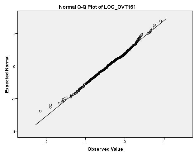
Uncertainty in wave overtopping calculation using SWASH Shallow foreshore conditions (along the Flemish coast) Final version WL2017R16_011_1 A45 Figure 107 Histogram of the wave overtopping data of case 162 Figure 108 Normal Q Q plot of the wave overtopping data of case 162

Uncertainty in wave overtopping calculation using SWASH Shallow foreshore conditions (along the Flemish coast) A46 WL2017R16_011_1 Final version Table 40 Tests of normality for ln(wave overtopping) data of case 162 Tests of Normality Kolmogorov Smirnova Shapiro Wilk Statistic df Sig. Statistic df Sig. LOG_OVT162 .038 345 .200* .992 345 .046 *. This is a lower bound of the true significance. a. Lilliefors Significance Correction Figure 109 Histogram of the ln(wave overtopping) data of case 162

Uncertainty in wave overtopping calculation using SWASH Shallow foreshore conditions (along the Flemish coast) Final version WL2017R16_011_1 A47 Figure 110 Normal Q Q plot of the ln(wave overtopping) data of case 162 Table 41 Tests of normality for wave overtopping data of case 163 Tests of Normality Kolmogorov Smirnova Shapiro Wilk Statistic df Sig. Statistic df Sig. OVT163 .082 364 .000 .952 364 .000 a. Lilliefors Significance Correction

Uncertainty in wave overtopping calculation using SWASH Shallow foreshore conditions (along the Flemish coast) A48 WL2017R16_011_1 Final version Figure 111 Histogram of the wave overtopping data of case 163 Figure 112 Normal Q Q plot of the wave overtopping data of case 163

Uncertainty in wave overtopping calculation using SWASH Shallow foreshore conditions (along the Flemish coast) Final version WL2017R16_011_1 A49 Table 42 Tests of normality for ln(wave overtopping) data of case 163 Tests of Normality Kolmogorov Smirnova Shapiro Wilk Statistic df Sig. Statistic df Sig. LOG_OVT163 .052 364 .020 .980 364 .000 a. Lilliefors Significance Correction Figure 113 Histogram of the ln(wave overtopping) data of case 163

Uncertainty in wave overtopping calculation using SWASH Shallow foreshore conditions (along the Flemish coast) A50 WL2017R16_011_1 Final version Figure 114 Normal Q Q plot of the ln(wave overtopping) data of case 163

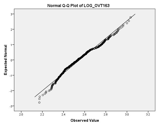
Uncertainty in wave overtopping calculation using SWASH Shallow foreshore conditions (along the Flemish coast) Final version WL2017R16_011_1 A51 Appendix 3: Wave overtopping: mean and standard deviation against sample size Table 43 Standard deviation on wave overtopping discharge against sample size for Monte Carlo (MC) and data sampling methods (DS red: reduced number of samples = 100): cases 11X, 13X, 14X and 16X

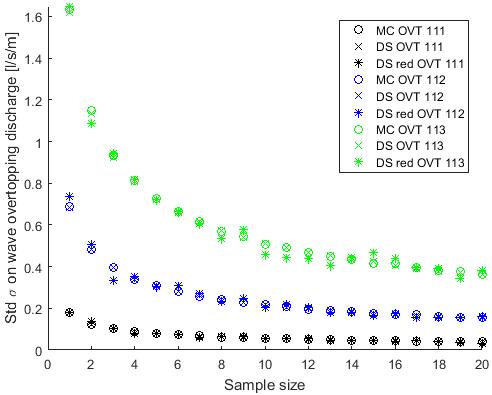
DEPARTMENT MOBILITY & PUBLIC WORKS Flanders hydraulics Research Berchemlei 115, 2140 Antwerp T +32 (0)3 224 60 35 F +32 (0)3 224 60 waterbouwkundiglabo@vlaanderen.be36 www.ﬂandershydraulicsresearch.be