
MODELLING
SKIILS Microsoft Excel, Trnsys Climate data analysis Thermal zone analysis
BUILDING ENERGY
BUILDING AND ARCHITECTURAL ENGINEERING 2015-2018 SOFTWARES
Exercise 1 – Climate Data Group 6 Andrea Battistel 854584 21/04/2016 Velmurugan Siva Kamaraj 854328
Course of Building Energy Modelling Report
Step 1 - Hourly
temperature
and
relative
humidity for the whole year
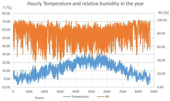
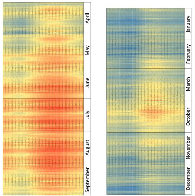
Hourly Temperature and relative humidity in the year
70.00
60.00
50.00
40.00
30.00
20.00
10.00
0.00
80.00 0 1000 2000 3000 4000 5000 6000 7000 8000 9000
80.00
60.00
40.00
100.00 -10.00
20.00
0.00
RH [%] T [°C] hours
We calculated the value of temperature and relative humidity using TRNSYS with the weather data ITMilano-Linate-160800.tm2 and plotted a graph with the hourly variation of temperature and relative humidity variation of the whole year. The hourly variation clearly shows that each day being summer or winter has it’s unique range of variation of temperature and relative humidity. Relative humidity decreases as the temperature increases which is the characterstic of moist air.
Step 2 – Comparison of Average Monthly Temperature and Radiation
We performed a simulation in TRNSYS in order to calculated the hourly values of Teperature from which is then calculated a monthly average temperature and the values obtained are compared with the standard values in UNI 10349.
Temperature RH 0.00 5.00 10.00 15.00 20.00 25.00 30.00 Temperature [ ° C] Months
Monthly Average Temperature - TRNSYS Vs UNI 10349
TRNSYS UNI
The monthly average temperature of TRNSYS is lower than the UNI 10349, it is because of the fact that the .TMY2 weather data file used for the simulation in TRNSYS is calculated as an average value for the period of 30 years ranging from 1961 to 1990 but the weather data values from UNI is calculated in the recent years.
So the monthly average temperature has increased by a value of 2 to 3 °C for each month in the span of 25 years.
As for as the Irradiations are concerned, we calculated the irradiation of the horizontal and vertical faces. The vertical face inclueds all the eight directions namely North,North-Ease,East,South-East,South,SouthWest,West,North-West.
Comparison of Irradiation on Horizontal Surface:
Horizontal Radiation TRNSYS Vs UNI
0.00 1.00 2.00 3.00 4.00 5.00 6.00 7.00
Irradiation [KWh/m 2] Months
IT_H-TRNSYS IB_H-TRNSYS ID_H-TRNSYS IT_H-UNI IB_H-UNI ID_H-UNI 0.00 1.00 2.00 3.00 4.00 5.00 6.00 7.00
Total horizontal radiation TRNSYS Vs UNI
Irradiation [KWh/m 2 ] Months
IT_H-TRNSYS IT_H-UNI
The Irradiation (Total,Beam & Diffuse) values of UNI on the horizontal surface are higher than TRNSYS due to the higher intensity of radiation exposure like we had an increase of temperature in the previous point.
Comparison of Irradiation on Vertical Surfaces:
Total Radiation Vertical Surface TRNSYS
Irradiation [KWh/m 2 ]
7.00
6.00
5.00
4.00
3.00
2.00
1.00
0.00
Months
Irradiation [KWh/m 2 ]
7.00
6.00
5.00
4.00
3.00
2.00
1.00
Total Radiation Vertical Surface UNI
IT_H IT_S IT_W-E IT_N IT_SW-SE IT_NW-NE 0.00
Months
IT_H IT_S IT_W-E IT_N IT_SW-SE IT_NW-NE
The vertical surface too has the same trend as the one of horizontal radiation, here too we can see the increase of radiation in the UNI than TRNSYS.
But the most important factor to notice is that the trend of variation of radiation has not changed much in both TRNSYS and UNI.
So the final verdict is that the radiation has increased in UNI but the transition in the variation of radiation remains similar to the one in TRNSYS.
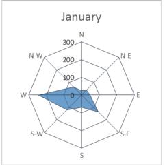
The month of July receives the maximum amount of radiation and we plotted a graph showing the radiation distribution in the various directions. It can be seen that the month of July receives higher amount of radiation in all the three predominant directions like East,South and West. The radiation in the South West and South East is higher than the South since they receive a higher amont of direct radiation than South.
Step 3 – Average Daily/Minimum and Maximum Temperature
The average daily temperature which is calculated as the mean average of the temperature variation along the 24 hours of each day.
Daily Temperature
-10.00 -5.00 0.00 5.00 10.00 15.00 20.00 25.00 30.00 1 13 25 37 49 61 73 85 97 109 121 133 145 157 169 181 193 205 217 229 241 253 265 277 289 301 313 325 337 349 361 Temperature[ ° C] Days
Average
0.00 1.00 2.00 3.00 4.00 N N-E E S-E S S-W W N-W July
The maximum and mimimum daily temperature is calculated by taking the minimum and maximum values in the 24 hour interval for all the days of the year.
Minimum Daily Temperature
20.00
15.00
10.00
5.00
0.00
-5.00
25.00 1 13 25 37 49 61 73 85 97 109 121 133 145 157 169 181 193 205 217 229 241 253 265 277 289 301 313 325 337 349 361
Temperature[ ° C] Days
-10.00
Maximum Daily Temperature
30.00
25.00
20.00
15.00
10.00
5.00
0.00
35.00 1 13 25 37 49 61 73 85 97 109 121 133 145 157 169 181 193 205 217 229 241 253 265 277 289 301 313 325 337 349 361
Temperature[ ° C] Days
-5.00
The average daily temperature graph shows that during the Spring and Auntum there is a higher temperature variation within in a short span of days.
It can be seen even more clear from the graph of minimum and maximum daily temperature, especially during the march and september the minimum and maximum temperature for the consective days changes drastically.
Average annual minimum Temperature:
The average annual minimum Temperature or the coldest day of the year has a value of -3.67 °C which occurs on January 15 and is calculated by taking the minimum value of mean average daily temperature.
Monthly average values of Average daily,Minimum and Maximum daily temperature:
20.00
15.00
10.00
25.00 Temperature [ ° C]
5.00
0.00
Months
Maximum Monthly Temperature
15.00
10.00
5.00
0.00
Minimum Monthly Temperature 0.00 5.00 10.00 15.00 20.00 25.00 30.00 Temperature [ ° C]

Average Monthly Temperature -5.00
20.00 Months
Months
The minimum and maximum monthly teperature shows that during the period of Winter there is higher temperature variation on the same months than the period of summer when the temperature variation is comparitively low.
Step 4 – Comparison of Radiation and Temperature of hottest day
We can see from the calculated average daily temperature values that the hottest summer day of the year is the 8th July which receives a peak maximum temperature of 32.05 °C at the 17th hour of the day. The average temperature of the day is 26.49 °C.
Summer extreme day - 8th July
35.00
30.00
25.00
20.00
15.00
10.00
5.00
0.00
Temperature [ ° C] hours
1 2 3 4 5 6 7 8 9 10 11 12 13 14 15 16 17 18 19 20 21 22 23 24
TRNSYS UNI 10349
In the summer extreme day comparison between UNI and TRNSYS we can see that even thought the trend of the variation is similar but the Peak temperature of the day has shifted from 17.00 hour to 13.00 hour.
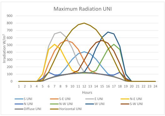
Comparison of day with maximum Irradiation - 29th July – Total Radiation recieved [38.56 KWh/m2]
The Value for the maximum radiation from TRNSYS is done by calculating the total sum of radiation from all the directions and by choosing the day with the maximum sum of radiation from all the directions.
The dffuse radiation from the TRNSYS is taken from the North direction since it has the minimum value of diffuse radiation.
Even though 8th of July being the hottest day with the value of average daily temperature it receives lesser total radiation of 30.21 KWh/m2 from all the faces than 29th July which has the average day temperature of 20.40 °C and receives a total radiation of 38.56 KWh/m2 .
800
700
600
500
400
300
200
100
900 1 2 3 4 5 6 7 8 9 10 11 12 13 14 15 16 17 18 19 20 21 22 23 24
Irradiation W/m 2 Hours
0
Maximum Radiation TRNSYS S TRNSYS S-E TRNSYS E TRNSYS N-E TRNSYS N TRNSYS N-W TRNSYS W TRNSYS S-W TRNSYS Diffuse TRNSYS
The graph shows that apart from higher value of radiation in TRNSYS than UNI, the Radiation is maximum for the East and in the early hour of the day and the west direction has its Peak value at the later hour of the day and the same concept is applicable to all the other directions. It is also seen that the radiation for the all the directions never go below the minimum diffuse radiation curve since it is because even though the direction loses the direct radiation it still receives the diffuse radiation.
Maximum Radiation UNI S UNI S-E UNI E UNI N-E UNI N UNI N-W UNI W UNI S-W UNI Diffuse UNI Horizontal UNI 0.00 200.00 400.00 600.00 800.00 1000.00 1 2 3 4 5 6 7 8 9 10 11 12 13 14 15 16 17 18 19 20 21 22 23 24 Irradiation [W/m 2 ] Hours
South - 29th July
South East - 29th July
0 100 200 300 400 500 600
Irradiation [W/m 2 Hours
1 3 5 7 9 11 13 15 17 19 21 23
800
600
400
200
0
Irradiation [W/m2] Hours
1 3 5 7 9 11 13 15 17 19 21 23
South UNI South TRNSYS
North East - 29th July
150
100
50
Irradiation [W/m2] Hours
200 1 3 5 7 9 11 13 15 17 19 21 23
0
800
600
400
200
1000 1 3 5 7 9 11 13 15 17 19 21 23
Irradiation [W/m2] Hours
0 100 200 300 400 500 600 1 3 5 7 9 11 13 15 17 19 21 23
Irradiation [W/m2] Hours
North East UNI North East TRNSYS
East - 29th July
South East UNI South East TRNSYS 0
North - 29th July North UNI North TRNSYS 0 100 200 300 400 500 600 700 1 3 5 7 9 11 13 15 17 19 21 23
North West - 29th July
Irradiation [W/m2] Hours
East UNI East TRNSYS
West - 29th July
Irradiation [W/m2] Hours
North West UNI North West TRNSYS 0 200 400 600 800 1000
1 3 5 7 9 11 13 15 17 19 21 23
West UNI West TRNSYS
South West - 29th July
0 200 400 600 800 1 3 5 7 9 11 13 15 17 19 21 23
Irradiation [W/m2] Hours
South West UNI South West TRNSYS
0 50 100 150 200
Diffuse North - 29th July
Irradiation [W/m2] Hours
1 3 5 7 9 11 13 15 17 19 21 23
Diffuse UNI Diffuse North TRNSYS
Step 5 –
Horizontal - 29th July
1000 1 3 5 7 9 11 13 15 17 19 21 23
500
0
Irradiation [W/m2] Hours
Horizontal UNI Horizontal TRNSYS
Comparison of average wind velocity:
Monthly frequency (time/month) of Wind with respect to directions


Yearly frequency of wind
The monthly frequency of wind direction shows thar each month has a predominant direction when the frequency is higher and it varies with each month and also it can be seen that the frequency from North is very low, this can be due to a potention barrier of wind like mountains in the North.


The Yearly frequency illustrates that West,South-West/South-East,South is the direction with maximum frequency of wind while North being the least.

Monthly Maximum Wind Velocity
Maximum wind velocities
This graph justifies the fact that we illustrated in the previous point from the fact that the S-E,S-W,S are the directions where we have the maximum wind velocities while we have the month of January and March when ther is the maximum wind velocity from the North and East direction.
Monthly average wind velocity [m/s] with respect to direction

0 2 4 6 8 10 12 14 16 N S-E E S-E W N-W S-W S-W S S W S January February March April May June July August September October November December VELOCITY [M/S] MONTH
The average wind velocity is quite same in all the directionand it is also higher in the North compared to the other values.
It can also be seen from the annual average wind velocity below that we have the average wind velocity which is equal in all the directions.


Yearly Average wind velocity The monthly average wind velocity comparison between TRNSYS and UNI shows that the values differs each month while the UNI has a higher average wind velocity in some months and the TRNSYS has a higher value in some months. But the difference in margin between the two values are lower.
Monthly average wind velocity UNI 10349 TRNSYS
0 1 2 3 4 N N-E E S-E S S-W W N-W Year
0.0 0.5 1.0 1.5 2.0 2.5 3.0 VELOCITY [M/S] MONTH
Step 6 – Horly average values of the temperature and RH :
Average hourly temperatures
Average hourly relative humidity
January February March April May June July August September October November December
January February March April May June July August September October November December
The relative humidity decreases as the temperature increases in successive hours of the day. The temperature variation (ΔT) in a single day is higher in the period of Autumn and Spring. The pick of temperature is traslating some hours after moving from winter to summer.
5 10 15 20 25 30
-5 0
1 2 3 4 5 6 7 8 9 10 11 12 13 14 15 16 17 18 19 20 21 22 23 24 Temperature [ ° C] hour
50 55 60 65 70 75 80 85 90 95 100
1 2 3 4 5 6 7 8 9 10 11 12 13 14 15 16 17 18 19 20 21 22 23 24 RH [%] Hours
Step 9 – Analysis with different weather data files :
The follwing graphs illustrates the comparison of all the main characterstics with different data files:
1 – Milano Linate - epw
2 – Milano Malpensa – epw
3 – Milano Malpensa – tmy2
4 – Milano – epw
5 – Milano – cti
6 – Milano Linate – tmy2 0.00 10.00 20.00 30.00 40.00 50.00 60.00 70.00 80.00 90.00 100.00
Comparison monthly horizontal total radiation 1 2 3 4 5 6
0.00 1.00 2.00 3.00 4.00 5.00 6.00 7.00 8.00 kWh/m 2 Month
Comparison monthly average relative humidity 1 2 3 4 5 6
RH (%) Month
25.00
20.00
15.00
10.00
5.00
0.00
-5.00
Climate data – Milano Malpensa.tmy2
Horizontal Radiation UNI
Comparison monthly average temperatures 1 2 3 4 5 0 1 2 3 4 5 6
30.00 T (°C) Month
IT_H-UNI IB_H-UNI ID_H-UNI
Horizontal Radiation TRNSYS
IT_H-TRNSYS IB_H-TRNSYS ID_H-TRNSYS 0 1 2 3 4 5 6 7


Climate data – Milano Malpensa.epw


All the other graphs are shown in the respecticve excel files for the verification.
Number of hours
above
30.00
25.00
20.00
15.00
10.00
temperatures Night temperat ure - 19 to 7 Day temperat ure - 7 to 19

5.00
Step 10 – Important datas : -10.00
35.00 0 500 1000 1500 2000 2500 3000 3500 4000 4500 5000
0.00
-5.00
T ( ° C) Hour
Course of Building Energy Modelling Report Exercise 2 – Thermal Zone Analysis Group 6 Andrea Battistel 854584 08/05/2016 Velmurugan Siva Kamaraj 854328
Introduction:
In this Exercise we took an ideal thermal zone and performed 21 different types of analysis by varying its parameters and boundary conditions. We perform the analysis first by creating a geometrical model in sketchup and then followed by the thermal analysis in TRNbuild.
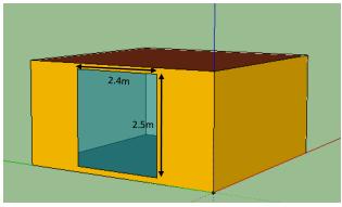
Ideal Thermal Zone
2.8m 2.5m
Ideal Thermal Zone with Window in the West Facade


In the above thermal zone we introduced a window of dimension 2.4m X 2.5m in the West Facade.

In the same thermal Zone we intoduce the shaded window. In order to do so, a shading group has been created with the shading element that has the same dimension of the windows and it has been placed at a distance of 0.5m from the window.

Thermal Zone / Material Characterstics
The thermophysical characteristics of the walls, ceiling and floor are given in the following table. The layers are described in order from external to internal. d [m] λ [W/(mK)] r [kg/m3] cp [kJ/(kgK)] [kJ/(kgK)]
Type 1 (external wall)
Outer layer 0.115 0.99 1800 0.85 Insulating layer 0.06 0.04 30 0.85 Masonry 0.175 0.79 1600 0.85
Internal plastering 0.015 0.7 1400 0.85
Type 2 (internal wall)
Gypsum plaster 0.012 0.21 900 0.85 Mineral wool 0.1 0.04 30 0.85 Gypsum plaster 0.012 0.21 900 0.85
Type 3c (ceiling)
Plastic covering 0.004 0.23 1500 1.5 Cement floor 0.06 1.4 2000 0.85
Mineral wool 0.04 0.04 50 0.85 Concrete 0.18 2.1 2400 0.85
Type 3f (floor)
Concrete 0.18 2.1 2400 0.85 Mineral wool 0.04 0.04 50 0.85 Cement floor 0.06 1.4 2000 0.85
Plastic covering 0.004 0.23 1500 1.5
Type 4c (ceiling/roof)
Plastic covering 0.004 0.23 1500 1.5 Cement floor 0.06 1.4 2000 0.85
Mineral wool 0.04 0.04 50 0.85 Concrete 0.18 2.1 2400 0.85 Mineral wool 0.1 0.04 50 0.85 Acoustic board 0.02 0.06 400 0.84
Ideal Thermal Zone with Shaded Window in the West Facade
Type 4f (floor)
Acoustic board
0.02 0.06 400 0.84
Mineral wool 0.1 0.04 50 0.85 Concrete 0.18 2.1 2400 0.85
Mineral wool 0.04 0.04 50 0.85 Cement floor 0.06 1.4 2000 0.85 Plastic covering 0.004 0.23 1500 1.5
Type 5 (roof)
Rain protection 0.004 0.23 1500 1.3 Insulating 0.08 0.04 50 0.85 concrete 0.2 2.1 2400 0.85
Thermal Zone / Windows and Shading Component Characterstics
Type of Window – Double Pane 4/16/4 - Trnbuild Window Lib Id – 1202


Thermal transmittance of the glazing system - Ug 2.83 W/(m2 K) Thermal transmittance of the frame - Uf 2 W/(m2 K)
Total solar energy transmittance of the glazing system - g_glass 0.75Total solar energy transmittance of the window system - g_window 0.23Percent Area of Glass over Window 18 %
Shading Factor 0.693 -
Legal Hour Correction (hours)
Since the Schedules for the different aspects are given in legal time, we implemented the legal hour correction in the schedules. These regards to the Internal Gains, Ventilation, Heating and Cooling System.
0 1995 2520 6889 7203 8760
Hours
Heating Season
Cooling Season
Legal Hour Correction (*Summer) - Schedule 7_17hours (Workdays)
Legal Hour Correction (*Winter) – Schedule 8_18hours (Workdays)
Schedules used in TRNSYS are as follows:
Schedule 8_18 – This Schedule allows the system to be ON from 08:00 to 18:00 during Weekdays and OFF during other hours and keeps the system completely OFF during Weekends.
Schedule 7_17 – This Schedule allows the system to be ON from 07:00 to 17:00 during Weekdays and OFF during other hours and keeps the system completely OFF during Weekends. This Schedule is introduced in the Exercise in order to follow the Schedules according to the legal hour Correction; (Note: The time schedules for all tests are given in legal time, which is 1 h ahead of solar time in summer).
Schedule Always ON – This Schedule allows the system to be ON during all the hours of the Weekdays and Weekends.
The setpoint temperature for the Heating System is 26°C while for the Cooling System it is 26°C.
Tests:
As mentioned above we have three types of thermal zones from which we have carried out 21 different analysis by either changing the materials or by changing the system characterstics. We used milano-linate.tmy2 as the weather data file.
Outputs to be controlled are:
For tests 1 to 3: internal air temperatures (monthly average values), monthly and seasonal frequency charts, daily internal air temp (21th December, 21th June).
For tests 4 to 7: energy needs (expressed in kWh) for heating (QH) and cooling(QC), given on monthly basis and for the whole year. the hourly pattern of the calculated internal temperatures(focusing on the beginning and the end of the cooling season)
For test 8 to 20: energy needs (expressed in kWh) for heating (QH) and cooling(QC), given on monthly basis and for the whole year;the hourly pattern of the calculated internal temperatures(focusing on the beginning and the end of the cooling season and on the night temperatures).
The results for the different tests have been produced in terms of graphs and comparison charts which are as follows.
Test 1:
Test External wall Glazing system
1
Adiabatic internal vertical wall Adiabatic ceiling Adiabatic floor
Type 1 None Type 2 Type 4c Type 4f
Internal Gains 20W/m2 and Free Floating Schedule 7_17 - 1995 to 7203 hours / Schedule 8_18 - 7203 to 1995 hours
The building behaves like a closed box with just one surface exposed to the outside and so the we can see the average temperature higher than 20°C all over the year, reaching almost 50°C during the summer.

Monthly Frequency Charts


During the cold period the temperature is lower than 20°C just for a few hours (in January and February)
During the hot period the temperature is never below 36 °C.
Seasonal and yearly Frequency Charts

Autumn has a larger frequency of the higher temperature with respect to the spring period (i.e. range from 42 to 44°C has high frequency in Autumn than Spring).

The range of temperature with the high frequency throughout the year is (42-46)°C. The reason for these values is that the building is in contact with the outside just through one surface (without the window) and so the heat dispersion are very low.

Internal Air Temperature 21st December and 21st June
The hourly temperature during these two days is obiouvsly different but it’s very clear that they follow the same shape. In particular there is a strong variation in the trend of the curves during the 8 and 18 hour, when the internal gains starts and stops.

Test External wall Glazing system
2
Adiabatic internal vertical wall Adiabatic ceiling Adiabatic floor
Type 1 DP Type 2 Type 4c Type 4f
Ventilation - 1 Volume/hour, Internal Gains 20W/m2 and Free Floating Schedule 7_17 - 1995 to 7203 hours / Schedule 8_18 - 7203 to 1995 hours
The monthly average temperature goes down to 10 °C during the winter period, while during the summer it’s higher than 40°C.

Monthly Frequency Charts

Test 2:

In September the frequency of temperature ranges are very similar since the temperature varies a lot during this period.
Seasonal and yearly Frequency Charts


During winter and summer it’s easy to find the range with the maximum frequency, while during spring and autumn there are more different range of temperatures with a similar frequency.
The range with the maximum frequency is (42-46) °C since we have a similar situation like in test but with the presence of the window.
The trend of the two curves are again similar; this time at 8 and 18 hour there is just a small variation of the shape because the ventilation and internal gain starts during the same hour.

 Internal Air Temperature 21st December and 21st June
3
Type 1 Shaded DP Type 2 Type 4c Type 4f Ventilation - 1 Volume/hour, Internal Gains 20W/m2 and Free Floating Schedule 7_17 - 1995 to 7203 hours / Schedule 8_18 - 7203 to 1995 hours
The monthly avarage temperature stay around 10°C during the winter period and reach 30°C during the summer period

Monthly Frequency Charts

Test 3: Test External wall Glazing system Adiabatic internal vertical wall Adiabatic ceiling Adiabatic floor

During January and February the temperure is quite stable around a specific range of temperature (6-10°C) while during August and July we have the same situation but with different range (28-30)°C.

Seasonal Frequency Charts
Again in the test 3 there is a strong frequency of some specific range during winter and summer, while during spring and autumn the temperature is more variable.

The range with the maximum frequency is 26-30 °C
The trend of the two curves is again similar, but the shape regarding 21st December is less affected by the start and the end of the interal gain and ventilation period. So using the shading system the daily thermal excursion is lower, maybe because the incident radiation on the window is much low.

 Internal Air Temperature 21st December and 21st June
The monthly average temperature of test 2 is lower than test 1 particularly during the spring and autumn because the natural ventilation bring fresh air from the outside; the temperature of test 3 is strongly lower during summer because the shading reduce the heat gain by the sun.


The presence of the window and the ventilation bring the test 2 and 3 to a lower hourly temperature, while the difference is higher especially during winter period.

The frequency chart shows that the test 3 reach the minimum temperature during winter because again the shading reduce the heat gain by the sun; the test 1 reaches the maximum temperature during summer because there is no ventilation.

Comparison graphs test 1-2-3
When we introduced shading in the thermal zone we create the shading element in sketchup and gave the external shading factor as 0.693. But we realize that in this case the program considers the shading element two times, considering both an opaque element in front of the window and also reducing the g value of the shaded window. So we repeated the test 3 by not creating a shading element in the sketchup and by giving the integrated shading facto as 0.693. By doing so we found the the monthly average temperature varying largely; so we corrected this mistake for the test 21 since we finished doing all the tests in the same procedure that is mentioned earlier.
It’s cleary visible from the graph that the case with the shading group in sketch up as well as with an external shading factor equal to 0,693 gives very similar temperature to the case with no shading in sketch up but external shading factor equal to 1 ( meaning no solar gain). This means that in our simulation the heat gain calculated are lower than the real one.

Test 3B
4
Type 1 Shaded DP Type 2 Type 4c Type 4f
Ventilation - 1 Volume/hour, Internal Gains 20W/m2 and Heating and Cooling Continous
Schedule 7_17 - 1995 to 7203 hours / Schedule 8_18 - 7203 to 1995 hours/schedule always ON (heating and cooling)
The Cooling energy need is much lower than the heating energy need, since the temperature must be cooled down just for few degrees (i.e. to set point temperature 26°C) during summer. This is due to the fact that the average monthly temperature of the thermal zone without the cooling system is around 30°C (as shown in the third case).


Test 4:
Test External wall Glazing system Adiabatic internal vertical wall Adiabatic ceiling Adiabatic floor
It can be seen from the Winter hourly temperature graph that the heating system is always on because the temperature is never below 20°C; during the middle of the day the temperature is generally higher than 20°C, meaning that the heating system is not needed.

From the summer hourly average temperature it is seen that in most of the hours there is no need of cooling since the average temperature is lower than the set point temperature (26°C)
The hourly pattern shows that the minimum night temperature, both during the beginning and the end of the cooling season, is around 18°C.

Test External wall
Glazing system Adiabatic internal vertical wall Adiabatic ceiling Adiabatic floor Type 1 Shaded DP Type 2 Type 3c Type 3f 5 Ventilation - 1 Volume/hour, Internal Gains 20W/m2 and Heating and Cooling Continous Schedule 7_17 - 1995 to 7203 hours / Schedule 8_18 - 7203 to 1995 hours/schedule always ON (heating and cooling)
The trend of the monthly energy consumption are very similar to the ones of the test 4.


Test 5:
Between the 2 tests there is anyway a small difference in the total consumption all over the year, because here the wall has an higher thermal inertia due to the position of the massive layer (concrete). For example if this layer is put in the internal position (like type 3c), it’s allowed to embody a lot of energy coming from the internal gain and the heating system (that is continous): the heat flux going outside will take more time and the consequence is the reduction of the energy need to heat the zone. year Qcool (kWh) Qheat (kWh) TEST 4 292 1055 TEST 5 274 1045
During the summer the average temperature is below 26°C and this is the reason why the energy need for heating is much higher than the energy need for cooling (like in test 4).

Because of the increased thermal inertia we have also a little higher minumum temperature during the night in the same period with respect to the test 4 (19 °C against 18°C).

Test External wall Glazing system
Adiabatic internal vertical wall Adiabatic ceiling Adiabatic floor
Type 1 Shaded DP Type 2 Type 4c Type 4f
6 Ventilation - 1 Volume/hour and Heating and Cooling Continous Schedule 7_17 - 1995 to 7203 hours / Schedule 8_18 - 7203 to 1995 hours/schedule always ON (heating and cooling)
The coolind energy demand is very close to zero, because of the absence of the internal gain, and more in our simulation we have a very low amount of heat gain by the sun (due to the method to model the shading system). As opposite the heating energy consumption is very high.


Test 6:
The average hourly temperature during winter is usally near to 20°C, meaning that the heating system is always working; during the summer the hourly average temperature is below 21°C.

The hourly pattern shows that during the transition period between heating and cooling the temperature reach 26°C just for some hours, confirming that the cooling system is not needed so much.


Test 7:
Test External wall Glazing system Adiabatic internal vertical wall Adiabatic ceiling Adiabatic floor Type 1 DP Type 2 Type 4c Type 4f 7 Ventilation - 1 Volume/hour, Internal Gains 20W/m2 and Heating and Cooling Continous Schedule 7_17 - 1995 to 7203 hours / Schedule 8_18 - 7203 to 1995 hours/schedule always ON (heating and cooling) year Qcool (kWh) Qheat (kWh) TEST 4 292 1055 TEST 7 1588 733
The test 7 is not provided by the shading system and this is visible in the energy consumption; the presence of the solar irradiance without any control increases a lot the energy demand for cooling while decrease at the same time the energy demand for heating. The sum of both value shows that the situation with shading reduce yearly energy consumption.
Because of the solar irradiance the winter average temperature during the middle of the day is higher than 20°C, so the heating system is not needed during these hours.
During the summer the hourly average temperature goes much down from 26°C just during the night. So we can say that without the shading system the internal temperature is strongly influenced by the sun radiation.

The hourly pattern shows that when starts the cooling season, the system has to work almost every day from the middle of april.

The energy demand for cooling is much higher for the test 7 with respect to all the other test, saying that the solar radiation has a really strong role.
For the heating energy demand the test 6 is the worst one, because all the free heat coming from internal gain has to be provided here by the heating system.

Comparing the total yearly energy demand, the test 5 (with the increased thermal inertia) has the best result, for the same reason explained before.

Comparison graphs test 4-5-6-7
The Cooling energy need is similar to the one of the test 4 eventhough the system is working just for 10 hours since the system is off during the night when the temperature is below our set point temperature.

The heating energy need is lower than the one of the test 4 because the system is off during the critical period (night) when the temperature is below our setpoint temperature while the test 4 works continously.

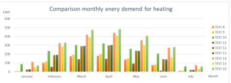
Test 8:
External wall Glazing system Adiabatic internal vertical wall Adiabatic ceiling Adiabatic floor Type
Type
Type
Type
Qcool (kWh) Qheat (kWh)
Test
1 Shaded DP
2
4c
4f 8 Ventilation - 1 Volume/hour, Internal Gains 20W/m2 and Intermittent Heating and Cooling Schedule 7_17 - 1995 to 7203 hours / Schedule 8_18 - 7203 to 1995 hours
290.59 691.37
The winter hourly temperature clearly shows us that the zone temperature is maintained during the working hours of the system while it is very low during the other hours which is the main reason for the lower heating energy need than test4.

The same is the case for the Summer hourly temperature and cooling energy need.
The hourly pattern illustrates the working condition of our heating and cooling system (the weekend temperature is very low than setpoint temperature during winter and viceversa for summer)


Test 9: Test External wall Glazing system Adiabatic internal vertical wall Adiabatic ceiling Adiabatic floor
Qcool (kWh) Qheat (kWh) 273.34
9 Type 1 Shaded DP Type 2 Type 3c Type 3f Ventilation - 1 Volume/hour, Internal Gains 20W/m2 and Intermittent Heating and Cooling Schedule 7_17 - 1995 to 7203 hours / Schedule 8_18 - 7203 to 1995 hours The cooling energy need is lower than test 8 since the wall has higher conductivity which makes it more resistance against cooling.
The heating need is higher than the test 8
768.01
The Winter hourly temperature is near to 20°C during the working hours of the system while it is low during the other hours.


The temperature during the weekend is very low since we do not have gains and due to the absence of cooling system.
It also shows that during the beggining of the season the full working condition of the system during its working hours since it the temperature is very low while at the end of the season it works even less since the temperature is lower.
10
Type 1 Shaded DP Type 2 Type 4c Type 4f Ventilation - 1 Volume/hour and Intermittent Heating and Cooling Schedule 7_17 - 1995 to 7203 hours / Schedule 8_18 - 7203 to 1995 hours
Qcool (kWh) Qheat (kWh) 1.14 1472.28


The heating energy need is higher that the test 9 since we do not have an internal gain which leaves the zone with low temperature making the increase in the heating energy need.
The cooling energy need is lower since we are losing the gain which leaves the temperature lower makinng the decrease in the cooling energy need.
Test
10: Test External wall Glazing system Adiabatic internal vertical wall Adiabatic ceiling Adiabatic floor
The above graph shows us that cooling sytem is not working in most of the hours of its working period since during most of the times we are in higher temperature that 26°C.

During the end of the season it starts to work even less as the temperature is even more low.


Test 11: Test External wall Glazing system Adiabatic internal vertical wall Adiabatic ceiling Adiabatic floor 11 Type
Qcool
Q
1 DP Type 2 Type 4c Type 4f Ventilation - 1 Volume/hour, Internal Gains 20W/m2 and Heating and Cooling Continous Schedule 7_17 - 1995 to 7203 hours / Schedule 8_18 - 7203 to 1995 hours The cooling energy need is very high because of the absence of solar protection which results in higher solar gain. The heating energy need is lower for the same reason. The values of the heating and cooling need is lower than test 7 because of the number of working hours is lower in the test 11.
(kWh)
heat (kWh) 1335.35 454.10
The winter hourly temperature is maintained as 20°C during its working hours while it is not that low even during the absence of gains because of the increased solar gain due the absence of solar protection.

The above graph shows that the cooling system has to work a lot since we have higher temperature in the zone exceeding our set point temperature.

12
Type 1 Shaded DP Type 2 Type 5 Type 4f Ventilation - 1 Volume/hour, Internal Gains 20W/m2 and Intermittent Heating and Cooling Schedule 7_17 - 1995 to 7203 hours / Schedule 8_18 - 7203 to 1995 hours
The heating energy need is higher than test8 since we have an external roof that is exposed to the outdoor which decreases the temperature of the zone during the nonworking hours of the system.
The cooling energy need is similar to test8 since the system is off during the night when the temperature is lower so even in the case with heating and cooling system working continuous they tend to be off because of the lower temperature.


Test 12:
Test External wall Glazing system Adiabatic internal vertical wall External Roof Adiabatic floor
Q
Qcool (kWh)
heat (kWh) 319.57 1203.11
The average hourly temperature is lower due to the presence of external roof which allows the heat flow.


1 Shaded DP
2 Type 5 Type 3f Ventilation - 1 Volume/hour, Internal Gains 20W/m2 and Intermittent Heating and Cooling Schedule 7_17 - 1995 to 7203 hours / Schedule 8_18 - 7203 to 1995 hours We can see that the cooling and heating energy need is very much similar to the one of test 12 since they both differs just with the material. The change in the values are due to the difference in the thermal resistance of the building; in this case the higher thermal inertia has a negative result because in this case we have a intermittant heating and cooling system.


Test 13: Test External wall Glazing system Adiabatic internal vertical wall External Roof Adiabatic floor
13 Type
Type
Qcool (kWh) Qheat (kWh) 323.11 1212.57


14 Type 1 Shaded DP Type 2 Type 5 Type 4f Ventilation - 1 Volume/hour and Intermittent Heating and Cooling Schedule 7_17 - 1995 to 7203 hours / Schedule 8_18 - 7203 to 1995 hours
The cooling energy need is lower since we have the absence of internal gains which makes the zone temperature lower making the cooling system to remain off during most of the time.

The heating energy need is very high on the contrary since the absence of gains makes the temperature even more low during winter making the heating system to work in order to achieve the set point temperature,

Test
Test
Glazing
Adiabatic
14:
External wall
system
internal vertical wall External Roof Adiabatic floor
Qcool (kWh) Qheat (kWh)
15.03 2005.21
The above graph shows that the hourly pattern of the temperature is lower than 26°C during most hours making the cooling system almost switched off.


0 50 100 150 200 250 300 350 400 450 kWh Month
Type 1 DP Type 2 Type 5 Type 4f Ventilation - 1 Volume/hour, Internal Gains 20W/m2 and Heating and Cooling Intermittent Schedule 7_17 - 1995 to 7203 hours / Schedule 8_18 - 7203 to 1995 hours The Cooling energy need is higher than the one of test 14 due to the absence of solar protection which increases the temperature of the room The same case for heating energy demand becasue of the absence of solar protection and the presence of external roof makes it even more open to the environment increasing the energy demand.
Monthly energy consumption Qcool (kWh) Qheat (kWh)

Test 15: Test External
Glazing
Adiabatic
External
Adiabatic floor
wall
system
internal vertical wall
Roof
15
Qcool (kWh) Qheat (kWh) 590.95 1638.14


Test 16: Test External wall Glazing system Adiabatic internal vertical wall External Roof Adiabatic floor 16 Type 1 Shaded DP Type 2 Type 5 Type 4f All Exposed Surfaces Ventilation - 1 Volume/hour, Internal Gains 20W/m2 and Intermittent Heating and Cooling Schedule 7_17 - 1995 to 7203 hours / Schedule 8_18 - 7203 to 1995 hours
The hourly pattern shows that the during the beginning and the end of the season the temperature is lower than the setpoint temperature making the cooling system work less.
The high value of heating energy demand is due to the fact that since the zone envelope is exposed to outdoors in all the surfaces,the heat loss increases making the energy demand increase even more.


the test 11 is the worst as for the cooling energy demand because there is no solar control


The test 16 is the worst regarding the heating energy demand because all the surfaces are exposed to the outside.

Comparison 8 to 16
Test External wall Glazing system
17
Adiabatic internal vertical wall Adiabatic ceiling Adiabatic floor
Type 1 Shaded DP Type 2 Type 4c Type 4f
Thermal Bridges
Ventilation - 1 Volume/hour and Internal Gains 20W/m2 Intermittent Heating and Cooling Schedule 7_17 - 1995 to 7203 hours / Schedule 8_18 - 7203 to 1995 hours
For the test 17 we start with the test 8 but we consider also the thermal bridges; the procedure follow the simplificative method, in which we take the values of the linear trasmittance by the UNI 14683 - 2008. This values are used to modify the thermal trasmittance of the wall and the roof, that are the only surfaces in contact with the outside, in order to have a more realistic model; until now we design the building using interior dimension, so we use this value also for the psi.


Once we calculated the new thermal trasmittance, on TRNSYS we modify the conductivity of the insulating layer to reach the real value of the U.
WALL code ψ l ψ*l (ψ*l)/A Uwall old Uwall new thermal bridge W/ m K m W/K W/m2 K W/m2 K W/m2 K window/wall W7 0.45 9.80 4.41 pillar P1 1.30 2.80 3.64 intermidiate floor (1/2) IF1 0.10 5.50 0.28 corner wall/roof (1/2) R1 0.75 5.50 2.06 total 10.39 1.11 0.490 1.595 ROOF corner wall/roof (1/2) R1 0.75 5.50 2.06 0.07 0.241 0.248
W7: material thermal bridge between window and the wall with external insulation P1: material thermal bridge in the correspondance of the pillar IF1: geometrical thermal bridge between intermediate floor and the wall R1: geometrical thermal bridge in the corner of two wall with external insulation

Test 17:
year Qcool (kWh) Qheat (kWh)


TEST 8 291 691
TEST 17 254.01 1018
The result shows that the presence of the thermal bridge increase a lot the energy need for the heating and decrease the one for the cooling.
During the winter the higher value of the thermal trasmittance of the external wall increases the heat flow to the outside, causing a higher demand of energy to keep the internal air temperature at 20°C.
During the summer the thermal bridges may have a positive result, because increasing the exchange of heat between inside and outside, during the night the air temperature is naturally cooled down and the demand for cooling system is lower.
During the beginning of the cooling season the night air temperature is low, reaching also 16°C.

Test External wall
Glazing system Adiabatic internal vertical wall External Roof Adiabatic floor Type 1 Shaded DP Type 2 Type 5 Type 4f 18 Floor on Groud (Tground Average = 11°C) Ventilation - 1 Volume/hour and Internal Gains 20W/m2 Intermittent Heating and Cooling Schedule 7_17 - 1995 to 7203 hours / Schedule 8_18 - 7203 to 1995 hours


Test 18:
year
cool (kWh) Q
In the test 18 the floor is in contact with the ground that a costant temperature equal to 11°C. For this reason there is a heat flow coming from the inside to the ground that influence the result: in the winter there is an increasing of the heating energy demand while during the summer there is a decreasing of the cooling demand. (kWh) TEST
Q
heat
8 291 691 TEST 18 29.85 1006
The summer average hourly graph shows that the temperature during the night goes down a lot, reaching almost 18°C.


In this test we provide a dynamic shading device that is closed when the radiation is higher than 300 W/mq during summer and higher than 200 W/mq during winter. In this way we allow radiation to enter during the heating season and the result is the decreasing of the heating energy demand. During the cooling season the energy need is higher because in the test 8 the shading system is always closed. The hourly pattern and the average seasonal temperature are quit similar to the one of test 8.


Test 19:
Test External wall Glazing system Adiabatic internal vertical wall External Roof Adiabatic floor Type 1 Shaded DP Type 2 Type 5 Type 4f 19
year Qcool (kWh) Qheat (kWh) TEST 8 291 691 TEST 19 428 619
Shading Control >200W/m2 for Heating Season and >300 W/m2 for Cooling Season Ventilation - 1 Volume/hour and Internal Gains 20W/m2 Intermittent Heating and Cooling Schedule 7_17 - 1995 to 7203 hours / Schedule 8_18 - 7203 to 1995 hours
Test 21:
We created three thermal zones in the sketchup, where two thermal zones having window in the western direction have the same properties as test 8 while there is an adjacent zone that has the properties of test1.
The shading for this test is given by not creating a shading group in the sketchup but by giving the integrated shading factor of 0.693.

Zone 2
Zone 1
Zone 3
The increase in the monthly average temperature of the Zone 3 is due to the fact that this zone does not have a window.
The temperature of this zone is comparitively lower than test 1 eventhough they both dont have the window since the zone 3 is exposed to the outdoors in the longer dimension of it which makes the heat flow higher than test1.

Test21 is the worst regarding both the heating and cooling because the area that has to be heated is higher.

Test18 is the best because of the position of the floor, as explained before.

Comparison 17 to 21
FINAL COMPARISON
As a final summary we plot a graph comparing all the result from test 4 to 21; the energy needs are divided by the are of the building. From this graph we can understand the worst and the best case between all: - worst cases are the test7 and 16: the solar protection and the exposure to the outside are so the main factor that affect our analysis. -best case is the test 8, because we have a fixed shading and the intermittant cooling and heating system.

Course of Building Energy Modelling Report Exercise 3 – Thermal Zone Analysis
Group 6
Andrea Battistel 854584 04/06/2016 Velmurugan Siva Kamaraj 854328
Table of Contents
1.Introduction
1.1 Citations of the Report
2.Symbols and Abbreviations
3.Description of fixed Parameters
4.Simulation Results
Aim and Objectives
4.1. Part 1 – Study of Thermal Inertia
4.2. Part 2 – Decrease Power Demand
4.3. Part 3 – Avoid Cooling System
4.4. Part 4 – Analysis of Internal Textile Shading device
5.Annexures
5.1. Annexure Part 1 – Study of Thermal Inertia
5.2. Annexure Part 2 – Decrease Power Demand
5.3. Annexure Part 3 – Avoid Cooling System
5.4. Annexure Part 4 – Analysis of Internal Textile Shading device
6.References and Calculations
1.INTRODUCTION
In this exercise it has been provided a building located in Milan with the fixed geometry while the construction and the system charateristics can be varied in order to understand it’s behaviour and achieve the energy efficient performance.
Simulation Tool – Trnsys 17 and TRNBuild

5 5
Area (m2) 160 80 36 36
Assumptions made: Type of Building – Office Building Surface Occupancy – Individual office type Number of Occupants – 10 People Nature of Work – Seated, Very light writing Appliances – Computer (10 Nos) and Artificial Lighting [Gains of the Appliances are assumed in the TRNBuild according to the Category which are explained later) Surface Category 1 boundary 2 external 3 external 4 external 5 external 6 external Surface location n. window Area (m2) Uw (W/m2 K) Uf (W/m2 K) g factor
3 2.89 3 0.789 6 3 3 2.89 3 0.789 Trasparent surfaces Orientation H_0_0 E_270_90 N_180_90 S_0_90 E_270_7 W_90_90 Opaque surfaces
161.25 100
1.1.Citations of the Report –Brief description of each contents of the report
The citation for each of the content has been provided here to understand the nature of the contents
Symbols and Abbrievations – Includes the abbrievations for the nomenclature that we have used in this report.
Fixed Parameters – Includes the fixed Paramets that has been used in all the simulations
Simulation Results – Includes the the inputs and simulation results for each parts assessing the behaviour of each cases that we have done and giving a final remarks for each simulation study.
Annexures – Includes the modelling assumptions, inputs, variables, simulation results, graphs for all the cases for the respective parts.
2.SYMBOLS AND ABBRIEVATIONS

3.DESCRIPTION OF FIXED PARAMETERS – Building Material Characterstic
WALL
Description s (m) R (m2 K/W) U (W/m2 K)
W_1 0.493
Outer layer 0.115 0.12
Insulating layer 0.06 1.50
Masonry 0.175 0.22
Internal plastering 0.015 0.02
W_1_a 0.490
Outer layer 0.115 0.12
Insulating layer 0.056 1.40 Masonry 0.25 0.32
Internal plastering 0.015 0.02
W_1_b 0.494
Outer layer 0.115 0.12
Insulating layer 0.049 1.23 Masonry 0.4 0.51
Internal plastering 0.015 0.02
W_1_e 0.234
Outer layer 0.115 0.12
Insulating layer 0.15 3.75 Masonry 0.175 0.22 Internal plastering 0.015 0.02
W_1_f 0.148
Outer layer 0.115 0.12
Insulating layer 0.25 6.25 Masonry 0.175 0.22
Internal plastering 0.015 0.02
Convective coefficient h (W/m2 K)
Inner Surface 3.05
Outer Surface 17.8
ROOF
Description s (m) R (m2 K/W) U (W/m2 K)
R_1 0.24
Acustic board 0.02 0.33
Mineral wool 0.1 2.50
Concrete 0.18 0.09
Mineral wool 0.04 1.00 Cement floor 0.06 0.04 Plastic covering 0.004 0.02
R_1_a 0.24
Acustic board 0.02 0.33
Mineral wool 0.1 2.50 Concrete 0.3 0.14 Mineral wool 0.038 0.95
Cement floor 0.06 0.04 Plastic covering 0.004 0.02
R_1_b 0.24
Acustic board 0.02 0.33
Mineral wool 0.1 2.50 Concrete 0.35 0.17 Mineral wool 0.037 0.93 Cement floor 0.06 0.04 Plastic covering 0.004 0.02
R_1_e 0.185
Acustic board 0.02 0.33
Mineral wool 0.15 3.75 Concrete 0.18 0.09 Mineral wool 0.04 1.00
Cement floor 0.06 0.04
Plastic covering 0.004 0.02
R_1_e 0.145
Acustic board 0.02 0.33
Mineral wool 0.15 3.75 Concrete 0.18 0.09 Mineral wool 0.1 2.50
Cement floor 0.06 0.04 Plastic covering 0.004 0.02
GROUND FLOOR
Description s (m) R (m2 K/W) U (W/m2 K)
G_1 0.47
Rain protection 0.004 0.02
Insulating layer 0.08 2.00 Concrete 0.2 0.10
G_1_e 0.25
Rain protection 0.004 0.02
Insulating layer 0.15 3.75 Concrete 0.2 0.10
G_1_f 0.19
Rain protection 0.004 0.02 Insulating layer 0.2 5.00 Concrete 0.2 0.10
WINDOW
Description Uw (W/m2 K) Uf (W/m2 K) g factor
Win_1 2.89 3 0.789 Win_2 1.43 2 0.605 Win_3 0.52 1 0.585
Materials λ (W/m K) δ (kg/m3) cp (kJ/kg K)
Outer layer 0.99 1800 0.85
Insulating layer 0.04 30 0.85 Masonry 0.79 1600 0.85
Internal plastering 0.7 1400 0.85
Acustic board 0.06 400 0.84
Mineral wool 0.04 50 0.85 Concrete 2.1 2400 0.85
Cement floor 1.4 2000 0.85
Plastic covering 0.23 1500 1.5
Rain protection 0.23 1500 1.3 Insulating layer 0.04 50 0.85
Building System Characterstics
Air exchange by standard
Standards: UNI 11300 and UNI 10339
Description Value Units
nper,k 10qve,o,p,k 0.011 m 3/s qve,o,s,k 0ns,k 0.06 people/m2 Af,k 160 m 2 eve,c 0.8C1 1C2 1qve,o 396 m 3/h Volume 720 m 3 n 0.55 vol/h
Air exchange by hygenic reson
Description Value Units


qvep 30 m 3/h person nper,k 10qve 300 m3/h n 0.42 vol/h
Ventilation AE (vol/h) reference
Standard 0.55 standard Hygenic 0.42 hygenic value Night vent 1 assumption
Heating and Cooling systems
Description Set point temperature (°C) Day range Hour range
Heating system
20
15 Oct - 15 April 0 - 2520 / 6889 - 7860
Cooling system 26 15 April - 15 Oct 2520 - 6889
Internal gains
Schedules
Name Range (hr) Days
Intermittent 8.00 - 18.00 Monday - Friday Continous 0.00 - 24.00 All Continous Workday 0.00 - 24.00 Monday - Friday Night 18.00-8.00 All Worklight 8.00 - 18.00 Monday - Friday
4.SIMULATION RESULTS
Aims and Objectives:
4.1.Part 1 – Study of Thermal Inertia – To demonstrate the Positive aspects in the energy demand with the change of Thermal inertia of the building envelope.
4.2.Part 2 – Decrease Power Demand – To assess the strategies in order to have the maximum power demand lower than 20W/m2 and the Air Chnage rate of the cooling demand lower than 1.5 Vol/h.
4.3.Part 3 – Avoid Cooling System – To assess the comfort criteria of the air zone without the cooling system and to have the minimum discomfort hours.
4.4.Part 4 – Analysis of Internal textile shading – To define an Internal textile shading device and assess the behaviour of the zone.
PART 1: STUDY OF THERMAL INERTIA
INPUT
Case Wall Roof Floor Window Shading
Ventilation Heating Cooling
ACH Schedule Status Schedule Status Schedule
1.1 W_1 R_1 G_1 Win_1 - 0.55 Intermittent On Continous On Continous
1.2 W_1_a R_1_a G_1 Win_1 - 0.55 Intermittent On Continous On Continous
1.3 W_1_b R_1_b G_1 Win_1 - 0.55 Intermittent On Continous On Continous
1.4 W_1 R_1 G_1 Win_1 - 0.55 Intermittent On Intermittent On Intermittent
1.5 W_1_a R_1_a G_1 Win_1 - 0.55 Intermittent On Intermittent On Intermittent
1.6 W_1_b R_1_b G_1 Win_1 - 0.55 Intermittent On Intermittent On Intermittent
OUTPUT - monthly energy demand
VARIABLES
1- Thickness of the massive layer 2 - schedule of the heating and cooling
Qheat (kWh/m2) case1.1 case1.2 case1.3 case1.4 case1.5 case1.6 Qcool (kWh/m2) case1.1 case1.2 case1.3 case1.4 case1.5 case1.6 October 1.2 1.1 1.0 2.4 2.3 2.1 April 0.00 0.00 0.00 0.00 0.00 0.00 November 8.2 8.0 7.8 13.4 13.3 13.1 May 0.58 0.49 0.40 0.71 0.59 0.47 December 12.0 11.9 11.7 19.9 19.9 19.8 June 3.98 3.91 3.81 6.17 6.05 5.91 January 11.8 11.5 11.0 19.4 19.1 18.6 July 7.32 7.29 7.24 10.82 10.79 10.74 February 9.6 9.6 9.7 15.1 15.2 15.2 August 5.96 6.02 6.06 8.27 8.28 8.29 March 5.0 5.1 5.2 8.1 8.2 8.3 September 1.59 1.70 1.86 2.11 2.20 2.35 April 0.8 0.8 0.8 1.4 1.4 1.3 October 0.00 0.00 0.00 0.00 0.00 0.00 Total 48.6 48.0 47.2 79.7 79.3 78.5 Total 19.41 19.41 19.37 28.08 27.90 27.76
Comments:
Regarding the first 3 cases the increase in the thickness of the massive layer, and so the mass and the storage capacity of the walls, allows the envelope to embody more heat both during the winter and the summer season. As a result the heat needs more time to go away and so the heating demand decreases a bit; during the summer the consequences are almost negligible ( graph 1.1, 1.2)
Regarding the last 3 cases the increse of the thermal inertia reduce the temperature variation when the heating system is off (during the night), causing again a decrease in the heating demand; the consequences during the summer period are still negligible
The continous system require a higher energy demand with respect to the intermittent one, simply because it’s always on
During the middle season the increase of heat storage allow the building to guarantee a higher zone temperature; the difference is more visibile between case 1.1 and 1.2 than with 1.3 ( graph 1.3)
During the summer nights the building releases the heat embodied during the day and this is the reason why increasing the thermal inertia, there is higher night temperature ( graph 1.4); if there is night ventilation during summer this phenomenon will not occour.
The difference caused by the massive layer are anyway small, just because the initial model has already an average thermal inertia.
4.1
4.2 PART 2: DECREASE POWER DEMAND
Case Wall
INPUT
Ventilation - summer Roof Floor Window Shading
Ventilation - winter Heating Cooling
ACH Schedule ACH Schedule Status Schedule Status Schedule
2.1 W_1 R_1 G_1 Win_1 - 0.55 Intermittent 0.55 Intermittent On Intermittent On Intermittent
2.2 W_1_e R_1_e G_1_e Win_2 - 0.55 Intermittent 0.55 Intermittent On Intermittent On Intermittent
2.3 W_1_f R_1_f G_1_f Win_3 - 0.55 Intermittent 0.55 Intermittent On Intermittent On Intermittent
VARIABLES
2.4 W_1_f R_1_f G_1_f Win_3 - 0.55 Intermittent 0.55 Intermittent On Continous Workday On Intermittent 2- schedule
2.5 W_1_f R_1_f G_1_f Win_3 - 0.55 Intermittent 0.42 Intermittent On Continous Workday On Intermittent
2.6 W_1_f R_1_f G_1_f Win_3 - 1 Night 0.42 Intermittent On Continous Workday On Intermittent
1- thickness of insulating layer 3- ventilation
2.7 W_1_f R_1_f G_1_f Win_3 External 1 Night +Intermittent 0.42 Intermittent On Continous On Intermittent 4- shading system
OUTPUT - yearly
Description case2.1 case2.2 case2.3 case2.4 case2.5 case2.6 case2.7
Qheat (kWh/m2) 48.64 30.9 18.08 21.55 21.54 18.87 18.55
Qcool (kWh/m2) 19.41 22.57 29.68 29.68 30.82 15.87 2.03
MAX Qheat (W/m2) 91.68 62.97 42.78 32.81 32.81 27.45 19.51 MAX ACH (vol/h) 3.17 3.10 3.46 3.46 3.46 2.36 0.97
Comments:
The first strategy followed to improve the energy demand is to increase the thermal insulation of the envelope and the thermal performance of the windows; in this way the losses through trasmission decrease a lot and so the heating demand is reduced dramatically (graph 2.1 ); as opposite during the summer period the main problem is not the gain through trasmission but the solar gain. So increasing the building’s insulation it withholds more the heat and so the energy consumed to reduce the internal temperature is higher.
For the same reasons the maximum heating power decrease and the ACH required by the mechanical ventilation increases.
In the second strategy we provide a continous (workday) heating system instead of a intermittent one focusing on the reduction of the maximum heating power, but consequently the heating energy demand increase (graph 2.1 )
The third strategy insted focuses on two point: first we try to reduce the natural ventilation needed for refresh the internal air (referrring to a common hygienic standard) but the consequences are almost negligible. Then we provide the night natural ventilation during summer season, in order to take away all the heat embodied by the building during the day; in this way we cut away almost half of the cooling energy need ( graph 2.1 ).
In the last strategy we consider to have a shading device reduce the solar gain: tha cooling energy need decrease a lot and the max ACH goes below 1,5 vol/h. In the same time we provide a continous heating system, that works all the days, that allow the heating system to reduce its maximum power up to 19.5 W/m2 .
3: AVOID COOLING SYSTEM
Case Wall Roof Floor Window Shading
INPUT
Ventilation - summer Ventilation - winter Heating Cooling
ACH Schedule ACH Schedule Status Schedule Status Schedule
3.1 W_1_f R_1_f G_1_f Win_3 External - April/ October 1 Night +Intermittent 0.42 Intermittent On Continous Off3.2 W_1_e R_1_e G_1_e Win_2 External - June/October 0.55 Intermittent 0.55 Intermittent On Intermittent Off -
OUTPUT
Description case3.1 case3.2 Overheated hours (%) 0 0.1
Underheated hours (%) 42.3 16.2
VARIABLES
actvation of the shading device
Comments:
The case 2.7 has the minimum cooling energy demand so we planned to assess the comfort behavior of this case without the cooling system. The output says that the operative temperature is never higher than the upper dead band, but there are a lot of underheated hours. The probable reason is that the external shading device is closed even during spring, cutting out the solar radiation and bringing the zone temperature to low value.
The strategy consists in postponing the activation of the external shading device, moving from the middle of April to the beginning of June. The solar radiation can go inside and bring the zone temperature to more comfort values. The hours of discomfort are very low.
4.3.PART
4.4.PART 4: Analysis of Internal textile shading
INPUT
Case Wall Roof Floor Window Shading
Ventilation Heating Cooling
ACH Schedule Status Schedule Status Schedule
VARIABLES
all W_1 R_1 G_1 Win_1 Internal 0.55 Intermittent On Continous On Continous ꞇ ρ α ISHADE CCISHADE gtotal
Internal Textile Shading
4.2 0.21 0.34 0.45 0.79 0.33 0.55
OUTPUT
REFLISHADE 0.43 0.64 0.89 0.36 0.11
REFLOSHADE 0.57
4.3 0.19 0.52 0.29 0.81 0.33 0.45 4.4 0.25 0.67 0.08 0.75 0.33 0.37
Performance of internal txtile shading
reference case4.2 case4.3 case4.4
Qblocked (kWh) 0.0 251.0 471.2 783.9
Qheat (kWh/m2) 48.6 49.6 50.7 52.4 Qcool(kWh/m2) 19.4 17.1 14.2 10.3
Comments:
The strategy followed in the last part is choosing internal textile shading more and more performanced in order to see the consequences in the energy demand. As first we choosed an average textile shading, while in the next cases the shading has a lower reflectivity, and so lower gtotal, that helps to cut off a portion of the solar radiation.
The more performance is the shading, the more is the reduction of the cooling energy demand (graph 4.1 and 4.2); at the same time the heating demand increase a bit, because the solar gain are positive during the winter season. In order to avoid this negative consequence we could set a schedule for the shading just during the summer.

5.Annexures 5.1. Annexure Part 1 – Study of Thermal Inertia Case
– Reference Case Type U W/m2K Type U W/m2K Type U W/m2K Type Ug W/m2K Uf W/m2K W_1 0.493 R_1 0.241 G_1 0.438 Win_1 2.89 2.96 Building Material Characterstics External Wall External Roof Ground Window ACH Schedule Status Schedule Status Schedule 0.55 Intermittent On Intermittent On Intermittent Ventilation System Characterstics Cooling Heating Qheat kWh/m2 48.60 Qcool kWh/m2 19.40 Output -Yearly
1.1

Case 1.2 Type U W/m2K Type U W/m2K Type U W/m2K Type Ug W/m2K Uf W/m2K W_1_a 0.494 R_1_a 0.241 G_1 0.438 Win_1 2.89 2.96 Building Material Characterstics External Wall External Roof Ground Window ACH Schedule Status Schedule Status Schedule 0.55 Intermittent On Intermittent On Intermittent Ventilation Heating Cooling System Characterstics Qheat kWh/m2 48.00 Qcool kWh/m2 19.40 Output - Yearly

Case 1.3 Type U W/m2K Type U W/m2K Type U W/m2K Type Ug W/m2K Uf W/m2K W_1_b 0.49 R_1_b 0.241 G_1 0.438 Win_1 2.89 2.96 Building Material Characterstics External Wall External Roof Ground Window ACH Schedule Status Schedule Status Schedule 0.55 Intermittent On Intermittent On Intermittent Ventilation Heating Cooling System Characterstics Qheat kWh/m2 47.20 Qcool kWh/m2 19.30 Output - Yearly
Case 1.4 Type U W/m2K Type U W/m2K Type U W/m2K Type Ug W/m2K Uf W/m2K W_1 0.493 R_1 0.241 G_1 0.438 Win_1 2.89 2.96 Building Material Characterstics External Wall External Roof Ground Window ACH Schedule Status Schedule Status Schedule 0.55 Intermittent On Continous On Continous Ventilation Heating Cooling System Characterstics 19.4 15.1 8.1 1.4 2.4 13.4 19.9 0.7 6.2 10.8 8.3 2.1 0.0 5.0 10.0 15.0 20.0 25.0 January February March April May June July August September October November December kWh/m 2 Monthly energy demand Qheat Qcool Qheat kWh/m2 79.70 Qcool kWh/m2 28.00 Output - Yearly

Case 1.5 Type U W/m2K Type U W/m2K Type U W/m2K Type Ug W/m2K Uf W/m2K W_1_a 0.494 R_1_a 0.241 G_1 0.438 Win_1 2.89 2.96 Building Material Characterstics External Wall External Roof Ground Window ACH Schedule Status Schedule Status Schedule 0.55 Intermittent On Continous On Continous Ventilation Heating Cooling System Characterstics Qheat kWh/m2 79.30 Qcool kWh/m2 27.90 Output - Yearly

Case 1.6 Type U W/m2K Type U W/m2K Type U W/m2K Type Ug W/m2K Uf W/m2K W_1_b 0.49 R_1_b 0.241 G_1 0.438 Win_1 2.89 2.96 Building Material Characterstics External Wall External Roof Ground Window ACH Schedule Status Schedule Status Schedule 0.55 Intermittent On Intermittent On Intermittent Ventilation Heating Cooling System Characterstics Qheat kWh/m2 78.50 Qcool kWh/m2 27.70 Output - Yearly
5.2. Annexure Part 2 – Decrease Power Deamand


Comparison Graphs
Graph 1.1 Graph 1.2
Graph 1.3 Graph 1.4


Case 2.1 – Reference Case ACH Schedule ACH Schedule 0.55 Intermittent 0.55 Intermittent On Intermittent On Intermittent Winter Summer Ventilation Status Schedule Status Schedule Heating Cooling System Characterstics Type U-Value W/m2K Type U-Value W/m2K Type U-Value W/m2K Type U-Value W/m2K Uf W/m2K W_1 0.493 R_1 0.241 G_1 0.438 Win_1 2.89 2.96 External Wall External Roof Ground Window Building Material Characterstics Qheat Max. W/m2 91.68 Qcool Max. W/m2 47.85 Air Exchange ACH 3.17 Output


Case 2.2 ACH Schedule ACH Schedule 0.55 Intermittent 0.55 Intermittent On Intermittent On Intermittent System Characterstics Ventilation Heating Cooling Summer Winter Status Schedule Status Schedule Type U-Value W/m2K Type U-Value W/m2K Type U-Value W/m2K Type U-Value W/m2K Uf W/m2K W_1_E 0.234 R_1_E 0.185 G_1_E 0.248 Win_2 1.43 2 External Wall External Roof Ground Window Building Material Characterstics Qheat Max. W/m2 62.97 Qcool Max. W/m2 46.70 Air Exchange ACH 3.10 Output


Case 2.3 ACH Schedule ACH Schedule 0.55 Intermittent 0.55 Intermittent On Intermittent On Intermittent System Characterstics Ventilation Heating Cooling Summer Winter Status Schedule Status Schedule Type U-Value W/m2K Type U-Value W/m2K Type U-Value W/m2K Type U-Value W/m2K Uf W/m2K W_1_F 0.148 R_1_F 0.145 G_1_F 0.189 Win_3 0.52 1 External Wall External Roof Ground Window Building Material Characterstics Qheat Max. W/m2 42.78 Qcool Max. W/m2 52.15 Air Exchange ACH 3.46 Output


Case 2.4 ACH Schedule ACH Schedule 0.55 Intermittent 0.55 Intermittent On Continuous Workdays On Intermittent System Characterstics Ventilation Heating Cooling Summer Winter Status Schedule Status Schedule Type U-Value W/m2K Type U-Value W/m2K Type U-Value W/m2K Type U-Value W/m2K Uf W/m2K W_1_F 0.148 R_1_F 0.145 G_1_F 0.189 Win_3 0.52 1 External Wall External Roof Ground Window Building Material Characterstics Qheat Max. W/m2 32.81 Qcool Max. W/m2 52.15 Air Exchange ACH 3.46 Output


Case 2.5 ACH Schedule ACH Schedule 0.55 Intermittent 0.42 Intermittent On Continuous Workdays On Intermittent System Characterstics Ventilation Heating Cooling Summer Winter Status Schedule Status Schedule Type U-Value W/m2K Type U-Value W/m2K Type U-Value W/m2K Type U-Value W/m2K Uf W/m2K W_1_F 0.148 R_1_F 0.145 G_1_F 0.189 Win_3 0.52 1 External Wall External Roof Ground Window Building Material Characterstics Qheat Max. W/m2 32.81 Qcool Max. W/m2 52.15 Air Exchange ACH 3.46 Output


Case 2.6 ACH Schedule ACH Schedule 1 Night Ventilation 0.42 Intermittent On Continuous Workdays On Intermittent System Characterstics Ventilation Heating Cooling Summer Winter Status Schedule Status Schedule Type U-Value W/m2K Type U-Value W/m2K Type U-Value W/m2K Type U-Value W/m2K Uf W/m2K W_1_F 0.148 R_1_F 0.145 G_1_F 0.189 Win_3 0.52 1 External Wall External Roof Ground Window Building Material Characterstics Qheat Max. W/m2 27.45 Qcool Max. W/m2 35.50 Air Exchange ACH 2.36 Output

Case 2.7 Type U W/m2K Type U W/m2K Type U W/m2K Type Ug W/m2K Uf W/m2K W_1_F 0.148 R_1_F 0.145 G_1_F 0.189 Win_3 0.52 1 External Wall External Roof Ground Window Building Material Characterstics Integrated Radiation Control Shading Type - External Shading Device Shading Characterstics Shading Factor - 0.693 Shading Control Strategy - Shading Works oly during Summer Season ACH Schedule ACH Schedule 1 Night 0.42 Intermittent On Continuous On Intermittent 1 Inrermittent - - - - -System Characterstics Ventilation Heating Cooling Summer Winter Status Schedule Status Schedule Qheat Max. W/m2 19.51 Qcool Max. W/m2 14.63 Air Exchange ACH 0.97 Maximum Air Change Rate Satisfied Maximum Heating Demand Satisfied Output
Comparison Graphs


graph 2.1


5.3. Annexure Part 3 – Decrease Power Deamand Case 3.1 – Case 2.7* without Cooling System *Change of ACH to 0.42 in Summer Intermittent Ventilation Type U W/m2K Type U W/m2K Type U W/m2K Type Ug W/m2K Uf W/m2K W_1_F 0.148 R_1_F 0.145 G_1_F 0.189 Win_3 0.52 1 Building Material Characterstics External Wall External Roof Ground Window Shading Characterstics Shading Type - External Shading Device Shading Factor - 0.693 Integrated Radiation Control Shading Control Strategy - Shading Works oly during Summer Season (April to October) Period considered Days considered Total hrs Overheated 0 0.00% Underheated 1865 42.23% Total 1865 57.77% Hrs of discomfort Hrs of comfort Output 4416 15 April - 15 October Mon-Sun, 00-24 ACH Schedule ACH Schedule 1 Night 0.42 Intermittent On Continuo us Off0.42 Inrermittent - - - - -Ventilation Heating Cooling Summer Winter Status Schedule Status Schedule System Characterstics


Case 3.2 ACH Schedule ACH Schedule 1 Night 0.42 Intermittent On Continuo us Off1 Inrermittent - - - - -System Characterstics Ventilation Heating Cooling Summer Winter Status Schedule Status Schedule Shading Characterstics Shading Type - External Shading Device Shading Factor - 0.693 Integrated Radiation Control Shading Control Strategy - Shading Works oly during Summer Season (June to October) Type U W/m2K Type U W/m2K Type U W/m2K Type Ug W/m2K Uf W/m2K W_1_F 0.148 R_1_F 0.145 G_1_F 0.189 Win_3 0.52 1 Building Material Characterstics External Wall External Roof Ground Window Period considered Days considered Total hrs Overheated 6 0.14% Underheated 716 16.21% Total 722 83.65% 15 April - 15 October Mon-Sun, 00-24 4416 Hrs of discomfort Hrs of comfort Output

5.4. Annexure Part 4 – Analysis of Internal Textile Shading Case 4.1 – Case 1.1 with Internal Textile Shading (Model 0707 Pearl - MERMET) Type U W/m2K Type U W/m2K Type U W/m2K Type Ug W/m2K Uf W/m2K W_1 0.49 R_1 0.241 G_1 0.438 Win_1 2.89 2.96 Shading Model ꞇ ρ α ISHADE CCISHADE REFLISHADE REFLOSHADE g total 0707 Pearl 0.21 0.34 0.45 0.79 0.33 0.43 0.57 0.55 Building Material Characterstics External Wall External Roof Ground Window Internal Textile Shading ACH Schedule Status Schedule Status Schedule 0.55 Intermittent On Intermittent On Intermittent System Characterstics Ventilation Heating Cooling Qheat kWh/m2 48.60 Qcool kWh/m2 19.40 Output - Yearly

Case 4.2 – Case 1.1 with Internal Textile Shading (Model 0210 White Sable - MERMET) Type U W/m2K Type U W/m2K Type U W/m2K Type Ug W/m2K Uf W/m2K W_1 0.49 R_1 0.241 G_1 0.438 Win_1 2.89 2.96 Shading Model ꞇ ρ α ISHADE CCISHADE REFLISHADE REFLOSHADE g total 0210 White Sable 0.19 0.52 0.29 0.81 0.33 0.64 0.36 0.45 Building Material Characterstics External Wall External Roof Ground Window Internal Textile Shading ACH Schedule Status Schedule Status Schedule 0.55 Intermittent On Intermittent On Intermittent System Characterstics Ventilation Heating Cooling Qheat kWh/m2 50.70 Qcool kWh/m2 14.20 Output - Yearly

Case 4.3 – Case 1.1 with Internal Textile Shading (Model 0202 White - MERMET) Type U W/m2K Type U W/m2K Type U W/m2K Type Ug W/m2K Uf W/m2K W_1 0.49 R_1 0.241 G_1 0.438 Win_1 2.89 2.96 Shading Model ꞇ ρ α ISHADE CCISHADE REFLISHADE REFLOSHADE g total 0202 White 0.25 0.67 0.08 0.75 0.33 0.89 0.11 0.37 Building Material Characterstics External Wall External Roof Ground Window Internal Textile Shading ACH Schedule Status Schedule Status Schedule 0.55 Intermittent On Intermittent On Intermittent System Characterstics Ventilation Heating Cooling Qheat kWh/m2 52.40 Qcool kWh/m2 10.30 Output - Yearly
Comparison Graphs

graph4.1 graph 4.2

6.References and Calculations


Used to Calulate the Upper Limit and Lower Limit of the Operating Temperature for the Comfort Analysis.

Source – UNI EN 15251:2007
Used to Calculate the Running mean temperature for the Comfort Analysis.
Source – UNI EN 15251:2007

Used to Calculate the Air Change Rate of the Ventilation.
Source – UNI TS 11300 -1_2014
Used to Calculate the gtotal of Internal textile shading and Window
Internal Textile Shading Calculation
Source –UNI 13363
Qcool = m x cp x (Tair - Tinlet)
Tinlet (°C) cp (KJ/KgK) m (Kg/hr)
16.00 1.01
mass flow rate
Air flow rate n(1/H)

Used to calculate the Air Change rate of the equivalent mechanical ventilation.
Used to Caluculate the Internal textile Shading.
Source – MERMET Shading Products (technical data sheet)
