and write the S x eigenvalue equations in matrix notation
which yields
Solve by adding and subtracting the equations to get
Hence the matrix representing S
in the S
basis is
by adding and subtracting the equations to get
Ch. 2 Solutions 3/20/19 2-1 2.1 Let S x a b c d
a b c d 1 2 1 1 2 1 2 1 1 a b c d 1 2 1 1 2 1 2 1 1
a b 2 c d 2 a b 2 c d 2
a 0 b 2 c 2 d 0
x
z
S x 2 0 1 1 0 Let S y a b c d
a b c d 1 2 1 i 2 1 2 1 i a b c d 1 2 1 i 2 1 2 1 i
a ib 2 c id i 2 a ib 2 c id i 2
a 0 b i 2 c i 2 d 0
Download all pages and all chapters at: TestBankTip.com
and write the S y eigenvalue equations in matrix notation
which yields
Solve
Quantum Mechanics A Paradigms Approach 1st Edition McIntyre Solutions Manual Full Download: http://testbanktip.com/download/quantum-mechanics-a-paradigms-approach-1st-edition-mcintyre-solutions-manual/
Hence the matrix representing S y in the S z basis is
which was to be expected, because we know that the only possible results of a measurement of any spin component are 2. Find the eigenvectors. For the positive eigenvalue:
2
3/20/19 2-2
Ch.
Solutions
S y 2 0 i i 0
Solve
equation det S x I 0 2 2 0 Solve to find the eigenvalues 2 2 2 0 2 2 2 2
2.2
the secular
2 0 1 1 0 a b 2 a b yields b a The normalization condition yields a 2 a 2 1 a 2 1 2
a to be real and positive, resulting in a 1 2 b 1 2
Choose
so the eigenvector corresponding to the positive eigenvalue is
Likewise, the eigenvector for the negative eigenvalue is
The normalization condition yields
Choose a to be real and positive, resulting in
so the eigenvector corresponding to the negative eigenvalue is
2.3 From Eq. (1.37), we know the S z eigenstates in the S x basis:
Let the representation of S z in the S
basis be
and write the S z eigenvalue equations in matrix notation
Ch. 2 Solutions 3/20/19 2-3
x 1 2 1 1
2 0 1 1 0 a b 2 a b b a
a 2 a 2 1 a 2 1 2
a 1 2 b 1 2
x 1 2 1 1
1 2 x x 1 2 x x
S z a b c d
a b c d 1 2 1 1 2 1 2 1 1 a b c d 1 2 1 1 2 1 2 1 1
x
These yield
Solve by adding and subtracting the equations to get
Hence the matrix representing
in the
basis is
Now diagonalize:
as expected. Find the eigenvectors:
Ch. 2 Solutions 3/20/19 2-4
a b 2 c d 2 a b 2 c d 2
a 0 b 2 c 2 d 0
S z
S x
S z Sx 2 0 1 1 0
2 2 0 2 2 2 0 2
2 0 1 1 0 a b 2 a b b a yielding Sx 1 2 1 1 Likewise 2 0 1 1 0 a b 2 a b b a Sx 1 2 1 1
the eigenvalue equations are 2 0 1 1 0 1 2 1 1 2 1 2 1 1 S z 2 OK 2 0 1 1 0 1 2 1 1 2 1 2 1 1 S z 2 OK
Hence
2.4
Ch. 2 Solutions 3/20/19 2-5
The
matrix is A a b c d The matrix elements are A 1 0 a b c d 1 0 1 0 a c a A 1 0 a b c d 0 1 1 0 b d b A 0 1 a b c d 1 0 0 1 a c c A 0 1 a b c d 0 1 0 1 b d d Hence we get A A A A A 2.5 The commutators are [S x ,S y ] 2 0 1 1 0 2 0 i i 0 2 0 i i 0 2 0 1 1 0 2 2 i 0 0 i i 0 0 i 2 2 2i 0 0 2i i 2 1 0 0 1 i S z [S y ,S z ] 2 0 i i 0 2 1 0 0 1 2 1 0 0 1 2 0 i i 0 2 2 0 i i 0 0 i i 0 2 2 0 2i 2i 0 i 2 0 1 1 0 i S x
general
The spin component operator
expected. Find the eigenvectors:
Ch. 2 Solutions 3/20/19 2-6 [S z ,S x ] 2 1 0 0 1 2 0 1 1 0 2 0 1 1 0 2 1 0 0 1 2 2 0 1 1 0 0 1 1 0 2 2 0 2 2 0 i 2 0 i i 0 i S y 2.6
Sn is S n S ˆ n S x sincos S y sinsin S z cos Using the matrix representations for Sx, Sy, and Sz gives S n 2 0 1 1 0 sincos 2 0 i i 0 sinsin 2 1 0 0 1 cos 2 cos sincos isinsin sincos isinsin cos 2 cos sine i sine i cos 2.7
S n 2 cos sine i sine i cos Now diagonalize: 2 cos 2 sine i 2 sine i 2 cos 0 2 2 2 cos 2 2 2 sin2 0 2 2 2 0 2
Diagonalize Sn:
as
Ch. 2 Solutions 3/20/19 2-7 2 cos sine i sine i cos a b 2 a b acos bsine i a b ae i 1 cos sin The normalization condition yields a 2 a 2 1 cos sin 2 1 a 2 sin2 2 2cos 4sin2 2 cos 2 2 4sin2 2 cos 2 2 yielding n cos 2 e i sin 2 Likewise 2 cos sine i sine i cos a b 2 a b acos bsine i a b ae i 1 cos sin The normalization condition yields a 2 a 2 1 cos sin 2 1 a 2 sin2 2 2cos 4sin2 2 cos 2 2 4cos2 2 sin2 2 yielding n sin 2 e i cos 2 2.8 The n eigenstate is n cos 2 e i sin 2 cos 8 e i5 3 sin 8
probabilities are
The
2.9 The expectation value of S
is easy to do in Dirac notation:
The expectation values of S x and S y are easier in matrix notation:
To find the uncertainties, we need the expectation values of the squares:
Ch. 2 Solutions 3/20/19 2-8 P y y n 2 1 2 i 2 cos 8 e i5 3 sin 8 2 1 2 cos 8 iei5 3 sin 8 2 1 2 cos 8 sin 8 sin 5 3 isin 8 cos 5 3 2 1 2 cos 2 8 sin2 8 sin2 5 3 sin2 8 cos 2 5 3 2cos 8 sin 8 sin 5 3 1 2 1 2cos 8 sin 8 sin 5 3 0.194 P y y n 2 1 2 i 2 cos 8 e i5 3 sin 8 2 1 2 cos 8 iei5 3 sin 8 2 1 2 cos 8 sin 8 sin 5 3 isin 8 cos 5 3 2 1 2 cos 2 8 sin2 8 sin2 5 3 sin2 8 cos 2 5 3 2cos 8 sin 8 sin 5 3 1 2 1 2cos 8 sin 8 sin 5 3 0 806
z
S z S z 2 2 2
S x 1 0 2 0 1 1 0 1 0 2 1 0 0 1 0 S y 1 0 2 0 i i 0 1 0 2 1 0 0 i 0
S z 2 S z 2 2 2 2 2 2 2 S x 2 1 0 2 0 1 1 0 2 0 1 1 0 1 0 2 2 1 0 1 0 2 2 S y 2 1 0 2 0 i i 0 2 0 i i 0 1 0 2 2 1 0 1 0 2 2 The uncertainties are
2.10 These expectation values are easier in matrix notation:
To find the uncertainties, we need the expectation values of the squares:
Ch. 2 Solutions 3/20/19 2-9 S z S z 2 S z 2 2 2 2 2 0 S x S x 2 S x 2 2 2 0 2 S y S y 2 S y 2 2 2 0 2
S x 1 2 1 i 2 0 1 1 0 1 2 1 i 4 1 i i 1 0 S y 1 2 1 i 2 0 i i 0 1 2 1 i 4 1 i 1 i 2 S z 1 2 1 i 2 1 0 0 1 1 2 1 i 4 1 i 1 i 0
S x 2 1 2 1 i 2 0 1 1 0 2 0 1 1 0 1 2 1 i 1 2 2 2 1 i 1 i 2 2 S y 2 1 2 1 i 2 0 i i 0 2 0 i i 0 1 2 1 i 1 2 2 2 1 i 1 i 2 2 S z 2 1 2 1 i 2 1 0 0 1 2 1 0 0 1 1 2 1 i 1 2 2 2 1 i 1 i 2 2
are S x S x 2 S x 2 2 2 0 2 S y S y 2 S y 2 2 2 2 2 0 S z S z 2 S z 2 2 2 0 2
The uncertainties
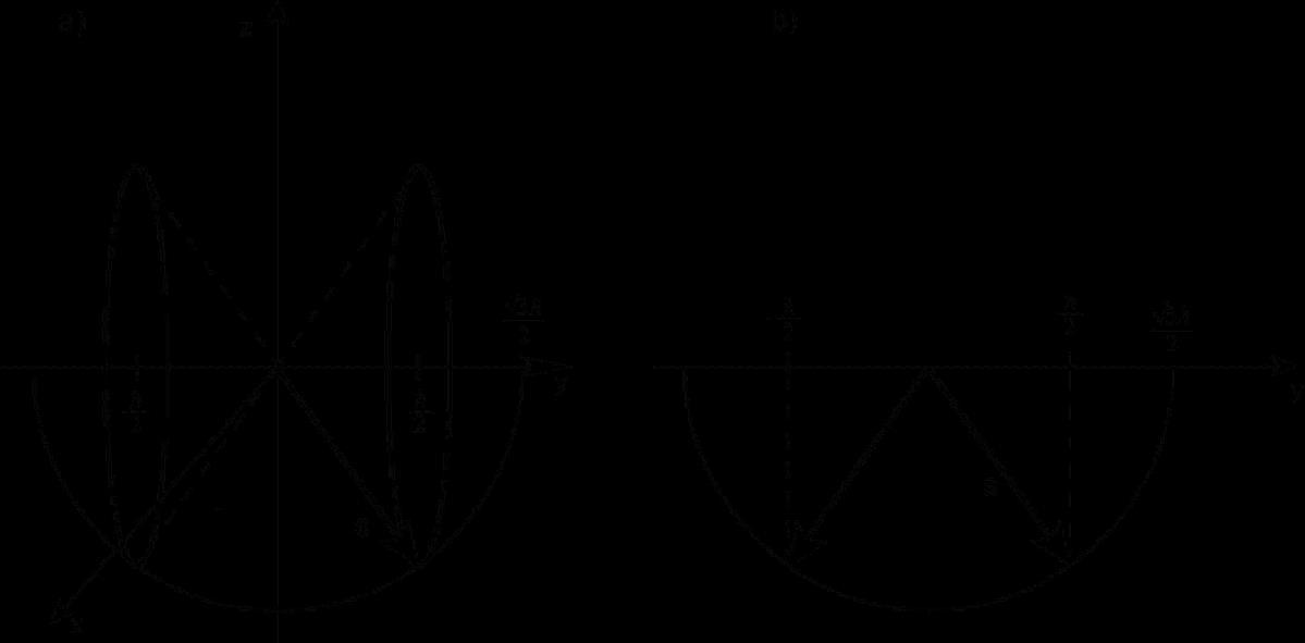
In the vector model, shown below, the spin is precessing around the y-axis at a constant angle such the y-component of the spin is constant and x- and z-components oscillate about zero.
Ch. 2 Solutions 3/20/19 2-10
[S2 ,S x ] 3 2 4 1 0 0 1 2 0 1 1 0 2 0 1 1 0 3 2 4 1 0 0 1 3 3 8 0 1 1 0 0 1 1 0 0 [S2 ,S y ] 3 2 4 1 0 0 1 2 0 i i 0 2 0 i i 0 3 2 4 1 0 0 1 3 3 8 0 i i 0 0 i i 0 0 [S2 ,S z ] 3 2 4 1 0 0 1 2 1 0 0 1 2 1 0 0 1 3 2 4 1 0 0 1 3 3 8 1 0 0 1 1 0 0 1 0
2.11 The commutators in matrix notation are
Ch. 2 Solutions
In abstract notation, the commutators are
x 2S y S y S x
S z 2S y S y S z
S x S x S y S y S x S x
i S z
S y 3 S y 3
S z S z S y S y S z S z S x S y S x
S x S y i S z
S x 0 S z S y S z i S x
S z S y i S x
S x S y S x i S x S z S x S y S x i S z S x S z S y S z i S z S x S z S y S z i S x S z
0 [S2 ,S z ]
S x 2 S y 2 S z 2 ,S z
S y 2S z S z S y 2
S x S x S z S z S x S x
S z 2S z S z S z 2
S y S y S z S z
0 2.12 For S x the diagonalization yields the eigenvalues
i S y S x S y S z S y i S x S y
S z
3/20/19 2-11
[S2 ,S x ] S x 2 S y 2 S z 2 ,S x S x 2 ,S x S y 2 ,S x S z 2 ,S x S x 2S x S x S x 2 S y 2S x S x S y 2 S z 2S x S x S z 2 S x 3 S x 3 S y S y S x S x S y S y S z S z S x S x S z S z 0 S y S x S y i S z S y S x i S z S y S z S x S z i S y S z S x i S y S z S y S x S y i S y S z S y S x S y i S z S y S z S x S z i S z S y S z S x S z i S y S z 0 [S2 ,S y ] S x 2 S y 2 S z 2 ,S y S x 2 ,S y S y 2 ,S y S z 2 ,S y S
2 S y 2S y S y S y 2
2
z
S
S x 2 ,S z
S y 2 ,S
S z 2 ,
z
S x 2S z S z S x 2
S y S y S z 3 S z 3 S x S z S x i S y S x S z i S y S x S y S z S y i S x S y S z i S x S y 0 S x S z S x i S x S y S x S z S x i S y S x S y S z S y
S x 2 0 1 0 1 0 1 0 1 0 2 0 2 2 0 2 0 2 2 2 2 2 0 2 2 0 1 ,0, 1 and the eigenvectors
3/20/19 2-12 2 0 1 0 1 0 1 0 1 0 a b c 1 a b c b a 2 a c b 2 b c 2 a 2 b 2 c 2 1 b 2 1 2 1 1 2 1 b 1 2 ,a 1 2 ,c 1 2 1 x 1 2 1 1 2 0 1 2 1 2 0 1 0 1 0 1 0 1 0 a b c 0 a b c b 0 a c 0 b 0 a 2 b 2 c 2 1 a 2 1 1 1 a 1 2 ,b 0,c 1 2 0 x 1 2 1 1 2 1 2 0 1 0 1 0 1 0 1 0 a b c 1 a b c b a 2 a c b 2 b c 2 a 2 b 2 c 2 1 b 2 1 2 1 1 2 1 b 1 2 ,a 1 2 ,c 1 2 1 x 1 2 1 1 2 0 1 2 1 For S y the diagonalization yields S y 2 0 i 0 i 0 i 0 i 0 i 2 0 i 2 i 2 0 i 2 0 2 2 2 i 2 i 2 0 2 2 0 ,0, and the eigenvectors 2 0 i 0 i 0 i 0 i 0 a b c 1 a b c ib a 2 ia ic b 2 ib c 2 a 2 b 2 c 2 1 b 2 1 2 1 1 2 1 b i 2 ,a 1 2 ,c 1 2 1 y 1 2 1 i 2 0 1 2 1
Ch. 2 Solutions
Ch. 2 Solutions 3/20/19 2-13 2 0 i 0 i 0 i 0 i 0 a b c 0 a b c ib 0 ia ic 0 ib 0 a 2 b 2 c 2 1 a 2 1 1 1 a 1 2 ,b 0,c 1 2 0 y 1 2 1 1 2 1 2 0 i 0 i 0 i 0 i 0 a b c 1 a b c ib a 2 ia ic b 2 ib c 2 a 2 b 2 c 2 1 b 2 1 2 1 1 2 1 b i 2 ,a 1 2 ,c 1 2 1 y 1 2 1 i 2 0 1 2 1 2.13 The commutators are [S x ,S y ] 2 0 1 0 1 0 1 0 1 0 2 0 i 0 i 0 i 0 i 0 2 0 i 0 i 0 i 0 i 0 2 0 1 0 1 0 1 0 1 0 2 2 i 0 i 0 0 0 i 0 i i 0 i 0 0 0 i 0 i 2 2 2i 0 0 0 0 0 0 0 2i i 1 0 0 0 0 0 0 0 1 i S z [S y ,S z ] 2 0 i 0 i 0 i 0 i 0 1 0 0 0 0 0 0 0 1 1 0 0 0 0 0 0 0 1 2 0 i 0 i 0 i 0 i 0 2 2 0 0 0 i 0 i 0 0 0 0 i 0 0 0 0 0 i 0 2 2 0 i 0 i 0 i 0 i 0 i 2 0 1 0 1 0 1 0 1 0 i S x
The eigenvalue equation is
For spin-1 this is
Hence the S2 operator must be 2 2 times the identity matrix:
Ch. 2 Solutions 3/20/19 2-14 [S z ,S x ] 1 0 0 0 0 0 0 0 1 2 0 1 0 1 0 1 0 1 0 2 0 1 0 1 0 1 0 1 0 1 0 0 0 0 0 0 0 1 2 2 0 1 0 0 0 0 0 1 0 0 0 0 1 0 1 0 0 0 2 2 0 1 0 1 0 1 0 1 0 i 2 0 i 0 i 0 i 0 i 0 i S y 2.14 Using the component matrices we find S2 S x 2 S y 2 S z 2 2 0 1 0 1 0 1 0 1 0 2 0 1 0 1 0 1 0 1 0 2 0 i 0 i 0 i 0 i 0 2 0 i 0 i 0 i 0 i 0 1 0 0 0 0 0 0 0 1 1 0 0 0 0 0 0 0 1 2 2 1 0 0 0 2 0 0 0 1 2 2 1 0 0 0 2 0 0 0 1 1 0 0 0 0 0 0 0 1 2 2 1 0 0 0 1 0 0 0 1
S2 sm s s 1 2 sm
S2 1m 2 2 1m
S2 2 2 1 0 0 0 1 0 0 0 1
2.15 a) The possible results of a measurement of the spin component S z are always 1 , 0 , 1 for a spin-1 particle. The probabilities are
The three probabilities add to unity, as they must.
b) The possible results of a measurement of the spin component S x are always 1 , 0 , 1 for a spin-1 particle. The probabilities are
The three probabilities add to unity, as they must.
c) For the first measurement, the expectation value is
For the second measurement, the expectation value is
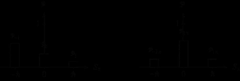
The histograms are shown below.
Ch. 2 Solutions 3/20/19 2-15
P1 1 in 2 1 2 29 1 3i 29 0 4 29 1 2 2 29 11 3i 29 1 0 4 29 1 1 2 2 29 2 4 29 P0 0 in 2 0 2 29 1 3i 29 0 4 29 1 2 2 29 0 1 3i 29 0 0 4 29 0 1 2 3i 29 2 9 29 P 1 1 in 2 1 2 29 1 3i 29 0 4 29 1 2 2 29 11 3i 29 1 0 4 29 1 1 2 4 29 2 16 29
P1x x 1 in 2 1 2 1 1 2 0 1 2 1 2 29 1 3i 29 0 4 29 1 2 1 29 3i 2 29 2 29 2 1 58 2 3i 2 11 58 P0x x 0 in 2 1 2 1 1 2 1 2 29 1 3i 29 0 4 29 1 2 2 2 29 4 2 29 2 36 58 P 1x x 1 in 2 1 2 1 1 2 0 1 2 1 2 29 1 3i 29 0 4 29 1 2 1 29 3i 2 29 2 29 2 1 58 2 3i 2 11 58
S z m P m m 1 4 29 0 9 29 1 16 29 12 29
S x m P mx m 1 11 58 0 36 58 1 11 58 0
2.16 a) The possible results of a measurement of the spin component S z are always 1 , 0 , 1 for a spin-1 particle. The probabilities are
The three probabilities add to unity, as they must.
b) The possible results of a measurement of the spin component S y are always
1 , 0 , 1 for a spin-1 particle. The probabilities are
Ch. 2 Solutions 3/20/19 2-16
P1 1 in 2 1 2 29 1 y 3i 29 0 y 4 29 1 y 2 2 29 11 y 3i 29 1 0 y 4 29 1 1 y 2 2 29 1 2 3i 29 1 2 4 29 1 2 2 1 58 2 3i 2 11 58 P0 0 in 2 0 2 29 1 y 3i 29 0 y 4 29 1 y 2 2 29 0 1 y 3i 29 0 0 y 4 29 0 1 y 2 2 29 i 2 3i 29 0 4 29 i 2 2 1 58 i 2 4 2 36 58 P 1 1 in 2 1 2 29 1 y 3i 29 0 y 4 29 1 y 2 2 29 11 y 3i 29 1 0 y 4 29 1 1 y 2 2 29 1 2 3i 29 1 2 4 29 1 2 2 1 58 2 3i 2 11 58
P1y y 1 in 2 y 1 2 29 1 y 3i 29 0 y 4 29 1 y 2 2 29 y 11 y 3i 29 y 1 0 y 4 29 y 1 1 y 2 2 29 2 4 29 P0y y 0 in 2 y 0 2 29 1 y 3i 29 0 y 4 29 1 y 2 2 29 y 0 1 y 3i 29 y 0 0 y 4 29 y 0 1 y 2 3i 29 2 9 29
The three probabilities add to unity, as they must.
c) For the first measurement, the expectation value is
For the second measurement, the expectation value is
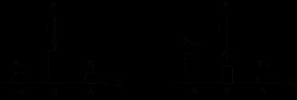
The histograms are shown below.
2.17 a) The possible results of a measurement of the spin component S z are always
1 , 0 , 1 for a spin-1 particle. The probabilities are
The expectation value of S z is
b) The expectation value of S x is
Ch. 2 Solutions 3/20/19 2-17 P 1y y 1 in 2 y 1 2 29 1 y 3i 29 0 y 4 29 1 y 2 2 29 y 11 y 3i 29 y 1 0 y 4 29 y 1 1 y 2 4 29 2 16 29
S z m P m m 1 11 58 0 36 58 1 11 58 0
S y m P my m 1 4 29 0 9 29 1 16 29 12 29
P 1 2 1 0 0 1 30 1 2 5i 2 1 30 1 2 1 30 P0 0 2 0 1 0 1 30 1 2 5i 2 1 30 2 2 4 30 P -1 2 0 0 1 1 30 1 2 5i 2 1 30 5i 2 25 30
S z P P0 0 P 1 30 4 30 0 25 30 24 30 4 5
2.18
a) The possible results of a measurement of the spin component S z are always 1 , 0 , 1 for a spin-1 particle. The
b) After the S z measurement, the system is in the state
measurement of the spin component
c) Schematic of experiment.

Ch. 2 Solutions 3/20/19 2-18 S x S x 1 30 1 2 5i 2 0 1 0 1 0 1 0 1 0 1 30 1 2 5i 1 30 2 1 2 5i 2 1 5i 2 1 30 2 2 2 1 5i 5i 2 2 15
probabilities are P1 1 in 2 1 1 14 1 3 14 0 2i 14 1 2 1 14 11 3 14 1 0 2i 14 1 1 2 1 14 2 1 14 P0 0 in 2 0 1 14 1 3 14 0 2i 14 1 2 1 14 0 1 3 14 0 0 2i 14 0 1 2 3 14 2 9 14 P 1 1 in 2 1 1 14 1 3 14 0 2i 14 1 2 1 14 11 3 14 1 0 2i 14 1 1 2 2i 14 2 4 14
1 . The possible results
a
S x are always 1 , 0 , 1 for a spin-1
The probabilities are P1x x 1 in 2 1 2 1 1 2 0 1 2 1 1 2 1 2 2 1 4 P0x x 0 in 2 1 2 1 1 2 1 1 2 1 2 2 1 2 P 1x x 1 in 2 1 2 1 1 2 0 1 2 1 1 2 1 2 2 1 4
of
particle.
2.19 The probability is
2.20 Spin 1 unknowns. Follow the solution method given in the lab handout. (i) For unknown number 1, the measured probabilities are
3/20/19 2-19
Ch. 2 Solutions
P f f i 2 1 i 7 y 1 2 7 y 0 i 7 y 1 1 6 1 2 6 0 i 3 6 1 2 1 i 7 1 6 y 11 1 i 7 2 6 y 1 0 1 i 7 i 3 6 y 1 1 2 7 1 6 y 0 1 2 7 2 6 y 0 0 2 7 i 3 6 y 0 1 i 7 1 6 y 11 i 7 2 6 y 1 0 i 7 i 3 6 y 1 1 2 1 i 7 1 6 1 2 1 i 7 2 6 i 2 1 i 7 i 3 6 1 2 2 7 1 6 1 2 2 7 2 6 0 2 7 i 3 6 1 2 i 7 1 6 1 2 i 7 2 6 i 2 i 7 i 3 6 1 2 2 1 168 1 i 2 2i 3 i 3 2 2 0 i2 6 i 2 3 2 1 168 5 2 2 2i i 3 i2 6 2 1 168 5 2 2 2 2 3 2 6 2 1 168 64 8 2 4 3 8 6 0 524 or in matrix notation P f f i 2 1 i 7 1 2 i 2 1 2 2 7 1 2 0 1 2 i 7 y 1 2 i 2 1 2 1 6 1 2 i 3 2 1 168 1 2 2 2 2 i 2 1 2 2 1 2 i 3 2 1 168 1 2 2 4 2i i 3 i2 6 2 1 168 64 8 2 4 3 8 6 0.524
P1 1 4 P1x 1 4 P1y 1 P0 1 2 P0x 1 2 P0y 0 P 1 1 4 P 1x 1 4 P 1y 0 Write the unknown state as
Equating the predicted S z probabilities and the experimental results gives
allowing for possible relative phases. So now the unknown state is
Equating the predicted S x probabilities and the experimental results gives
Equating the predicted S y probabilities and the experimental results gives
Ch. 2 Solutions 3/20/19 2-20 1 a 1 b 0 c 1
P1 1 1 2 1 a 1 b 0 c 1 2 a 2 1 4 a 1 2 P0 0 1 2 0 a 1 b 0 c 1 2 b 2 1 2 b 1 2 e i P 1 1 1 2 1 a 1 b 0 c 1 2 c 2 1 4 c 1 4 e i
1 1 2 1 1 2 e i 0 1 2 e i 1
P0 x x 0 1 2 1 2 1 1 1 2 1 1 2 e i 0 1 2 e i 1 2 1 2 2 1 e i 2 1 8 1 e i 1 e i 1 8 1 1 e i e i 1 4 1 cos 1 2 cos 1 Giving the state 1 1 2 1 1 2 e i 0 1 2 1
P1y y 1 1 2 1 2 1 i 2 0 1 2 1 1 2 1 1 2 e i 0 1 2 1 2 1 4 i 2 e i 1 4 2 1 4 1 iei 1 ie i 1 4 1 1 iei ie i 1 2 1 sin 1 sin 1 2 Hence the unknown state is 1 1 2 1 1 2 e i 2 0 1 2 1 1 2 1 i 2 0 1 2 1 1 y
For unknown number 2, the measured probabilities are P1 1 4 P1x 9 16 P1y 0 870 P0 1 2 P0x 3 8 P0y 0 125 P 1 1 4 P 1x 1 16 P 1y 0.005 Write the unknown state as 2 a 1 b 0 c 1
the predicted S z probabilities and the experimental results gives Quantum Mechanics A Paradigms Approach 1st Edition McIntyre Solutions Manual Full Download: http://testbanktip.com/download/quantum-mechanics-a-paradigms-approach-1st-edition-mcintyre-solutions-manual/ Download all pages and all chapters at: TestBankTip.com
(ii)
Equating
