Solutions for Mathematical Applications for The Management Life And Social Sciences 12th Us Edition by 6alsm

Chapter 2: Quadratic and Other Special Functions

Exercises 2.1 __________________________________________________________________

1. 22 2324 2 210 xxx xx  

2. 22 2522 2 3230 xxx xx

3. (1)(2)4 2 324 2 320 yy yy yy

4. (1)(3)1 2 420 zz zz  

5. 2 412 2 4120 2 62120 (6)2(6)0 (6)(2)0 60or20 xx xx xxx xxx xx xx

Solution: x = -2, 6

6. 2 1110xx 2 2 11100 10100 (10)(1)0 100or10 xx xxx xx xx 



Solution: x = 1, 10

7. 2 940 (32)(32)0 320 or 320 x xx xx    Solution: 33 , 22 x 

8. 2 25160 (54)(54)0 540 or 540 x xx xx    Solution: 44 , 55 x 

9. 2 2 0 (1)0 xx xx xx    Solution: x = 0, 1 Never divide by a variable. A root is lost if you divide.

10. 22 43 2 024 02(2) 20 or 20 ttt tt tt tt     Solution: t = 0, –2

11. 2 4410 (21)(21)0 210 tt tt t

   Solution: 1 2 t 

12. 2 491410 (71)(71)0 710 71 zz zz z z

    Solution: 1 7 z 

13.

 2 2 5611 51160 5610 560 or 10 xx xx xx xx     Solution: 6 ,1 5 x 

14.

 2 2 726 7260 71320 7130 or 20 13 ,2 7 xx xx xx xx x     

Chapter 2: Quadratic and Other Special Functions

15. a. 2 440xx a = 1, b = –4, c = –4 2 (4)(4)4(1)(4) 2(1) 432442 222 22 x    

b. Since 21.414,  the solutions are approximately 4.83, –0.83.

c. 2 670xx a = 1, b = –6, c = 7 63628 2 68622 32 22 x     21.414,  the solutions are approximately 4.83, –0.83.

16. 2 670xx a = 1, b = –6, c = 7 63628 2 68622 32 22 x    

a. 32, 32 b. 4.41, 1.59

17. 2 210 ww a = 2, b = 1, c = 1 11817 44 w  

There are no real solutions.

18. 2 240zz

a = 1, b = 2, c = 4 2416212 22 z   No real solutions.

19. 2 42842 22 720 22 1 22 xx x     

a. 122,122  b. 3.83,1.83

20. 2 2 623 3620 6 6 3624 6 122 6 3 66 xx xx x x         a. 3333 , 33  b. 0.42, 1.58

21. 2 7 7 y y  

22. 2 12 12 23 z z z   

23. 2 580 2 16 4 x x x   

24. 2 375 2 25 5 x x x   

25. 2 (4)25 45 45 x x x    Solution: x = 1, –9

26. 2 (1)2 12 12 x x x   

27.  2 521 2 4210 730 xxx xx xx 



 Solution: x = –7, 3

Chapter 2: Quadratic and Other Special Functions

28.  2 17814 2 9140 720 xxx xx xx 

Solution: x =–7, –2

29. 2 40 82 2 4320 (8)(4)0 ww ww ww

80 or 40 ww Solution: w = 8, –4

30. 2 11 10 26 2 31160 (32)(3)0 320 or 30 y y yy yy yy

Solution: 2 , 3 3 y 

31. 2 1616210 zz a = 16, b =16, c = –21 162561344 32 164037 or 3244 z



 Solution: 73 , 44 z 

32. 2 10650 yy

a = 10, b = –1, c = –65 11(2600) 20 126011515052 or 20202020 y

Solution: 513 , 25 y 

33. (1)(5)7 2 457 2 4120 (6)(2)0 xx xx xx xx

 

Solution: x = –6, 2

34. (3)(1)1 2 331 2 440 (2)(2)0 20 xx xxx xx xx x      Solution: x = 2

35. 52622 or 5260xxxx a = 5, b = –2, c = –6 24120131 105 x   Solution: 131131 , 55 x  

36. 2 362 xx 2 3620 xx a = 3, b = 6, c = 2 63624612 66 62333 63 x    

Solution: 3333 , 33 x  

37. 2 217070 xx

Divide by –7 and rearrange. 2 3100 (5)(2)0 xx xx   Solution: x = –2, 5 10 50 100 10

Chapter 2: Quadratic and Other Special Functions

38. 2 31160 xx (3x – 2)(x – 3) = 0 Solution: 2 , 3 3 x  39. 2 30020.010 xx 

a = –0.01, b = –2, c = 300 241224 0.020.02 300 or 100 x

40. 2 9.620.10 xx

2 9.620.10 2 20960 (12)(8)0 xx xx xx

Solution; x = 12, 8 41. 2 25.616.11.10 xx a = 25.6, b = –16.1, c = –1.1 16.1259.21112.64 51.2 16.1371.85 51.2 0.69 or 0.06

Chapter 2: Quadratic and Other Special Functions

42. 2 6.84.92.60 zz

2 6.84.92.60 zz

43. 8 9 2 89 2 980 (8)(1)0 x x xx xx xx     Solution: x = 1, 8

44. 3 1 21 (1)1(2)(1)3(2) 2236 8 x xx xxxxx xx x  

 Solution: x = 8

45. 1 2 11 2 (22)1 2 2310 (21)(1)0 x x xx xxx xx xx    

Solution: 1 2 x  1 is not a root since division by zero is not defined.

46. 53 4 42 5(2)3(4)4(4)(2) 2 2224832 2 46100 2(25)(1)0 zz zzzz zzz zz zz

      2z + 5 = 0 or z – 1 = 0 Solution: 5 , 1 2 z 

 

47.  2 (8)3(8)20 (8)2(8)10 (8)20 or (8)10 xx xx xx

 Solution: x = –10, –9

48.  2 (2)5(2)240 (2)8(2)30

ss ss

 (2)80or(2)30 ss  Solution: s = 10, –1

49. 2 90200 2 120090200 2 0901400 0(20)(70) Pxx xx xx xx 







A profit of $1200 is earned at x = 20 units or x = 70 units of production.

50. 2 160.1100Pxx When P = 180 we have 180160.110022 or 0.116280 0 xxxx   1625611216144 0.20.2 1612 140 or 20 units 0.2 x 

Chapter 2: Quadratic and Other Special Functions

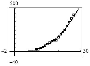
51. a. 2 186400400 2 61,800186400400 Pxx xx

2 18640062,2000 xx

Factoring appears difficult, so let us apply the quadratic formula. 2 640064004(18)(62,200) 36 640036,481,600 36 64006040 10 or 345.56 36 x

So, a profit of $61,800 is earned for 10 units or for 345.56 units.

b. Yes. Maximum profit occurs at vertex as seen using the graphing calculator.

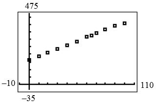
52. a. 2 503000.01 Pxx

When P = 250 we have 2 250503000.01 xx

2 or 0.01505500. xx 50250022 0.02 5049.78 11 or 4989 units 0.02 x 

b. Yes. Try (4000) P and (5000) P . (4000)$250 P  .

53.  2 1009616 2 1001009616 2 09616166 Stt tt

The ball is 100 feet high 6 seconds later.

54. 2 ()1610350 2 01610350 Dttt tt

2 16103500 2 851750 83550 tt tt tt 

The answer 5 t  is the only one that makes sense in this case, so the ball hits the ground at 5 seconds.

55. 2 250.01 ps  a.  2 0250.01 50.150.1 s ss   0 p  if 50.10 s  or 50 s  b. 0 s  . 0 p  means there is no particulate pollution.

56. 2 100 Sxx  a. 0100xx A dosage of 0 or 100 ml gives 0 S  b. Dosage is effective if 0100 x  .

57. 

2 0.0010.73215.417607.738 2 8.990.0010.73215.417607.738 2 89900.73215.417607.738 2 00.73215.4178382.262 txx xx xx xx  

2 15.417(15.417)4(0.732)(8382.262) 2(0.732) 96.996 or 118.058 t tt

  The positive answer is the one that makes sense here, 97.0 mph.

58. 2 0.00460.0336.05Btt  2 2 50.00460.0336.05 0.00460.03311.050 tt tt 

Using the quadratic formula or a graphing utility gives the positive value 45.6. t  The fund is projected to be $5 trillion in the red in the year 2046.

59. 2 0.172.6152.64ptt 2 2 550.172.6152.64 0.172.612.360 tt tt  

Using the quadratic formula or a graphing utility gives the positive value 16.2. t  In 2016 the percent of high school seniors who will have tried marijuana is predicted by the function to reach 55%.

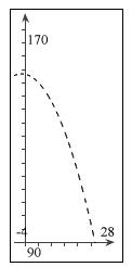
60. a. 2 0.001310yxx  2 0.0013100 9.873 or 779.104 xx xx  

Chapter 2: Quadratic and Other Special Functions

b. 2 4 10 813 x yx 2 4 100 813 115.041or 7.041 x x xx

Given that the distance x is not negative, the first projectile travels further (approximately 779 feet versus the second projectile’s approximately 115 feet). 61. 100 C PC

We know that the selling price is $144 and that the selling price equals the profit plus the cost C to the store. 2 144 100 2 14400100 2 100144000 180 or 80 C C C CC C CC

The cost C of the necklace to the store is not negative, so C= $80 is the amount the store paid for the necklace.

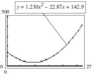
62. 2 1.4825.23416.91yxx  2

Using the quadratic formula or a graphing utility gives the positive value 42. x 

Spending is projected to reach $1968 billion in the year 2032. (1990 + 42 = 2032)

63. 2 4.6143.41620Exx 2 2 70714.6143.41620 4.6143.454510 xx

Using the quadratic formula or a graphing utility gives the positive value 30. x 

The model predicts these expenditures will reach $7071 billion in 2030. (2000 + 30 = 2030)

64.

22 2 20.01 vkRr vr  

In each case below only nonnegative values of r are reported. a.   2 0.0220.01 2 0.010.01 2 0 0 r r r r     b.   2 0.01520.01 2 0.00750.01 2 0.0025 0.05 r r r r    

c.   2 020.01 2 0.01 0.1 r r r   

d In this case the corpuscle is at the wall of the artery.

65. 2 164Kv

In each case below only positive values of K are reported.

a. 2 16(20)4324 18 K K   b. 2 16(60)4964 31 K K  

c. Speed triples, but K changes only by a factor of 1.72.

66. Given that 2 1 16 st  and 2 1090,st  1221 3.93.9 tttt   2 12 1 1 161090 10903.9 42511090 tt t t    2 11 16109042510 tt

Using the quadratic formula or a graphing utility gives the positive value 1 3.70. t 

Chapter 2: Quadratic and Other Special Functions

The depth of the fissure is about 219 ft.

Exercises 2.2

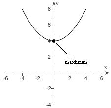
1. 1 2 2 yxx

a. 1 1 22(1/2) b x a

2 11 (1)(1) 22 y

Vertex is at 1 1, . 2 

b. a > 0, so vertex is a minimum.

c. 1

d. 1 2

2. 2 2 yxx 

a. 2 1 22 b x a

When x = 1, y = –1. The vertex is (1, –1).

b. a > 0, so vertex is a minimum.

c. 1

d. 1

3. 2 82 yxx 

a. 2 1 22(1) b x a  2 82(1)(1)9 y 

Vertex is at (1, 9).

b. a < 0, so vertex is a maximum.

c. 1

d. 9

4. 2 642 yxx 

a. 4 1 24 b x a

When x = –1, y = 8. The vertex is (–1, 8).

b. a < 0, so vertex is a maximum.

c. 1

d. 8

5. 2 ()6 fxxx 

a. 6 3. 22 b x a 

 2 36339 f 

Vertex is at  3,9

b. 0, a  so vertex is a maximum.

c. 3

d. 9

6.  2 23fxxx

a.  2 1 221 b x a 

 2 1 12134 f 

Vertex is at  1,4

b. a > 0, so vertex is a minimum.

c. 1

d. 4

7. 2 1 4

yxx 

Vertex is a maximum point since a < 0.

V: 1 2 22(1/4) 1 2 (2)21 4 b x a y 



Zeros: 2 1 0 4 1 10 4 0, 4 xx xx x 

 

y-intercept = 0

Chapter 2: Quadratic and Other Special Functions

2 -2 x y y  x  x 2 1 4

8. 2 218 yxx 

Vertex is a maximum since a < 0.

V: 2 189 242 998116281 218 22222 b x a y

Zeros: 2 0218 02(9) 20 or 90 0 9 xx xx xx xx

y-intercept = 0

10. 2 69yxx

Vertex is a minimum since a > 0.

V: 2 6 3 22 36(3)90 b x a y 

Zeros: 2 069 0(3)(3) 30 3 xx xx x x  

 y-intercept = 9

9. 2 44yxx

Vertex is a minimum point since a > 0.

V: 4 2 22(1) b x a

(2)4(2)40 y

Zeros: 2 44(2)(2)0 2 xxxx x

y-intercept = 4

Zeros: 22 1 30260 2 2424227 17 22 xxxx x    -intercept =3 y -5510 x 25 50 y y =–2 x 2 + 18 x 2 44yxx -4-2 4 x y 246 x -5 5 10 y y = x 2 – 6x + 9

11. 2 1 3 2 yxx

Vertex is a minimum point since a > 0.

V: 2 1 1 22(1/2) 17 (1)(1)3 22 b x a y 

Vertex

Chapter 2: Quadratic and Other Special Functions

13. 2 (3)1yx

a. Graph is shifted 3 units to the right and 1 unit up.

14. 2 (10)1yx

a. Graph is shifted 10 units to the right and 1 units up.

Zeros: Using the quadratic formula,

15. 2 (2)2yx a. Graph is shifted 2 units to the left and 2 units down. b.

Chapter 2: Quadratic and Other Special Functions

16.  2 128 yx

a. Graph is shifted 12 units to the left and 8 units down.

17. 2 115 22yxx

V: 2 (1) 1 22(1/2) 115(1)18 22 b x a y 

Zeros: 2 215(5)(3)0 5, 3 xxxx x  

18.

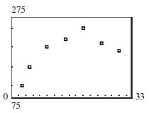
From the graph, the vertex is approximately   2,3.5 . The zeros are approximately –8 and 4. Algebraic check:

V: x-coordinate: 4 2 22 b a  y-coordinate: 0.1(4 – 8 – 32) = –3.6

So, actual vertex is (–2, –3.6)

Zeros: 2 0432(8)(4) 8, 4 xxxx x  

19. 2 1 312 4 yxx

V: 2 3 6 1 2 2 4 1 (6)3(6)123 4 b x a y 

Zeros: 2 2 12480 41441920 xx bac  

There are no zeros.

20. 2 25yxx

2 25yxx

From the graph, the vertex is (1, 4).

There are no real zeros.

Algebraic check:

V: x-coordinate: 2 1 22 b a  y-coordinate: 2 12(1)54 

The discriminant is negative, so no real zeros.

21. 2 ()5 fxyxx  Average Rate of Change (1)(1) 1(1) 6410 5 22 ff

22. 2 ()830.5 fxyxx 

Average Rate of Change (4)(2) 42 281612 6 22 ff

Chapter 2: Quadratic and Other Special Functions

23. 2 630.20.01 yxx 

V: 0.2 10 0.02 632164 x y  

Zeros: 2 206300(90)(70)0 90, 70 xxxx x 

24. 2 0.216140yxx

V: x-coordinate: 16 40 22(0.2) b a 

y-coordinate: 2 0.2(40)16(40)140180 

Zeros: 2 00.2(80700) 0.2(70)(10) 70, 10 xx xx x 

Graphing range: x-min = –100 y-min = –200 x-max = 0 y-max = 50

25. 2 0.00010.01yx

V: 0 0 2(0.0001) 00.010.01 x y  

Zeros: 22 0.00010.010.010.0110

0.01(0.11)(0.11)0 10, 10 xx xx x 

26. 2 0.010.0010.001(10) yxxxx 

Zeros: x = 0, x = 10

V: x-coordinate: 0.01 5 20.002 b a  y-coordinate: 0.01(5) – 0.001(25) = 0.025

Graphing range: x-min = –5 y-min = –0.1 x-max = 15 y-max = 0.1

27. 2 ()81616 fxxx a. 16 1 216 b x a

and

124

b. Graphical approximation gives 0.73,2.73 x 

28. 2 ()31816 fxxx a. 18 3 26 b x a  and

2 31816yxx

b. Graphical approximation gives 1.085,4.915 x 

Chapter 2: Quadratic and Other Special Functions

29. 2 ()384 fxxx

a. The TRACE gives 2 x  as a solution.

b.   2 x is a factor.

c.  2 384232 xxxx 

d. 2320 20 or 320 xx xx   Solution is 2,2/3 x 

30. 2 ()527 fxxx

a. The TRACE gives 1 x  as a solution.

b.  1 x  is the factor.

c.  2 527157 xxxx 

d. 1570 10or 570 xx xx 

Solution is 1,7/5 x 

31. 2 160.01900Pxx

The vertex coordinates are the answers to the questions.

a. a = –0.01, b = 16 16 800 20.02 b x a 

Profit is maximized at a production level of 800 units.

b.  2 (800)168000.01(800)900$5500

is the maximum profit.

32. 2 800.0412,000Pxx

The vertex coordinates are the answers to the questions.

a. a = –0.04, b = 80 80 1000 20.08 b x a 

Profit is maximized at a production level of 1000 units.

b.  2 (1000)8010000.04100012,000 $28,000 is the maximum profit.

33. 2 800 Yxx 

Opens down so maximum Y is at vertex.

V: 800 400 2 x 

Maximum yield occurs at x = 400 trees.

34. 2 ykx 

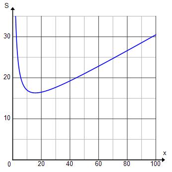
35. 2 1000 Sxx 

Maximum sensitivity occurs at vertex.

V: 1000 500 2 x 

The dosage for maximum sensitivity is 500.

x S

36. 2 50 Axx  x-coordinate of the vertex = 50 25 22 b a 

A length of 25 feet and width of 25 feet gives a maximum area of 625 square feet. 12345 5 10 15

Chapter 2: Quadratic and Other Special Functions

37. 2 27090 Rxx  Maximum rate occurs at vertex. V: 2703 2(90)2 x  (lumens) is the intensity for maximum rate.

40. 2 2 2 1960(10) 10 1960 1 10 1960 vh vh hv   

38. 2 11216 stt  t-coordinate of the vertex = 112 3.5 seconds 232 b a

At t = 3.5, 2 112(3.5)16(3.5)196 feet s 

39. a. 2 0.001310yxx V: 1 384.62; 0.0026 x  2 0.0013(384.62)384.6210 202.31 y

b. 2 14 10 813 yxx

V: 4 3 54 2 81 x  ; 2 14 813(54)(54)1046 y 

Projectile a. goes 202.31 – 46 = 156.31 feet higher.

41. a. From b to c. The average rate of change is the same as the slope of the segment. The segment from b to c is steeper.

b. Needs to satisfy db  to make the segment from a to d have a greater slope.

42. a. From b to c. The average rate of change is the same as the slope of the segment. The segment from b to c has a negative slope.

b. Needs to satisfy db  to make the segment from a to d have a greater slope.

43. a. No. of AptsRentTotal Revenue

50$1800$90,000

49$1860$91,140

48$1920$92,160

b. Revenue increases $2,160

c.     50180060 Rxx  d. 2 60120090,000Rxx  R is maximized at  1200 10 260 x  Rent would be   $1800$6010$2400. 

44. a. PriceNo. of skatersTotal Revenue 1250$600 1160$660 1070$700

b. The revenue increases.

c. ()120.5505 Rxxx  where x is the number of each additional 5 skaters.

Chapter 2: Quadratic and Other Special Functions

d. 2 ()2.535600 Rxxx . Maximum revenue is at 35 7 5 x  , or 85 skaters.

45. a. A quadratic function or parabola.

b. 0 a  because the graph opens downward.

c. The vertex occurs after 2004 (or when 0 x  ), so 0. 2 b a  Hence with 0 a  we must have 0. b  The value (0) cf  or the yvalue during 2004 which is positive.

46. 2 yaxbxc 

Zeros: (0, 0) and (40, 0)

Vertex: , 40 2 b a    (0, 0): 2 2 0(0)(0) 0 So, abc c yaxbx    (40, 0): 0160040 40 2 So, 40 ab ba yaxax   

So, x-coordinate of the vertex = 40 20 2 a a 

When x = 20, y = 40 2 40(20)40()(20) 40400800 40040 aa aa a    1 and 4 10 ab

The equation is 1 2 4 10 yxx 

47. 2 20.61116.47406yxx 

For 2010, 10 x  gives 8303. y  For 2015, 15 x  gives 10,297.25. y  For 2020, 20 x  gives 13,322. y 

Average rate of change from 2010 to 2015:

10,297.258303 398.85 1510 

Average rate of change from 2015 to 2020: 13,32210,297.25 604.95 2015 

To the nearest dollar, the projected average rate of change of U.S. per capita health care costs from 2010 to 2015 will be $399/year, and from 2015 to 2020 it will be $605/year.

48. a.

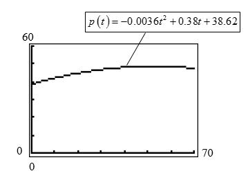
b. Using the equation, we identify the maximum point by computing

0.38 52.78 220.0036 52.7848.65 b t a p  

The maximum point is (52.78, 48.65).

c. According to this model, the maximum percentage of women in the workforce occurs in the year 1970532023. 

49.

50. The graphing calculator gives a minimum point at   9.3,36.6.

Chapter 2: Quadratic and Other Special Functions

Exercises 2.3 __________________________________________________________________

1. 2 ()402000Cxxx

130 Rxx 

2 402000130 2 9020000 (40)(50)0 xxx xx xx

x = 40 or x = 50

Break-even values are at x = 40 and 50 units.

2. At the break-even point, R(x) = C(x). 3600251751122 22 2 15036000 (120)(30)0 xxxx xx xx

x = 120 or x = 30 units

3. 2 ()15,000350.1 Cxxx  2 ()3850.9 Rxxx

15,000350.13850.922 2 35015,0000 (300)(50)0 xxxx xx xx

x = 300 or x = 50

4. At the break-even points, R(x) = C(x). 2 160016001500 2 01001600 0(20)(80) xxx xx xx 

x = 20 or x = 80 units

5. 2 ()11.50.1150 Pxxx





At the break-even points, P(x) = 0. 2 011.50.1150 2 0.111.51500 (15)(100)0

 xx xx xx

Since production < 75 units, x = 15.

6. 2 ()1100120 Pxxx 

At the break-even points, P(x) = 0. 2 01100120 2 12011000 (110)(10)0 xx xx xx   

Since production < 100 units, x = 10.

7. 2 ()3960.9 Rxxx 

a = –0.9, b = 396

Maximum revenue is at the vertex.

V: 396 220 total units 1.8 x  2 (220)396(220)0.9(220)$43,560R 

8. 2 ()1600 Rxxx 

Maximum occurs at the vertex. x-coordinate = 1600 800 2  2 (800)1600(800)(800)$640,000R 

9. 2 ()(1750.50)1750.5 Rxxxxx 

a = –0.50, b = 175

Revenue is a maximum at 175 175. 1 x 

Price that will maximize revenue is p = 175 – 87.50 = $87.50.

10. D: 16001600 pxxp 

Revenue: (1600) 2 1600 Rpxpp Rpp  

Max. revenue for 1600 $800 2 p 

11. 2 ()1101000 Pxxx

Maximum profit is at the vertex or when 110 55. 2 x    55$2025. P 

Chapter 2: Quadratic and Other Special Functions

12. 2 ()881200Pxxx

The x-coordinate giving the maximum profit is 88 44. 22 b a  2 (44)88(44)(44)1200$736P 

13. a.

b.   400,9000 is the maximum

c. positive

d. negative

e. closer to 0

14. a.

b.   125,1125 is the maximum

c. positive

d. negative

e. closer to 0

15. 2 ()3850.9 Rxxx  2 ()15,000350.1 Cxxx 

a. 22 ()3850.9(15,000350.1) 2 35015,000 Pxxxxx xx  

At the vertex we have 350 175. 2 x  So, P(175) = $15,625.

b. No. More units are required to maximize revenue.

c. The break-even values and zeros of P(x) are the same.

16. a. ()()() 2 1600(16001500) 2 1001600 PxRxCx xxx xx   

x-coordinate of max is 100 50 2  2 (50)100(50)(50)1600$900P 

b. No. More units are required to maximize revenue.

c. 2 01001600 2 10016000 (80)(20)0 xx xx xx   

The x-coordinates are the same.

17. a. 2 ()28,000222 5 Cxxx    2 2 22228,000 5 xx  33 2 ()1250125055 Rxxxxx

(The key is “per unit x.”) ()() 3222 125022228,000 55 2 102828,0000 (1000)(28)0 RxCx xxxx xx xx 

Break-even values are at x = 28 and x = 1000.

b. Maximum revenue occurs at 1250 1042 (rounded). 6 5 x  1042$651,041.60 R  is the maximum revenue.

c. 3222 ()125022228,000 55 2 102828,000 Pxxxxx xx

Maximum profit is at 1028 514. 2 x 

  514$236,196 P  is the maximum profit.

d. Price that will maximize profit is 3 1250(514)$941.60. 5 p 

Chapter 2: Quadratic and Other Special Functions

d. The model fits the data quite well.

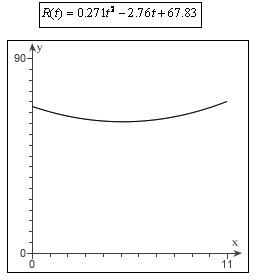
20. 2 ()0.0310.7760.179 Rttt 

a. Maximum occurs at the vertex. The tcoordinate of the vertex is 0.776 12.5. 0.062  Maximum revenue occurred during 2019. The maximum revenue predicted by the model is (12.5)$5.035 million. R 

b. The entry in the table for 2019 is $5.0913 million, so the values are close.

d. 1 Selling price1500 4 x  . When x = 20, 1 1500(20)$1495 4 p

19. a. 5.1 t  , in 2015; $60.79billion R 

b. The data show a smaller revenue, R = $60.27 billion in 2015.

0 0 7 15 2 ()0.0310.7760.179 Rttt 

d. Although there are differences, the model appears to be a good quadratic fit for the data.

21. a.   2 2 2 0.0310.7760.179 0.0120.4920.725 0.0190.2840.546 ptRtCt tt tt tt

b.  0.284 20. ; . 019 75  maximum profit occurred during 2014 (or perhaps in 2015)

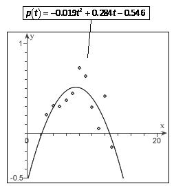
d. The model projects decreasing profits, and, except for 2019, the data support this.

Chapter 2: Quadratic and Other Special Functions

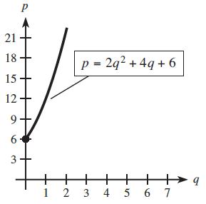
22. a. Supply: 2 816pqq (see below)

24. a. Supply: 2 822pqq (see below)

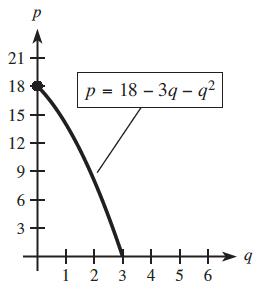
Demand: 2 1 1984 4 pqq  (see below)

Demand: 2162 pq  (see below)

b. See E on the graph.

c. Supply = Demand 2 8162162 2 102000 (10)(20)0 qqq qq qq

 q = 10 (only positive value) p = 216 – 2(10) = 196 q = 10, p = $196

23. a. Supply: 1 2 10 4 pq (see below)

Demand: 2 8663 pqq  (see below)

b. See E on graph.



c. 1 22 108663 4 22 403442412 2 01324304 0(4)(1376) qqq qqq qq qq

 

 q = 4 must be positive. 1 2 (4)1014 4 p  E: (4, 14)

b. See E on the graph.

c. Supply = Demand 1 22 8221984 4 2 5487040 (588)(8)0 qqqq qq qq



  q = 8 (only positive value)

When q = 8, 2 (8)8(8)22 150 p p   So, E = (8, 150).

25. 2 816pqq 2 36436pqq 2281636436

2 424200 2 22100 (221)(10)0 10 qqqq qq qq qq q





   2 108(10)16196 p  E: (10, 196)

26. S: 2 820pqq D: 2 1004 qqp 22 8201004 2 212800 2(10)(4)0 qqqq qq qq



  q = 4 (only positive value) When q = 4, 2 48(4)20$68 p  Equilibrium point: (4, 68)

Chapter 2: Quadratic and Other Special Functions

27. 2 41600pq 2 30020 pq  (3002)41600 61300 2 216 3 qq q q 

 1300 22 41600 or 6 733.33 or 27.08 pp p

E: 2 216, 27.08 3

28. S: 4p – q = 42 or q = 4p – 42 D: 2100 (2)2100 or 2 pqq p   2100 442 2 2 434842100 2 43421840 2(239)(28)0 p p pp pp pp

p = 28 (only positive value) When p = $28, q = 4(28) – 42 = 70

Equilibrium point: (70, 28)

29. 10 or 10 pqqp  2102100 2100 210 2100 10 210 qp q p p p

102102100 2 2301002100 2 23020000 2 1510000 40250 pp pp pp pp pp

40 or 25 pp

(only the positive answer makes sense here) 401030 q  :30,40 E

30. S: 2p – q + 6 = 0 or q = 2p + 6

D: (p + q)(q + 10) = 3696

Substitute 2p + 6 for q in D and solve for p (36)(216)3696 2 66036000





2 106000 (30)(20)0 pp pp pp pp



p = 20 (only positive value)

When p = 20, q = 2(20) + 6 = 46. Equilibrium point: (46, 20)

31. 2p – q – 10 = 0 (p + 10)(q + 30) = 7200 So, (10)(21030)7200 2 201003600





2 2035000 (70)(50)0 50 pp pp pp pp p

  

q = 2(50) – 10 = 90

E: (q, p) = (90, 50)

32. S: 50 250 or 2 q pqp  

D: 10020 10020 or q pqqp q   5010020 2 2 5020040 2 102000 (20)(10)0 qq q qqq qq qq

 





q = 10 (only positive value)

When q = 10, p = 30

Equilibrium point: (10, 30)

33. 11 52227 22 pqq 



 



So, 1 2710(30)7200 2 (74)(30)14,400 2 10412,1800 (174)(70)0 qq qq qq qq

  1 (70)2762 2 p 

E: (70, 62)

Exercises 2.4

Chapter 2: Quadratic and Other Special Functions

q = 5 (only positive value) When q = 5, Equilibrium point: (5, 40)

Chapter 2: Quadratic and Other Special Functions

5 5 5 x y 5 3 2;1 1;1 xx y xx

5 5 5 x y

5 2 ;2 4;2 xx y xx   

5 5 5 x y



5 2

29. 2 1 () x Fx x 

a. 1 1 18 9 1 33 3 F

b. 100199 (10) 1010 F  2 1 () x Fx x 

c. 1 1 18 9 1 33 3 F

d. 100199 (10) 1010 F 

e. 0.00000110.999999 (0.001) 0.0010.001 999.999 F  

f. (0) F is not defined–division by zero.

30. ()1Hxx

a. H(–1) = 2

b. H(1) = 0

c. H(0) = 1

d. No

31. 3/2 () fxx 

a. 3 (16)(16)64 f 

b. 3 (1)(1)1 f 

c. 3 (100)(100)1000 f 

d. 3 (0.09)(0.09)0.027 f 

32. 42 if 0 () 4 if 04 xx kx xx 

a. 0.1420.14.2 k 

b. 0.10.143.93.9 k 

c. 3.93.940.10.1 k 

d.  4.1 k is undefined

33. 2if 0 ()4if 01 1if 1 x kxxx xx  

a.   5 k = 2 since x < 0.

b. 0044 k 

c. 1110 k 

c. 70 g  d. 3.943.90.1 g  1 x y x 

d. 0.0012 k  since x < 0.

34. 0.54if 0 ()4if 04 0if 4 xx gxxx x 

a. 40.544242 g 

b.   1413 g 

Chapter 2: Quadratic and Other Special Functions

35. 1.60.124 yxx  a.

b. polynomial

c. no asymptotes

d. turning points at x = 0 and approximately x = –2.8 and x = 2.8

36. 43 4 () 3 fxxx 

b. polynomial

c. no asymptotes

d. turning point at x = 3 37. 24 1 x y x

38. 3 () 2 fxx x  

b. rational

c. vertical: x = –2 horizontal: x = 1

d. no turning points 39. if 0 () 5 if 0 xx fx

b. piecewise

c. no asymptotes

d. turning point at x = 0.

b. rational

c. vertical: x = –1 horizontal: y = 2

d. no turning points

Chapter 2: Quadratic and Other Special Functions

40. 21if 1 () if 1 xx fx xx

b. piecewise

c. no asymptotes

d. no turning point (there is a jump at x = 1).

41. 2 ()(1084) VVxxx 

a. V(10) = 100(68) = 6800 cubic inches V(20) = 400(28) = 11,200 cubic inches

b. 10840

44. 1.54 0.11 CW 

a. 1.54 W is “close” to 2 W . The graph is turning up. b.

43. 0.30 200.8 yx  a. downward

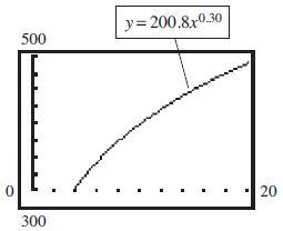
c. Intersecting the graphs of 0.30 200.8 yx  and 443.202416 y  gives 14. x  The number of Internet users in Latin America is expected to reach 443,202,416 (about 443 million) in 2010 + 14 = 2024.

Chapter 2: Quadratic and Other Special Functions

45. 7300 () 100 Cpp p 

a. 0100 p 

b. 730045 (45)$5972.73 10045 C 

c. 730090 (90)$65,700 10090 C 

d. 730099 (99)$722,700 10099 C 

e. 7300(99.6) (99.6)$1,817,700 10099.6 C 

f. To remove p% of the pollution would cost C(p). Note how cost increases as p (the percent of pollution removed) increases.

46. 50,000105 Cx x  

a.  50,0001053000 3000$121.67 3000 C  

x C 100020003000

c. Yes. 50,000 ()105Cx x 

47. A = A(x) = x(50 – x)

a. (2)24896A  square feet (30)3020600A  square feet

b. 0 < x < 50 in order to have a rectangle.

48. 58if 020 () 580.4(20)if 20 x fx xx      

a. 0.3$58 f 

b.  30580.43020$62 f 

c.  40580.44020$66 f 

d. (see graph at right)

Chapter 2: Quadratic and Other Special Functions

49. 2 2 5.5993.5633for 055 6.5651920,900for 5590 xxx y xxx  

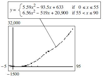
b.  2 505.595093.550633$9933 y  billion ($9.933 trillion)

c.  2 756.56755197520,900$18,875 y  billion ($18.875 trillion)

50. a. C(5) = 7.52 + 0.1079(5) = $8.06

b. C(6) = 19.22 + 0.1079(6) = $19.87

c.  3000131.3450.03213000$227.65 C 

51. a. 49 if 01 70 if 12 () 91 if 23 112 if 34 x x Px x x  

b.   1.270; P  it costs 70 cents to mail a 1.2-oz letter.

c. Domain: 04; x  Range:   49,70,91,112

d. The postage for a 2-ounce letter is 70 cents; for a 201-ounce letter, it is 91 cents.

52. a. 0.10 if 018,550 ()0.15(18,550)1,855 if 18,55075,300 0.25(75,300)10,367.50 if 75,300151,900

b.  

70,0000.1570,00018,5501,855$9,572.50 T 

c.  

 100,0000.25100,00075,30010,367.50$16,542.50 T 

75,3000.1575,30018,5501,855$10,367.50 T

75,3010.2575,30175,30010,367.50$10,367.75 T 

Jack’s tax went up $0.25 for the extra dollar earned. He is only charged 25% on the money he earns above $75,300.

Chapter 2: Quadratic and Other Special Functions

b. A turning point indicates a minimum or maximum cost.

c. This is the fixed cost of production.

Exercises 2.5

1. Linear: The points are in a straight line.

2. Power

3. Quadratic: The points appear to fit a parabola.

4. Linear

5. Quartic: The graph crosses the x-axis four times. Also there are three bends.

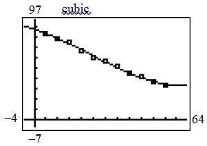
6. Cubic

7. Quadratic: There is one bend. A parabola is the best fit.

8. Cubic 9. y = 2x – 3 is the best fit.

y = 1.5x – 4 is the best fit.

Chapter 2: Quadratic and Other Special Functions

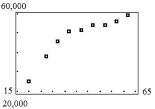
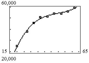
21. a.

b. quadratic

c. 2 251yxx

22. a.

b. quadratic

c. 2 331 xx

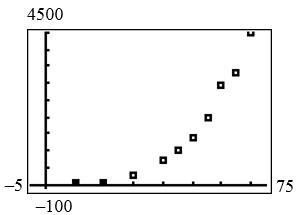
23. a.

b. cubic

c. 3 51yxx

24. a.

b. cubic

c. 32 23 yxxx 

25. a. 154.035,860yx

b.  27154.02735,86040,018 y 

The projected population of females under age 18 in 2037 is 40,018,000.

c. 45,000154.03586059.35 xx 

This population will reach 45,000,000 in 2010 + 60 = 2070 according to this model.

26. a. 18.96321.5yx

b.  1418.9614321.5586.9 y  million metric tons

c. 18.96; m  each year since 2010, carbon dioxide emissions in the U.S. are expected to change by 18.96 million metric tons.

27. a. A linear function is best; 327.69591yx

b.  17327.6179591$15,160 y  billion

c. 327.6 m  means the U.S. disposable income is increasing at the rate of about $327.6 billion per year.

28. a. 0.46512.0yx

b.  180.4651812.020.4% y 

c. 250.46512.028 xx 

This model predicts that the percent of U.S. adults with diabetes will each 25% in 2000 + 28 = 2028.

29. a. 2 0.00520.6215yxx 

b.  0.62 59.6 220.0052 b x a 

c. No, it is unreasonable to feel warmer for winds greater than 60 mph.

30. a. 2 0.04722.6412.1yxx 

b. A maximum occurs at approximately  28.0,48.9. The model predicts that in the year 2000 + 28 = 2028, developing economies reach their maximum share, 48.9%, of the GDP.

31. a.

b. 2 106287028,500yxx 

c. 32 1.7072.919705270yxxx 

Chapter 2: Quadratic and Other Special Functions

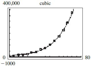
The cubic model fits better.

32. a. 2 0.003360.01274.47yxx 

b. 32 0.00005370.007380.06094.63yxxx 

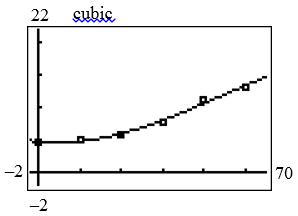
d. The fits look to be equally close.

33. a. 0.01572.01yx

b. 2 0.001050.3671.94yxx 

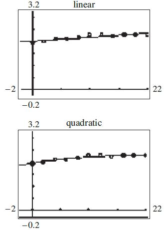
d. The quadratic model is a slightly better fit.

34. a. 1.0388.1yx b. 32 0.0002520.01780.075687.8yxxx 

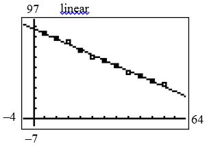
d. The cubic model indicates that the percent of energy use may increase after 2035.

35. a.

Chapter 2: Quadratic and Other Special Functions

A cubic model looks best because of the two bends.

b. 32 0.864128661062,600yxxx 

d. Using the coefficient values reported by the calculator, the model estimates the median income to be $56,250 at age 57.

36. a.

It appears that both quadratic and power functions would make good models for these data.

b. power: 2.74 0.0315 yx  quadratic: 2 1.7671.0679yxx 

c. power: 70$3661 y  billion quadratic: 70$4335 y  billion

The quadratic model more accurately approximates the data point for 2020.

d. 75$5257 y  billion; $5257 billion is the national health-care expenditure predicted by the model for 2025.

37. a. 2.73 0.0514 yx  b.

c. 30$546 y  billion

Chapter 2: Quadratic and Other Special Functions

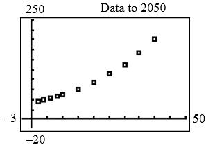
b. Possible models are linear: 2.532162.2yx quadratic: 2 0.0010202.633160.7yxx  cubic: 32 0.000074560.010302.191163.5yxxx 

c. linear: 90390.08 y  quadratic:   90389.36 y  cubic:   90389.77 y 

The linear model most accurately approximates the data point for the year 2040.

d. Replacing y with 425 in the linear model gives 103.8. x  The U.S. population is predicted to reach 425 million in 1950 + 104 = 2054.

Chapter 2: Quadratic and Other Special Functions

Chapter 2 Review Exercises

1. 2 2 3105 350 (35)0 xxx xx xx 

 5 0 or 3 xx

2. 2 430 (43)0 xx xx   4 0 or 3 xx

3. 2 560 (3)(2)0 xx xx   x = –3 or x = –2

4. 2 111020 xx  a = –2, b = –10, c = 11 1010088547 42 x  

5. 2 2 (1)(3)8 238 250 xx xx xx 

2 40bac No real solution

6. 2 2 43 3 4 33 42 x x x  

7. 22 2 2032015 353200 (75)(54)0 xxx xx xx    54 or 75 xx

8. 22 2 8818 16810 xxx xx   a = 16, b = 8, c = –1 8646412 324 x  

9. 2 72.070.02xx 2 0.022.0770 xx a = 0.02, b = –2.07, c = 7 2.074.28490.562.071.93 0.040.04

100 or 3.5 x   

10. 2 46.31170.50 xx a = –0.5, b = 46.3, c = –117 46.32143.69(234) 46.343.7 11

90 or 2.6 x    

11. 2 4250 z 

22 450 z  The sum of 2 squares cannot be factored. There are no real solutions.

12. 2 ()627 fzzz

From the graph, the zeros are –9 and 3. Algebraic solution: 2 (6)27 6270 (9)(3)0 zz zz zz    z = –9 or z = 3 5 25 75 5

Chapter 2: Quadratic and Other Special Functions

2 318480 xx

2 3(616)0 3(8)(2)0 xx xx

x = –2, x = 8

14. 2 ()369 fxxx

2 3690 3230 3310 xx xx xx

15. 2 0 xaxb

To apply the quadratic formula we have “a” = 1, “b” = a, and “c” = b. 2 4 2 aab x 

16. 2240xrarxc

To solve for r, use the quadratic formula with “ a” = x, “b” = –4a, and “c ” 2 xc  22 23 2323 4164() 4164 22 42424 2 aaxxcaaxc r xx aaxcaaxc xx 

17. 2 0.00214.123.10 xx  14.1198.810.184814.114.107 0.0040.004 7051.64, 1.64,or1.75 (using 14.107) x   

18. 2 1.032.021.0150 xx a = 1.03, b = 2.02, c = –1.015 2.024.08044.18182.022.87 2.062.06 2.38 or 0.41 x 

20. 2 1 4 4 yx 

Chapter 2: Quadratic and Other Special Functions

V: x-coordinate = 0

y-coordinate = 4 (0, 4) is a maximum point

y-intercept:  2 1 404 4 

Zeros are 4. x 

21. 2 6 yxx 

a < 0, thus vertex is a maximum.

V: 2 11 2(1)2 1125 6 224 x y 

y-intercept: 2 6006 

Zeros: 2 60 (3)(2)0 xx xx   x = –2, 3

22. 2 45yxx

V: x-coordinate 4 2 2 

y-coordinate 2 24(2)51

(2, 1) is a minimum point.

y-intercept:  2 04055 

Zeros: Since the minimum point is above the xaxis, there are no zeros.

23. 2 69yxx a > 0, thus vertex is a minimum.

V: 2 6 3 2(1) (3)6(3)90 x y  

y-intercept:   2 06099 

Zeros: 2 690 (3)(3)0 3 xx xx x   

-424 2 4 6 x y maximum 246 2 4 6 x y minimum -6-4-22 2 8 x y minimum

24. 2 1294 yxx 

V: x-coordinate 123 82  y-coordinate 2 33 12940 22 

Chapter 2: Quadratic and Other Special Functions

3 , 0 2    is a maximum point.

y-intercept:  2 1209409 

Zeros: From the vertex we have that 3 2 x  is the only zero.

25. 2 1 3 3 yx

V: (0, –3)

Zeros: 2 2 1 30 3 9 3 x x x   

26. 2 1 2 2 yx

Vertex: (0, 2)  minimum No zeros.

The graph using x-min = –4 y-min = 0 x-max = 4 y-max = 6 is shown below.

27. 2 25yxx

V: (–1, 4)

There are no real zeros.

28. 2 107 yxx 

Vertex: 79 , maximum 24

Zeros: 2 7100 (5)(2)0 xx xx

x = 5 or x = 2

Graph using x-min = 0 y-min = –5 x-max = 8 y-max = 5

29. 2 200.1 yxx 

Zeros: x(20 – 0.1x) = 0 x = 0, 200

(This is an alternative method of getting the vertex.)

The x-coordinate of the vertex is halfway between the zeros.

V: (100, 1000)

Chapter 2: Quadratic and Other Special Functions

30. 2 501.50.01 yxx 

Vertex: (75, –6.25)  minimum

37. a. 2 () fxx 

Zeros: 2 2 0.011.5500

0.01(1505000)0

0.01(50)(100)0 xx xx xx

x = 50 or x =100

Graph using x-min = 0 y-min = –10 x-max = 125 y-max = 10

b. 1 ()fx x 

31. (50)(30)25002100400 20 50302020 ff 

32. (50)(10)10221781200 30 50104040 ff

33. a. The vertex is halfway between the zeros. So, the vertex is 1 1, 4. 2 

b. The zeros are where the graph crosses the x-axis. x = –2, 4.

c. The graph matches B.

34. From the graph,

a. Vertex is (0, 49)

b. Zeros are 7. x 

c. Matches with D.

35. a. The vertex is halfway between the zeros. So, the vertex is (7, 24.5).

b. Zeros are x = 0, 14.

c. The graph matches A.

36. From the graph,

a. Vertex is (–1, 9).

b. Zeros are x = –4 and x = 2.

c. Matches with C.

c. 1/4 () fxx  38. 2 if 0 () 1 if 0 xx fx x x  

2 (0)(0)0 f

1 (0.0001)10,000 0.0001 f

c. 2 (5)(5)25

1 (10)0.1 10 f

39. if 1 () 32if 1 xx fx xx

c. (1)1 f 

Chapter 2: Quadratic and Other Special Functions

d. (2)3224 f 

40. if 1 () 32if 1 xx fx xx

41. a. 2 ()(2)fxx

b. ()(1)3fxx

42. 3239 yxxx 

Using x-min = –10, x-max = 10, y-min = –10, y-max = 35, the turning points are at x = –3 and 1.

43. 3 9 yxx 

Using x-min = –4.7, x-max = 4.7, y-min = –15, y-max = 15, the turning points are at x = 1.732.

Note: Your turning points in 42–43. may vary depending on your scale. 44. 1 2 y x 

There is a vertical asymptote x = 2. There is a horizontal asymptote y = 0.

Vertical asymptote is x = –3. Horizontal asymptote is y = 2.

46. a.

b. y = –2.1786x + 159.8571 is a good fit to the data.

Chapter 2: Quadratic and Other Special Functions

c. 2 0.08180.2143153.3095 yxx is a slightly better fit.

47. a.

b. 3.13140yx is a good fit to the data.

c. The quadratic function 2 0.47918.658.4yxx  is a better fit.

48. 2 963216 Stt 

a. 2 16(62)0 tt  2424 2 1.65 or 3.65 t tt

b. 0 t  Use t = 3.65

c. After 3.65 seconds

49. 2 ()0.10821600 (0.1080)(20)0 Pxxx xx 

Break-even at x = 20, 800

50. 2 ()0.00520.08012 Ettt 

a. The employment is a maximum at  0.080 7.69 220.0052 b t a  7.6912.3; f  the maximum employment in manufacturing in the U.S. is predicted to be 12.3 million in 2010 + 8 = 2018.

b. 2 11.50.00520.08012 tt  The quadratic formula gives 4.8 t  or 20.2. t  The employment in manufacturing in the U.S. will be 11.5 million in 2010 + 21 = 2031.

51. 2 3 300 4 Axx 

a. V: 300 200 3 2 x  ft

b. 2 3 (200)300(200)30,000 4 A  sq ft

a. b. 22 2 2 0.11850.20.1 0.20.2840 0.2(420)0 0.2(20)(21)0 qqq qq qq qq     q = 20 (only positive value) 2 0.1(20)141 p  481216202428

85  0.2 q 0.1 q 2 p  0.1 q 2  1 Market Equilibrium

Chapter 2: Quadratic and Other Special Functions

55. 2 300 410 pq pq   2 2 300410 1100 (11)(10)0 10 qq qq qq q 

p = –10 + 410 = 400 So, E: (10, 400).

56. D: 2252002005 pqpq  S: 2 4030 pq 

Substitute 200 – 5q for 2 p in the second equation and solve for q 40(2005)30 1608 20 qq q q 

2 2 2005(20) 100 or 10 p pp

57. 2 2 ()1000.4 ()176080.6 Rxxx Cxxx

22 2 1000.4176080.6 9217600 xxxx xx 

 921424 4628964.87, 27.13 2 x   (14241689) 

58. 2 ()90025 ()100 Cxx Rxxx   2 2 90025100 759000 (60)(15)0 xxx xx xx    x = 60 or x = 15 R(60) = 2400; R(15) = 1275 (60, 2400) and (15, 1275)

59. 2 ()100 Rxxx  V: 100 50 2 x  (50)100(50)502 $2500 max revenue R   2 2 ()(100)(90025) 75900 Pxxxx xx   V: 75 37.5 2 x  (37.5)$506.25 max profit P 

60. 2 ()1.30.0130 Pxxx x-coordinate of the vertex 1.3 65 0.02  2 (65)1.3(65)0.01(65)3012.25 max P 

Break-even points: 2 2 01.30.0130

00.01(1303000) 00.01(30)(100) 30 or 100 xx xx xx xx    

61. 22 2 ()(500.2)(360100.2) 0.440360 Pxxxxx xx 

 V: 40 50 0.8 x  units for maximum profit. 2 (50)0.4(50)40(50)360 $640 maximum profit. P  

62. a. 2 ()15,000(1400.04) 15,0001400.04 Cxxx xx   2 ()(3000.06) 3000.06 Rxxx xx   b. 22 2 2 15,0001400.043000.06 0.1016015,0000 0.1(1600150,000)0 0.1(100)(1500)0 xxxx xx xx xx     x = 100 or x = 1500 4080120 -32 -24 -16 -8 8 16 x P (100,0) (65, 12.25) (30, 0)

Chapter 2: Quadratic and Other Special Functions

c. Maximum revenue: x-coordinate: 300 2500 0.12 

d. 2 ()()() 0.1016015,000 PxRxCx xx  

x-coordinate of max = 160 800 0.20 

e. P(2500) = $240,000 loss P(800) = $49,000 profit

63.  0.495 4.95 Dtt 

a. power function

b.   2021.8% D 

c. 24.4; in 2025 about 24.4% of U.S. adults are expected to have diabetes.

64. a.

100 700 8 1202023 yxx 

b. 2 20(6) yxx  Domain: 06 x 

65. 4800 () 100 Cpp p 

a. rational function

b. Domain: 0100 p 

c. C(0) = 0 means that there is no cost if no pollution is removed.

d. 4800(99) (99)$475,200 10099 C 

66. 10.230100 ()10238.16(100)1001000 83676.76(1000)1000 xx Cxxx xx

a.  12 10.2312 $122.76 C 

b.  82510238.16825100$6939. C 

67. a. Linear, quadratic, cubic, and power functions are each reasonable.

b. 0.525 23.779 yx 

d. 0.525 (5)23.779(5)55 mph f 

e. Use the TRACE KEY. It will take 9.9 seconds.

68. a.

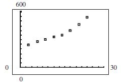
b. A quadratic model could be used.  2 47.70180240,870;axxx   2 0.072940.981544.45Axxx 

c. 2020 data: $63,676   10 a  $63,664–closer; 1061.564 A  ($61,564)

2050 data: 202.5 ($202,500) 40$189,292; a  40200.413 A  ($200,413–closer)

d. 150,000 a  when 32.5, x  in 2043; 150,000 A  when 31.9, x  in 2042

Chapter 2: Quadratic

and Other Special Functions

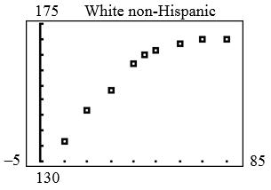
69. a.  0.7436.97Oxx

b.  0.2642.57Sxx

c.  0.7436.97 0.2642.57 x Fx x   This is called a rational function and measures the fraction of obese adults who are severely obese.

d. horizontal asymptote: 0.743 0.355. 0.264 y 

This means that if this model remains valid far into the future, then the long-term projection is that about 0.355, or 35.5%, of obese adults will be severely obese.

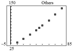
70. a. A quadratic function could be used to model each set of data.

2 0.009031.28124Wxxx 

2 0.006451.0220.0Oxxx  b. At  91.1,166.4xWxOx 

In 1970 + 92 = 2162, these population segments are predicted to be equal (at about 166.4 million each).

Chapter 2 Test _____________________________________________________________

c. h(x) = –1

Chapter 2: Quadratic and Other Special Functions

b. 3 ()(2)1fxx

d. () kxx 

2. figure b is the graph for b > 1. figure a is the graph for 0 < b < 1.

3. 2 () fxaxbxc  and a < 0 is a parabola opening downward. 4. a. 2 ()(1)1fxx

5. 322 ()4(4). fxxxxx 

a. and b. are the cubic choices. f(x) < 0 if 04 x  . Answer: b 6. 1 8if 0 ()4if 02 6if 2 xx x fxx xx

a. f(16) = 6 – 16 = –10 b. 11 (2)8(2)1622 f 

c. f(13) = 6 – 13 = –7

7. 2 if 1 () 4if 1 xx gx xx   

8. 2 ()214(7)(3) fxxxxx 

Vertex: (4) 2 22(1) b x a 

Point: (–2, 25)

Zeros: f(x) = 0 at x = –7 or 3.

Chapter 2: Quadratic and Other Special Functions

320940 (40)(10)1260 42 40103030 ff 

15. a. quartic b. cubic

16. a. f(x) = –0.3577x + 19.9227

9. 2 2 327 3720 (31)(2)0 xx xx xx 

3x – 1 = 0 or x – 2 = 0 1 , 2 3 x 

10. 2 2690 xx 63672663333 442 x

11. 2 2 111 23 3 3633 640 2(32)0 x xx xx xxx xx xx  

2 3 x  is the only solution.

12. 3(4) () 2 x gx x   Vertical asymptote at x = –2. g(4) = 0 Answer: c

13. 8 () 210 fx x 

Horizontal: 0 y 

Vertical: 2100 210 5 x x x   

b. f(40) = 5.6

c. f(x) = 0 if 19.9227 55.7 0.3577 x 

17. S: 1 30 6 pq

D: 30,000 20 p q  2 130,00030206 6 180180,000120 qq q qqq    

 2 300180,0000 (600)(300)0 qq qq  

E: 300 E: 503080 q p q p   18. 2 2 ()2850.9 ()15,000350.1 Rxxx Cxxx   a. 22 2 ()2850.9(15,000350.1) 25015,000 (100)(150) Pxxxxx xx xx    b. Maximum profit is at vertex. 250 125 2(1) x  Maximum profit = P(125) = $625 c. Break-even means P(x) = 0. From a., x = 100, 150.

19.

Chapter 2: Quadratic and Other Special Functions

a. Use middle rule for s = 15.

f(15) = –19.5 means that when the air temperature is 0ºF and the wind speed is 15 mph, then the air temperature feels like 19.5 ºF. In winter, the TV weather report usually gives the wind chill temperature.

b. f(48) = –31.4ºF

c. Break-even means P(x) = 0.

From a., x = 100, 150.

b. Linear: 14.1172yx

c. Linear: 

The cubic model is quite accurate, but both models are fairly close.

20.

Chapter 2: Quadratic and Other Special Functions

Chapter 2 Extended Applications & Group Projects ___________________________________

I. Body Mass Index (Modeling)

1. Eight points in the table correspond to a BMI of 30. Converting heights to inches, we have:

2. A linear model seems best as there appears to be roughly a constant rate of change of weight vs. height.

3. 5.700189.5yx

4. We note that  158.1 6l 1, b y  close to the actual value of 160 lb, and  22 2, 70.8 y  close to the actual value of 220 lb. The model seems to fit the data.

5. To test for obesity, substitute the person’s height in inches for x in the model, computing y. If the person’s weight is larger than y, then the person is considered obese. For a 5-foot-tall person,  15 0, 62.4 y  so 152.4 lb is the obesity threshold for someone who is 5 feet tall. For a 6-feet-2-inches-tall person,

23 4, 72.2 y  so 232.2 lb is the obesity threshold for someone who is 6 foot 2.

6. The Centers for Disease Control and Prevention (CDC) post the BMI formula

weight (lb)

height (in)

at their website (http://www.cdc.gov/healthyweight/assessing/bmi/adult_bmi/index.html, accessed March 12, 2019).

7. First solving the CDC formula for weight given a BMI of 30 gives

30height weight. 703

Chapter 2: Quadratic and Other Special Functions

II. Operating Leverage and Business Risk

1. Rxp 

2. a. 10010,000Cx

b. C is a linear function.

3. An equation that describes the break-even point is 10010,000xpx

4. a. 10010,000 10,000 100 xpx x p  

b. The solution is 4.a. is a rational function.

c. The domain is all real numbers, 100 p 

d. The domain in the context of this problem is 100 p 

5. a.

b. The function decreases as p increases.

6. A price of $1100 would increase the revenue for each unit but demand would decrease.

7. A price of $101 per unit would increase demand but perhaps such a demand could not be met.

8. a. Increasing fixed costs gives a higher operating leverage. Using modern equipment would give the higher operating leverage.

b. To find the break-even point with current costs we have 20010010,000 100. xx x  

To find the break-even point with modern equipment we have 2005030,000 200. xx x  

The higher the break-even point the greater the business risk. The cost with the modern equipment creates a higher business risk.

c. In this case, higher operating leverage and higher business event together. This higher risk might give greater profits for increases in sales. It might also give a greater loss of sales fall.