Chapter 2: Functions and Graphs
1 The points , , , E&ß#F&ß#G&ß# H&ß#I$ß!J!ß$ , , and are plotted in the figure.
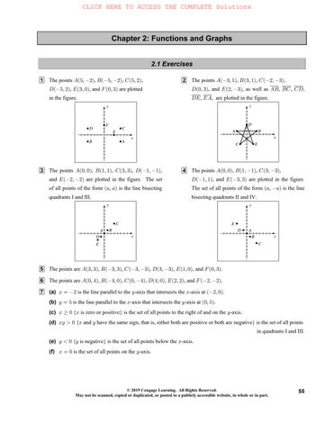
1 The points , , , E&ß#F&ß#G&ß# H&ß#I$ß!J!ß$ , , and are plotted in the figure.
2 The points , , , E$ß"F$ß"G#ß$ H!ß$I#ß$ EFFGGH , and , as well as , , , HIIE , , are plotted in the figure.
3 The points , , , , E!ß!F"ß"G$ß$H"ß" and are plotted in the figure. The set I#ß# of all points of the form , is the line bisecting ++ quadrants I and III.
4 The points , , , E!ß!F"ß"G$ß$ H"ß"I$ß$ , and are plotted in the figure. The set of all points of the form , is the line ++ bisecting quadrants II and IV.
5 The points are , , , , , and . E$ß$F$ß$G$ß$H$ß$I"ß!J!ß$
6 The points are , , , , , and . E!ß%F%ß!G!ß%H%ß!I#ß#J#ß#
7 is the line parallel to the -axis that intersects the -axis at . (a) Bœ# C B#ß!
(b) is the line parallel to the -axis that intersects the -axis at . Cœ& B C!ß&
(c) { is zero or positive} is the set of all points to the right of and on the -axis. B !B C
(d) { and have the same sign, that is, either both are positive or both are negative} is the set of all points BC!BC in quadrants I and III.
(e) { is negative} is the set of all points below the -axis.
C!C B
(f) is the set of all points on the -axis. Bœ! C
55 © 2019 Cengage Learning. All Rights Reserved. May not be scanned, copied or duplicated, or posted to a publicly accessible website, in whole or in part.
8 is the line parallel to the -axis that intersects the -axis at .
(a) Cœ# B C!ß#
(b) is the line parallel to the -axis that intersects the -axis at . Bœ% C B%ß!
(c) is the set of all points in quadrants II and IV{ and have opposite signs}. BÎC! BC
(d) is the set of all points on the -axis or -axis. BCœ! BC
(e) is the set of all points above the line parallel to the -axis which intersects the -axis at . C" B C!ß"
(f) is the set of all points on the -axis. Cœ! B
9 , (a) E%ß$F'ß#Ê.EßFœ'%#$œ%#&œ#*
EF
(b) , E%ß$F'ß#ÊQœßœ&ß %'$#" ###
10 , (a) E#ß&F%ß'Ê.EßFœ%#'&œ$'"#"œ"&(
(b) , E#ß&F%ß'ÊQœßœ"ß #%&'"
11 , (a) E(ß!F#ß%Ê.EßFœ#(%!œ#&"'œ%"
(b) , , E(ß!F#ß%ÊQœ (#!%*ßœ# ###
12 , (a) E&ß#F&ß#Ê.EßFœ&&##œ!"'œ%
(b) , E&ß#F&ß#ÊQœß œ&ß! &&## ##
##
13 , (a) E(ß$F$ß$Ê.EßFœ$($$œ"'!œ%
(b) , E(ß$F$ß$ÊQœß œ&ß$ ($$$ ##
##
14 , (a) E%ß(F!ß)Ê.EßFœ!%)(œ"'##&œ#%"
(b) , E%ß(F!ß)ÊQœß œ#ß %!() " ###
15 The points are , , and We need to show that the sides satisfy the Pythagorean theorem. E'ß$F"ß#G$ß#Þ
Finding the distances, we have , , and . Since is the .EßFœ&!.FßGœ$#.EßGœ)#.EßG largest of the three values, it must be the hypotenuse, hence, we need to check if . .EßGœ.EßF.FßG ###
Since , we know that is a right triangle. The area of a triangle is given )#œ&!$# ˜EFG ### by baseheight. We can use for the base and for the height. Eœ.FßG.EßF " # Hence, area œ,2œ$#&!œ%#&#œ#!#œ#! " """ # ###
16 The points are , , and E'ß$F$ß&G"ß&Þ
Show that ; that is, .EßFœ.EßG.FßG "%&œ#*""' ### ###
Area .œ,2œ†.EßG†.FßGœ#*""'œ#*##*œ#* "" " " ## # #
© 2019 Cengage Learning. All Rights Reserved. May not be scanned, copied or duplicated, or posted to a publicly accessible website, in whole or in part.
17 The points are , , , and We need to show that all four sides are the same E%ß#F"ß%G$ß"G#ß$Þ length. Checking, we find that , , . This guarantees that we have a .EßFœ.FßGœ.GHœ.HEœ#* rhombus {a parallelogram with equal sides}. Thus, we also need to show that adjacent sides meet at right angles. % This can be done by showing that two adjacent sides and a diagonal form a right triangle. Using , we see ˜EFG that and hence . We conclude that is a square. .EßGœ&).EßGœ.EßF.FßG EFGH
18 The points are , , , and E%ß"F!ß#G'ß"G#ß#Þ
Show that and , ..EßHœ.FßGœ%&.EßFœ.GHœ"(
19 Let , . . FœBCE$ß)ÊQœß$B)C ##
EF
Since , we must have and QœG&ß"! $B)Cœ&œ"!Ê ## EF
$Bœ#&)Cœ#"!ÊBœ"$Cœ#)Fœ"$ß#) and and . Thus, .
20 If is the midpoint of segment , then the midpoint of is the point that is three-fourths of the way from UEFUF E&ß)F'ß# to . UœQœßœ$Qœ ßœ &')#" "Î#'$#"$"
21 The perpendicular bisector of is the line that passes through the midpoint of segment and intersects EFEF segment at a right angle. The points on the perpendicular bisector are all equidistant from and . Thus, we EF EF need to show that , where , , and . Since each of these .EßGœ.FßGEœ%ß$Fœ'ß"Gœ$ß' distances is , we conclude that is on the perpendicular bisector of . &)GEF
22 Show that , where , , and . .EßGœ.FßGœ"#&Eœ$ß#Fœ&ß%Gœ(ß(
23 The points are , , and . We must have , , . E%ß$F'ß"TBßC.ETœ.FT B%C$œB'C"Ê ####
B)B"'C'C*œB"#B$'C#C"Ê #### {square both sides}
)B'C#&œ"#B#C$(Ê#!B)Cœ"#Ê&B#Cœ$
24 The points are , , and . We must have , , . E$ß#F&ß%TBßC.ETœ.FT B$C#œB&C%Ê ####
B'B*C%C%œB"!B#&C)C"'Ê #### {square both sides}
'B%C"$œ"!B)C%"Ê"'B"#Cœ#)Ê%B$Cœ(
25 Let represent the origin. Applying the distance formula with and , , we have S!ß! STBC .STœ&ÊB!C!œ&ÊBCœ& , . ## ##
This formula represents a circle of radius with center at the origin. &
26 , . This formula represents a circle of radius and center , . .GTœ<ÊB2C5œ< <25 ##
27 Let be an arbitrary point on the -axis. Applying the distance formula with and , we have U!ßCCUT&ß$ 'œ.TUÊ'œ!&C$Ê$'œ#&C'C*Ê , ## #
C'C#œ!ÊCœ$„""Ö × !ß$""!ß$"" # quadratic formula. The points are and
© 2019 Cengage Learning. All Rights Reserved. May not be scanned, copied or duplicated, or posted to a publicly accessible website, in whole or in part.
28 Let be an arbitrary point on the -axis. Applying the distance formula with and , we have U!ßCCUT"#ß% "$œ.TUÊ"$œ!"#C%Ê"'*œ"%%C)C"'Ê , ## #
C)C*œ!ÊC*C"œ!ÊCœ*" !ß*!ß" # , . The points are and .
29 Let , be an arbitrary point on the -axis. Applying the distance formula with and , we have UB!BUT#ß% &œ.TUÊ&ÊB#!%Ê#&œB%B%"'Ê , ## #
B%B&œ!ÊB&B"œ!ÊBœ&ß" "ß!&ß! # . The points are and .
30 Let , be an arbitrary point on the -axis. Applying the distance formula with and , we have UB!BUT"ß' (œ.TUÊ(ÊB"!'Ê%*œB#B"$'ÊB#B"#œ!Ê , ## ##
Bœ"„"$Ö × ""$ß!""$ß! quadratic formula. The points are and .
31 with points and .œ&#+ß+"ß$Ê&œ#+"+$Ê ##
#&œ%+%+"+'+*Ê&+"!+"&œ!Ê+#+$œ!Ê ### # +$+"œ!Ê+œ$" , . Since the -coordinate is negative in the third quadrant, , and , C+ œ " #+ + œ #ß "
32 with points and .œ$+ß+#ß"Ê$œ+#+"Ê ##
*œ+%+%+#+"Ê!œ#+#+%Ê++#œ!Ê+#+"œ!Ê ## ## +œ#ß" #ß#"ß" . The points are and .
##
33 With , and , we get , T+$U&ß#+.TU#'Ê&+#+$#'Ê
#&"!++%+"#+*#'Ê&+##+)!Ê&+#+%! ## # Interval Sign of Sign of
∞ßß%%ß∞ &+# +% ## && Resulting sign
From the sign chart, we see that or will assure us that , .++%.TU#' # &
34 With , and , we get , T+%U#ß+.TU"!Ê#++%"!Ê ##
%%+++)+"'"!Ê#+"#+"!!Ê+'+&!Ê+"+&! ## # # Interval Sign of Sign of ∞ß""ß&&ß∞ +" +& Resulting sign
From the sign chart, we see that or will assure us that , .+"+&.TU"!
35 Let be an arbitrary point on the -axis. , , , EBß!BU!ß#TBßCì.ETœ.UTÊ BBC!œB!C#ÊCœBC%C%ÊBœ%C% #### ####
© 2019 Cengage Learning. All Rights Reserved. May not be scanned, copied or duplicated, or posted to a publicly accessible website, in whole or in part.
36 Let be an arbitrary point on the -axis. , , , E!ßCCU'ß!TBßCì.ETœ.UTÊ
B!CCœB'C!ÊBœB"#B$'CÊCœ"#B$' #### ####
####
37 , , , , E#ß!F#ß!TBßCì.ET.FTœ&ÊB#CB#Cœ&Ê
B%B%Cœ&B%B%CÊ ####
B%B%Cœ#&"!B%B%CB%B%CÊ ## ## ##
"!B%B%Cœ#&)BÊ"!!B%B%Cœ'#&%!!B'%BÊ ## ###
"!!B%!!B%!!"!!Cœ'#&%!!B'%BÊ$'B"!!Cœ##& ### # # 38 , , , , E!ß"F!ß"TBßCì.ET.FTœ$ÊBC"BC"œ$Ê
####
BC#C"œ$BC#C"Ê ## ##
BC#C"œ*'BC#C"BC#C"Ê ## ## ##
'BC#C"œ*%CÊ$'BC#C"œ)"(#C"'CÊ ## ###
$'B$'C(#C$'œ)"(#C"'CÊ$'B#!Cœ%& ## ###
39 Let be the midpoint of the hypotenuse. Then , . Since , , we have QQœ+,Eœ+! "" ## .EßQœ++!,œ+,œ+,œ+,œ+,
In a similar fashion, show that , , . .FQœ.SQœ+, " # ##
40 Let , be the fourth vertex as shown in the figure.We need to show H+,- that the midpoint of is the same as the midpoint of . SHEG Qϧϧ!+!,-+,#### SH
and Qϧϧ!+-,+,#### GE
41 Plot the points , , , , and . E&ß$Þ&F#ß#G"ß!Þ&H%ß"I(ß#Þ& "!ß"!"!ß"! "#ß"#)ß) by by

)

42 Plot the points , , , , and . E"!ß%F(ß"Þ"G!ß'H$ß&Þ"I*ß#Þ"
© 2019 Cengage Learning. All Rights Reserved. May not be scanned, copied or duplicated, or posted to a publicly accessible website, in whole or in part.
43 Plot ,, ,, ,, and ,. (a)
"*)%ß)(!($"**$ß*)($'#!!$ß""$"#'#!!*ß""*#*'
(b) The number of U.S. households with a computer is increasing each year.
"*)#!"#)!$"!$)!$œ)!‚"! ß#$ß"#! by , EEEE{} $

")*&ß#!!&ß"!!ß$!!!ß"!!! by

44 Plot , , , , , and (a)
"*!!ß###'"*#!ß#!%#"*%!ß")()"*'!ß"('$"*)!ß"(%&#!!!ß"%)!
(b) Find the midpoint of and
"*#!ß#!%#"*%!ß")() ß œ"*$!ß"*'! "*#!"*%!#!%#")() ##
The midpoint formula predicts daily newspapers published in the year compared to the actual value "*'! "*$! of daily newspapers. "*%#
1 As in Example 1, we expect the graph of to be a line. Cœ#B$
Creating a table of values similar to those in the text, we have: B#"!"# C(&$""
By plotting these points and connecting them, we obtain the figure.
To find the -intercept, let in , and solve for to get .BCœ!Cœ#B$B"Þ&
To find the -intercept, let in , and solve for to get .CBœ!Cœ#B$C$ y x y x
2 gives the -intercept ; gives the -intercept Cœ%B#ìCœ!BBœ!C# " #
© 2019 Cengage Learning. All Rights Reserved. May not be scanned, copied or duplicated, or posted to a publicly accessible website, in whole or in part.
3 -intercept: -intercept:
CœB#ìBCœ!Ê!œB#ÊBœ#
Figure3Figure4
4 -intercept: ; -intercept: Cœ#B$ìBCœ!ÊBœ"Þ&CBœ!ÊCœ$
5 Multiplying the -values of by gives us all negative -values for . The vertex Cœ#BìCCœB#CCœ#B ## # of the parabola is at , so its -intercept is and its -intercept is . !ß!B!C!
x
Figure5Figure6
6 -intercept ; -intercept CœBìB!C! " $ #
7 -intercepts: , which Cœ#B"ìBCœ!Ê!œ#B"Ê"œ#BÊBœÊBœ„ ## # # "" ## can be written as or or ; -intercept: „„„#CBœ!ÊCœ" "" # # ##
Since we can substitute for in the equation and obtain an equivalent equation, we know the graph is BB symmetric with respect to the -axis. We will make use of this fact when constructing our table. As in Example 2, C we obtain a parabola.
B„#„„"„! C("" $" ## (" ## y x y x Figure7Figure8
8 -intercepts: ; -intercept CœB#ìBCœ!ÊBœ#ÊBœ„#C# ##
© 2019 Cengage Learning. All Rights Reserved. May not be scanned, copied or duplicated, or posted to a publicly accessible website, in whole or in part.
9
This graph is similar to the one in Example 5—multiplying by narrows the parabola . The BœCì BœC " " % % # # B!C! -intercept is and the -intercept is . y x y x Figure9Figure10
10 -intercept ; -intercept
Bœ#CìB!C! #
11 -intercept: ;BœC&ìBCœ!ÊBœ& #
CBœ!Ê!œC&ÊCœ&ÊCœ„& -intercepts: ##
Since we can substitute for in the equation and obtain an equivalent equation, we know the graph is symmetric CC with respect to the -axis. We will make use of this fact when constructing our table. As in Example 5, we obtain a B parabola.
B""%"%& C„%„$„#„"! y x y x Figure11Figure12
12 -intercept ; -intercepts: Bœ#C%ìB%CBœ!ÊCœ%ÊCœ„# ##
13 The graph is similar to the graph of in Example 6. The negative has the effect of “flipping”
CœBìCœB "" %% $$ the graph about the -axis. The -intercept is and the -intercept is .BB!C! y x y x Figure13Figure14
14 -intercept ; -intercept CœBìB!C! " # $
© 2019 Cengage Learning. All Rights Reserved. May not be scanned, copied or duplicated, or posted to a publicly accessible website, in whole or in part.
15 -intercept:
CœB)ìBCœ!Ê!œB)ÊBœ)ÊBœ)œ# $$$ $ CBœ!ÊCœ) -intercept: The effect of the is to shift the graph of down units. )CœB) $ B#"!"# C"'*)(! y x y x Figure15Figure16
16 -intercept: ; -intercept CœB"ìBCœ!ÊBœ"ÊBœ"œ"C" $$ $
17 -intercept ; -intercept This is the top half of the parabola . An equation of the bottom CœBìB!C!ÞBœC # half is .CœB y x y x
Figure17Figure18
18 The negative has the effect of “flipping” the graph of about the -axis. The -intercept is CœBìCœBCB! and the -intercept is .C!
19 -intercept: (not on graph) -intercept:
CœB%ìBCœ!Ê!œB%Ê%œBÊBœ"' CBœ!ÊCœ%
B!"%*"' C%$#"! y x y x Figure19Figure20
20 -intercept ; -intercept: None CœB%ìB%C
© 2019 Cengage Learning. All Rights Reserved. May not be scanned, copied or duplicated, or posted to a publicly accessible website, in whole or in part.
21 You may be able to do this exercise mentally. For example (using Exercise 1 with ), we see that Cœ#B$ substituting for gives us ; substituting for gives us or, equivalently, BBCœ#B$CCCœ#B$ Cœ#B$ BBCCCœ#B$ Cœ#B$ ; and substituting for and for gives us or, equivalently, . None of the resulting equations are equivalent to the original equation, so there is no symmetry with respect to the -axis,C B-axis, or the origin.
(a) The graphs of the equations in Exercises 5 and 7 are symmetric with respect to the -axis.C
(b) The graphs of the equations in Exercises 9 and 11 are symmetric with respect to the -axis.B
(c) The graph of the equation in Exercise 13 is symmetric with respect to the origin.
22 (a)(b)(c) 'ß)!ß""#"%
23 , , , (a) (b) (c) As As As BÄ"0BÄ BÄ#0BÄ BÄ$0BÄ –
24 , , , (a) (b) (c) As As As BÄ#0BÄ
(d) (e) As , As , BÄ∞0BÄ BÄ∞0BÄ
25 is a circle of radius with center at the origin.
26 is a circle of radius with center at the origin.
© 2019 Cengage Learning. All Rights Reserved. May not be scanned, copied or duplicated, or posted to a publicly accessible website, in whole or in part.
27 is a circle of radius with center . To determine the center from the B$C#œ*<œ*œ$G$ß# ## given equation, it may help to ask yourself “What values makes the expressions and equal to zero?” B$C# The answers are and .$# y x y x
Figure27Figure28
28 is a circle of radius with center . B$C#œ%<œ%œ#G$ß# ##
29 is a circle of radius with center . B$Cœ"'<œ"'œ%G$ß! # # y x y x
Figure29Figure30
30 is a circle of radius with center . BC#œ#&<œ#&œ&G!ß# # #
31 is a circle of radius with center . %B%Cœ"ÊBCœ<œœG!ß! #### """ %%# y x y x
Figure31Figure32
32 is a circle of radius with center . *B*Cœ%ÊBCœ<œœG!ß! #### %%# **$
© 2019 Cengage Learning. All Rights Reserved. May not be scanned, copied or duplicated, or posted to a publicly accessible website, in whole or in part.
33 As in Example 9, is the lower half of the circle .Cœ"'BBCœ"' # ## y x y x Figure33Figure34
34 is the upper half of the circle .Cœ%BBCœ% # ##
35 is the right half of the circle .Bœ*CBCœ* # ## y x y x Figure35Figure36
36 is the left half of the circle .Bœ#&CBCœ#& # ##
37 Center , radius G#ß$&ìB#C$œ&ÍB#C$œ#& #### #
38 Center , radius G&ß"$ìB&C"œ$ÍB&C"œ* #### #
""" %%% ## # # #
39 Center , , radius G!&ìBC!œ&ÍBCœ&
$#$#$# %$%$%$ #### #
40 Center , , radius G$#ìBCœ$#ÍBCœ")
41 An equation of a circle with center is . G%ß'B%C'œ< ## # Since the circle passes through , we know that and is one solution of the general equation. T$ß"Bœ$Cœ"
Letting and yields . An equation is .Bœ$Cœ"(&œ<Ê<œ(%B%C'œ(% ######
42 An equation of a circle with center at the origin is . BCœ< ###
Letting and yields . Bœ%Cœ(%(œ<Ê<œ'&BCœ'& ##### #
43 “Tangent to the -axis” means that the circle will intersect the -axis at exactly one point. The distance from the CC center to this point of tangency is units—this is the length of the radius of the circle.
G$ß'$
An equation is . B$C'œ* ##
44 “Tangent to the -axis” means that the circle will intersect the -axis at exactly one point. The distance from the CC center to this point of tangency is units—this is the length of the radius of the circle.
G&ß(&
An equation is . B&C(œ#& ##
© 2019 Cengage Learning. All Rights Reserved. May not be scanned, copied or duplicated, or posted to a publicly accessible website, in whole or in part.
45 The circle is tangent to the -axis and has center . BG%ß$
Its radius, , is the distance from the -axis to the -value of the center. An equation is $ BC
46 The circle is tangent to the -axis and has center . BG#ß)
##
Its radius, , is the distance from the -axis to the -value of the center. An equation is ) BC B#C)œ'%
47 Since the radius is and , is in QII, and . An equation is .#G252œ#5œ#B#C#œ% ##
48 Since the radius is and , is in QIV, and . An equation is $G252œ$5œ$B$C$œ* ##
49 The center of the circle is the midpoint of and . . The radius of the circle is QE%ß$F#ß(Qœ"ß# EF "" """ ## ### ## †.EßFœ%#$(œ$'"!!œ"$'œ%†$%œ$%
An equation is . B"C#œ$% ##
Alternatively, once we know the center, , we also know that the equation has the form "ß# B"C#œ<%B$C ## # . Now substitute for and for to obtain $&œ<Ê*#&œ<<œ$% #### # , or .
50 As in the solution to Exercise 49, and .Qœ"ß%<œ†.EßFœ)!œ#! EF "" ##
An equation is B"C%œ#! ##
51 complete the square on and BC%B'C$'œ!BCÊ ##
B%B%C'C*œ$'%*ÊB#C$œ%* ## ## This is a circle with center and radius .G#ß$<œ(
52 BC)B"!C$(œ!ÊB)B"'C"!C#&œ$("'#&Ê ## # #
B%C&œ%G%ß&<œ# ## . ;
53 complete the square on and BC%C(œ!BCÊBC%C%œ(%Ê ## ##
This is a circle with center and radius .
BC#œ"" G!ß#<œ"" # #
54 . ; BC"!B")œ!ÊB"!B#&Cœ")#&ÊB&Cœ(G&ß!<œ( ## # # # #
55 add to both sides and divide by #B#C"#B%C"&œ!"&#Ê ##
BC'B#Cœ BCÊ ## "& # complete the square on and
B'B*C#C"œ*"ÊB$C"œ ## "&$& ## ## .
This is a circle with center and radius .G$ß"<œ(! " #
56 %B%C"'B#%C$"œ!ÊBC%B'Cœ$"Ê ## ##
B%B%C'C*œ%*ÊB#C$œ G#ß$<œ#" ## $"#"" %%# ## . ;
57 BC%B#C&œ!ÊB%B%C#C"œ&%"Ê ## # # B#C"œ!G#ß"<œ! ## . ; (a point)
58 BC'B%C"$œ!ÊB'B*C%C%œ"$*%Ê ## # # B$C#œ!G$ß#<œ! ## . ; (a point)
59 BC#B)C#"œ!ÊB#B"C)C"'œ#"""'Ê ## # # B"C%œ%<% ## # . This is not a circle since cannot equal .
© 2019 Cengage Learning. All Rights Reserved. May not be scanned, copied or duplicated, or posted to a publicly accessible website, in whole or in part.
60 BC%B'C"'œ!ÊB%B%C'C*œ"'%*Ê ####
B#C$œ$<$ ## # . This is not a circle since cannot equal .
61 To obtain equations for the upper and lower halves, we solve the given equation for in terms of .CB
BCœ#&ÊCœ#&BÊCœ„#&B #### #
The upper half is and the lower half is . Cœ#&BCœ#&B ##
To obtain equations for the right and left halves, we solve the given equation for in terms of .BC
BCœ#&ÊBœ#&CÊBœ„#&C #### # .
The right half is and the left half is . Bœ#&CBœ#&C ##
B$Cœ'%ÊCœ'%B$ÊCœ„'%B$ ### ##
62 .
B$Cœ'%ÊB$œ'%CÊB$œ„'%CÊBœ$„'%C #### ## .
63 To obtain equations for the upper and lower halves, we solve the given equation for in terms of .CB
B#C"œ%*ÊC"œ%*B#ÊC"œ„%*B#Ê #####
Cœ"„%*B# #
The upper half is and the lower half is . Cœ"%*B#Cœ"%*B# ##
To obtain equations for the right and left halves, we solve the given equation for in terms of .BC
B#C"œ%*ÊB#œ%*C"ÊB#œ„%*C"Ê #####
Bœ#„%*C"Bœ#%*C"Bœ#%*C" ### . The right half is and the left half is .
64 B$C&œ%ÊC&œ%B$ÊC&œ„%B$Ê #####
Cœ&„%B$ #
B$C&œ%ÊB$œ%C&ÊB$œ„%C&Ê ##### Bœ$„%C& # .
65 From the figure, we see that the center of the circle is the origin, , and the radius is . Using the standard form !ß!& of an equation of a circle, , we have , B2C5œ<B!C!œ& ###### or {or use }.BCœ&#& ###
66 From the figure, we see that the center of the circle is the origin, , and the radius is . Using the standard form !ß!" of an equation of a circle, , we have , or {or use B2C5œ<B!C!œ"BCœ" ######### "}.
67 From the figure, we see that the diameter look at the -values of the rightmost and leftmost points of the circle is B "(œ))œ%25 units, so the radius is . The center , is at the average of the extreme values; that is, " # 2œœ$5œœ# ("#' ## , and similarly, . Using the standard form of an equation of a circle,
B2C5œ<B$C#œ%B$C#œ%"' ###### ### , we have , or {or use }.
68 diameter; radius; and œ%#œ'œ'œ$2œœ"5œœ# #%&" ## " #
An equation is , or {or use }.
B"C#œ$B"C#œ$* ######
© 2019 Cengage Learning. All Rights Reserved. May not be scanned, copied or duplicated, or posted to a publicly accessible website, in whole or in part.
69 The figure shows the lower semicircle of a circle centered at the origin having radius . The circle has equation % BCœ%C ### . We want the lower semicircle, so we must have -values, indicating that we should solve negative for and use the negative sign. , so is C BCœ%ÊCœ%BÊCœ„%BCœ%B ###### #### the desired equation.
70 , so is the desired equation since we BCœ$ÊBœ$CÊBœ„$CBœ$C ###### #### want -values. negative B
71 , so is the desired equation since we want
BCœ#ÊCœ#BÊCœ„#BCœ#B ###### #### positive -values.C
72 , so is the desired equation since we want
BCœ'ÊBœ'CÊBœ„'CBœ'C ###### #### positive -values.B
73 We need to determine if the distance from to is , , or and hence, will be TGT less than greater than equal to <<< insideoutsideon the circle, the circle, or the circle, respectively.
(a) , , {} is . T#ß$G%ß'Ê.TGœ%*œ"$<<œ%ÊTG inside (b) , , {} is . T%ß#G"ß#Ê.TGœ*"'œ&œ<<œ&ÊTG on (c) , , {} is . T$ß&G#ß"Ê.TGœ#&"'œ%"<<œ'ÊTG outside
74 , , {} is . (a) T$ß)G#ß%Ê.TGœ#&"%%œ"$œ<<œ"$ÊTG on (b) , , {} is . T#ß&G$ß(Ê.TGœ#&%œ#*<<œ'ÊTG inside
(c) , , {} is . T"ß#G'ß(Ê.TGœ#&#&œ&!<<œ(ÊTG outside
75 To find the -intercepts of , let and solve the resulting equation for . (a) BBC%B'C%œ!Cœ!B ## B%B%œ!ÊB#œ!ÊB#œ!ÊBœ# # #
(b) To find the -intercepts of , let and solve the resulting equation for . C BC%B'C%œ!Bœ! C ##
C'C%œ!ÊCœ œœ$„& '„$'"''„#& ## # .
76 (a) BC"!B%C"$œ!ìCœ!ÊB"!B"$œ!ÊBœ œ&„#$ "!„"!!&# # ## #
(b) BC"!B%C"$œ!ìBœ!ÊC%C"$œ!ÊCœ %„"'&# # ## #
The negative discriminant implies that there are no real solutions to the equation and hence, no -intercepts.C
77 . This is a circle with center and radius .BC%B'C%œ!ÍB#C$œ*G#ß$$ ## ## The circle we want has the same center, , and radius that is equal to the distance from to . G#ß$ GT#ß' .TGœ"'*œ& B#C$œ#& , , so an equation is . ##
78 By the Pythagorean theorem, the two stations are miles apart. The sum of their radii, .œ"!!)!¸"#)Þ!' ## )!&!œ"$! . , is greater than , indicating that the circles representing their broadcast ranges do overlap.
79 The equation of circle is . If we draw a line from the origin to the center of , we GB2C#œ# G # # ## # form a right triangle with hypotenuse { radius radius} and sides of length and . Thus, &#GGœ$#2 #" 2#œ$Ê2œ& ###
© 2019 Cengage Learning. All Rights Reserved. May not be scanned, copied or duplicated, or posted to a publicly accessible website, in whole or in part.
80 The equation of circle is . If we draw a line from the origin to the center of , we
GB2C$œ# G # # ## # form a right triangle with hypotenuse { radius radius} and sides of length and . Thus, &#GGœ($2 #"
2$œ(Ê2œ%! ### .
81 The graph of is the graph of to the left of and to the right of . Writing the -values in CCBœ$Bœ#B "# below interval notation gives us . ∞ß$∪#ß∞
Note that the -values play no role in writing the answer in interval notation. C
82 between and , so the interval is . CCBœ)Bœ))ß) "#
83 between and , excluding since at that value, so the interval is . CCBœ"Bœ"Bœ!CœC"ß!∪!ß" "# "#
84 to the left of , between and , and to the right of , so the interval notation is CCBœ)Bœ"Bœ"Bœ) "# ∞ß)∪"ß"∪)ß∞
85 The viewing rectangles significantly affect the shape of the circle. The second viewing rectangle results in a graph that most looks like a circle.
(1)
(2) by by #ß##ß# $ß$#ß#

(3)

(4) by by #ß#&ß& &ß&#ß#

86 From the graph, there are two –intercepts and two –intercepts (a) BC (b) Using the free–moving cursor, one can conclude that is BC& true whenever the point , is located inside the diamond shape. BC


87 Assign to Y. After trying a standard viewing rectangle, we see that the -intercepts are near BBBB $#*%$#% "!#&#& " the origin and we choose the viewing rectangle by . This is simply one choice, not necessarily the 'ß'%ß% best choice. For most graphing calculator exercises, we have selected viewing rectangles that are in a : $# proportion horizontal:vertical to maintain a true proportion. From the graph, there are three -intercepts. Use a B root feature to determine that they are , , and ."Þ#!Þ&"Þ'
© 2019 Cengage Learning. All Rights Reserved. May not be scanned, copied or duplicated, or posted to a publicly accessible website, in whole or in part.
by

by

88 From the graph, there are four -intercepts. They are approximately , and .B"Þ)!Þ(ß!Þ$"Þ$&
89 Make the assignments Y, Y, and YY. From the graph, there are two points of "#$# $ # œBBœ"Bœ intersection. They are approximately and . !Þ'ß!Þ)!Þ'ß!Þ)
$ß$#ß# by by


Figure89Figure90
90 Make the assignments Y, Y, and YY. From the graph, there are four points of "#$# % $ # # œ$Bœ"Bœ intersection. They are approximately and „!Þ*ß!Þ%„!Þ(ß!Þ(
91 Depending on the type of graphing utility used, you may need to solve for first. C BC"œ"ÊCœ"„"BBCœ"ÊCœ„"B # # # # && %% ## ; .
Make the assignments Y , YY, YY, Y , and YY. " #"$"% &% # & % # œ"Bœ"œ"œ"Bœ
Be sure to “turn off” Y before graphing. From the graph, there are two points of intersection. " They are approximately and !Þ***ß!Þ*')!Þ#&"ß!Þ!$#
$ß$#ß# $ß$#ß# by by


Figure91Figure92
92 ; B"C"œÊCœ"„B"BCœ"Ê ## # """" %%## ## Cœ„"B "" ## # . From the graph, there are two points of intersection. They are approximately and . !Þ(*ß"Þ%'"Þ%'ß!Þ(*
© 2019 Cengage Learning. All Rights Reserved. May not be scanned, copied or duplicated, or posted to a publicly accessible website, in whole or in part.
93 The cars are initially miles apart. The distance between them decreases to when they meet on the highway after %! #%% minutes. Then, the distance between them starts to increase until it is miles after a total of minutes.
!ß%!ß% !ß'!ß#!!!!ß&!!! by by ,


94 At noon on Sunday the pool is empty since when , . It is then filled with water, until at noon on Bœ!Eœ! Wednesday , it contains , gallons. It is then drained until at noon on Saturday , it is empty Bœ$")!!!Bœ' again.
95 °C ftsec. (a) @œ"!)( ìXœ#!Ê@œ"!)( ¸""#'Î X#($ #!#($ #($ #($ (b) Algebraically: @œ"!!!Ê"!!!œ"!)( Ê œÊ X#($X#($"!!! #($ #($"!)(
X#($"!!! #($†"!!! #($†"!!! #($"!)( "!)( "!)( œÊX#($œ ÊXœ #($¸%# ### ### °C.
Graphically: Graph Y and Y."# œ"!)(X#($Î#($œ"!!! At the point of their intersection, °C.X¸%# &!ß&!ß"!*!!ß"#!!ß"!! by

Figure95Figure96 "%ß"'*&ß"!& by

96 The horizontal lines and intersect the graph of at . Cœ**Cœ"!"Eœ$Î%==¸"&Þ"#ß"&Þ#( #
Thus, if , then "&Þ"#Ÿ=Ÿ"&Þ#(**ŸEŸ"!"
© 2019 Cengage Learning. All Rights Reserved. May not be scanned, copied or duplicated, or posted to a publicly accessible website, in whole or in part.
1 , E$ß#F&ß%Ê7œœœœ CC%#'$ BB&$)%
Figure1Figure2
2 , E%ß"F'ß$Ê7œœœœ
3 , {horizontal line}
E$ß%F'ß%Ê7œœœœ!
Figure3Figure4
4 , is undefined {vertical line}
E%ß$F%ß#Ê7œœœÊ7
5 , is undefined {vertical line}
E$ß#F$ß&Ê7œœœÊ7
Figure5Figure6
6 , {horizontal line}
E%ß#F$ß#Ê7œœœœ!
7 To show that the polygon is a parallelogram, we must show that the slopes of opposite sides are equal.
E#ß"F'ß$G%ß!H%ß#Ê7œœ77œœ7 , , , and . EF HE "$ %# HG GF
© 2019 Cengage Learning. All Rights Reserved. May not be scanned, copied or duplicated, or posted to a publicly accessible website, in whole or in part.
8 To show that the polygon is a trapezoid, we must show that the slopes of one pair of opposite sides are equal. E!ß$F$ß"G#ß'H)ß#Ê7œœ7 , , , . EF % $ GH
9 To show that the polygon is a rectangle, we must show that the slopes of opposite sides are equal parallel lines and the slopes of two adjacent sides are negative reciprocals perpendicular lines.
E'ß"&F""ß"#G"ß)H'ß&Ê7œœ77œœ7 , , , and . HE EF &$ $& GF HG
10 To show that the polygon is a right triangle, we must show that the slopes of two adjacent sides are negative reciprocals perpendicular lines. , , and .
E"ß%F'ß%G"&ß'Ê7œ7œ EF EG )& &)
11 is units to the left and units down from . The fourth vertex will have the same relative E"ß$&&F%ß#H position from , that is, units to the left and units down from . Its coordinates are G(ß&&&G (&ß&&œ"#ß! .
12 Let , , , and IœQœßJœQœßKœQœß BBCCBBCCBBCC ###### EF "#"##$#$$%$% FGGH LœQœßBBCC ## EH "%"%
. The slopes of opposite sides are equal or lines are vertical and 7œ 7œ7œ7œ CCCC BBBB IJKL JKIL $" %# $" %#
13 , , , Lines with equation pass through the origin. Draw lines through the origin with 7œ$#ìCœ7B #" $% slopes {rise, run}, {rise, run}, {rise, run}, and {rise, run}.$œ$œ"#œ#œ"œ#œ$œ"œ% #" $% A negative “rise” can be thought of as a “drop.” y x y 3x y s x y 2x y ~ x y x y 5x y q x y 3x y a x
Figure13Figure14
14 , , , 7œ&$ì "" #$
15 Draw lines through the point with slopes {rise, run}, {rise , run}, and T$ß"œ"œ#"œ"œ" " " # & {rise, run}.œ"œ&
Figure15Figure16
16 ; , , T#ß%7œ"#ì " #
© 2019 Cengage Learning. All Rights Reserved. May not be scanned, copied or duplicated, or posted to a publicly accessible website, in whole or in part.
17 From the figure, the slope of one of the lines is , so the slopes are . ? ? C&& B%% œ„
Using the point-slope form for the equation of a line with slope and point , , gives us 7œ„BCœ#$ & % "" C$œ„B#C$œ„B# && %% , or
18 , so the slopes are . 7œœ„ C$$ B%% ? ?
Using the point , gives us , or BCœ"ß#C#œ„B"C#œ„B" "" $$ %%
19 The line has slope and -intercept . The line has slope and -intercept .Cœ"B$"C$Cœ"B""C"
The line has slope and -intercept . Check your graph for parallel and perpendicular lines. Cœ"B""C" y x y x
20 , , Check your graph for parallel and perpendicular lines. Cœ#B"Cœ#B$CœB$ì " #
21 “Parallel to the -axis” implies the equation is of the form . (a) CBœ5
The -value of is , hence is the equation. BE$ß"$Bœ$
(b) “Perpendicular to the -axis” implies the equation is of the form . CC œ 5
The -value of is , hence is the equation. CE$ß""Cœ"
22 The line through and parallel to the -axis is . (a) E%ß#BCœ# (b) The line through and perpendicular to the -axis is . E%ß# BBœ%
23 Using the point-slope form, the equation of the line through with slope is E&ß$%
C$œ%B&ÊC$œ%B#!Ê%BCœ"(
24 Using the point-slope form, the equation of the line through with slope is E"ß% # & C%œB"Ê&C%œ#B"Ê&C#!œ#B#Ê#B&Cœ## # &
25 ; slope {use the point-slope form of a line} E%ß"Ê " $
C"œB%Ê$C"œ"B%Ê$C$œB%ÊB$Cœ( " $
26 ; slope .E!ß#&ÊC#œ&B!ÊC#œ&BÊ&BCœ#
27 , . By the point-slope form, with , an equation of the line is E%ß&F$ß'Ê7œE%ß& EF "" (
C&œB%Ê(C&œ""B%Ê(C$&œ""B%%Ê""B(Cœ* "" (
28 , . By the point-slope form, with , an equation of the line is E$ß#F%ß%Ê7œE$ß# EF ' (
C#œB$Ê(C#œ'B$Ê(C"%œ'B")Ê'B(Cœ% ' (
© 2019 Cengage Learning. All Rights Reserved. May not be scanned, copied or duplicated, or posted to a publicly accessible website, in whole or in part.
29 , -intercept Use the slope-intercept form with to get . The slope of the line E$ß&C#ì,œ#Cœ7B# through and is . .E$ß&F!ß#CœB#Ê$Cœ(B'Ê(B$Cœ' (( $$
30 , -intercept Use the slope-intercept form with to get . The slope of the line through E"ß)C&ì,œ&Cœ7B& E"ß)F!ß&$Cœ$B&Ê$BCœ& and is . .
31 , . .E#ß"!F$ß!Ê7œ#C!œ#B$ÊCœ#B'Ê#BCœ' EF
32 , . .E"ß'F&ß!Ê7œ"C!œ"B&ÊCœB&ÊBCœ& EF
33 . Using the same slope, , with , gives us &B#Cœ%Í&B%œ#CÍCœB#E$ß" && ##
C"œB$Ê#C"œ&B$Ê#C#œ&B"&Ê&B#Cœ"( & #
34 . Using the same slope, , with , gives us B$Cœ"Í$CœB"ÍCœBE$ß& """ $$$
C&œB$Ê$C"&œB$ÊB$Cœ"# " $ .
35 . The slope of this line is , so we’ll use the negative #B&Cœ)Í#B)œ&CÍCœB#)# &&& reciprocal, , for the slope of the new line, with . E(ß$ & #
C$œB(Ê#C$œ&B(Ê#C'œ&B$&Ê&B#Cœ#* & # .
36 . Using the negative reciprocal of for the slope, with , $B#Cœ(ÍCœBE&ß% $($ ###
C%œB&Ê$C"#œ#B"!Ê#B$Cœ# # $
37 , . E%ß!F!ß$Ê7œ EF $ %
Since is the -intercept, we use the slope-intercept form with to get .FC,œ$CœB$ $ %
38 , . Using the slope-intercept form with gives us .E'ß!F!ß"Ê7œ,œ"CœB" EF " " ' '
39 , . By the point-slope form, with , an equation of the line is
E&ß#F"ß%Ê7œE&ß# EF " $ C#œB&ÊCœB#ÊCœB ""&""" $$$$$ .
40 , . By the point-slope form, with , an equation of the line is E$ß"F#ß(Ê7œE$ß" EF ' & C"œB$ÊCœB"ÊCœB ''")'#$ &&&&& .
41 We need the line through the midpoint of segment that is perpendicular to segment . QEFEF E$ß"F#ß'ÊQœ7œQ7œ , , and . Use and in the point-slope form. EFEFEF "&(& ##&(
CœBÊ(Cœ&BÊ(Cœ&BÊ&B(Cœ"& &&"&"$&& #(#####
E%ß#F#ß'ÊQœ"ß#7œQ7œ EFEFEF %$ $%
42 , and . Use and in the point-slope form.
C#œB"Ê%C)œ$B$Ê$B%Cœ& $ %
43 An equation of the line with slope through the origin is , or "C!œ"B!CœB
44 An equation of the line with slope through the origin is , or ."C!œ"B!CœB
© 2019 Cengage Learning. All Rights Reserved. May not be scanned, copied or duplicated, or posted to a publicly accessible website, in whole or in part.
45 We can solve the given equation for to obtain the slope-intercept form, . CCœ7B, #Bœ"&$CÊ$Cœ#B"&ÊCœB&7œ,œ& ; , ## $$
46 ; , (Bœ%C)Ê%Cœ(B)ÊCœB#7œ,œ# (( %%
47 ; , %B$Cœ*Ê$Cœ%B*ÊCœB$7œ,œ$ %% $$
48 ; , B&Cœ"&Ê&CœB"&ÊCœB$7œ,œ$ "" &&
49 An equation of the horizontal line with -intercept is . (a) C$Cœ$
(b) An equation of the line through the origin with slope is .CœB "" ##
(c) An equation of the line with slope and -intercept is .C"CœB" $$ ##
(d) An equation of the line through with slope is $ß# "C#œB$
Alternatively, we have a slope of and a -intercept of , i.e., . "C "CœB"
50 An equation of the vertical line with -intercept is . (a) B#Bœ#
(b) An equation of the line through the origin with slope is.%% $$CœB
(c) An equation of the line with slope and -intercept is . "" $$C#CœB#
(d) An equation of the line through with slope is . #ß& $C&œ$B#
Alternatively, we have a slope of and a -intercept of , i.e., $C"Cœ$B"
51 Since we want to obtain a “” on the right side of the equation, we will divide each term by .""! &B#C"!BC "!"!"!#&œÍœ"B#C& . The -intercept is and the -intercept is .
52 Since we want to obtain a “” on the right side of the equation, we will divide each term by .""# %B$C"#BC "#"#"#$%œÍœ"B$C% . The -intercept is and the -intercept is .
© 2019 Cengage Learning. All Rights Reserved. May not be scanned, copied or duplicated, or posted to a publicly accessible website, in whole or in part.
53 Since we want to obtain a “” on the right side of the equation, we will divide each term by ."' %B#C'#BC BC '''$$ $ œÍœ"Íœ"B C$ . The -intercept is and the -intercept is . $ # $ #
54 . The -intercept is and the -intercept is . B$C#BC ####œÍœ"B#C # $ # $
55 The radius of the circle is the vertical distance from the center of the circle to the line , that is, Cœ& <œ&#œ(G$ß#B$C#œ%* . With , an equation is . ##
56 The line through the origin and is perpendicular to the desired line. T This line has equation , so the desired line has slope . CœB %$ $% With , an equation is T$ß% C%œB$ÊCœB%ÊCœB $$
57 The -intercept is (in millions of dollars), so when no widgets are produced, production costs are $1 million. The C" slope is shown as positive , with the in thousands, so for every widgets produced, production costs increase " $ $ $!!! $1 million.
58 The -intercept is (in gallons of gas remaining), so after filling the gas tank and driving 0 miles, the driver has C"& "& gallons in the tank. The slope is shown as , so for every miles driven, the number of gallons remaining in #' " #' the tank decreases gallon. "
59 The -intercept of the graph of the equation is , which has no meaning since the length (a) PPœ"Þ&$>'Þ('Þ( cannot be negative. When , cm, which is the shortest length for which this >œ"#Pœ"Þ&$"#'Þ(œ""Þ'' model applies.
(b) The slope is , so for every increase of week in time, there is an increase of cm in length. "Þ&$ " "Þ&$ (c) , or approximately weeks. Pœ#)Ê"Þ&$>'Þ(œ#)Ê>œ¸##Þ') #$ #)'Þ( "Þ&$
60 . Wœ!!$"Þ)!&GìWœ!Þ$&Ê!!$"Þ)!&Gœ!Þ$&ÊGœ¸!Þ"(( !Þ$&!!$ "Þ)!&
61 The -intercept of the graph of the equation is , which has no meaning since the (a) [[œ"Þ(!P%#Þ)%#Þ) weight cannot be negative. When , tons, which is the smallest weight for Pœ$

Figure79Figure80
80 and . Assign to Y and B"!Cœ"#$ÍCœB"#$Î"!#BCœ'ÍCœ#B'B"#$Î"! " Cœ#B'$ß"# to Y. Similarly to Exercise 79, the lines intersect at . #
81 From the graph, we can see that the points of intersection are , , and . The lines E!Þ)ß!Þ'F%Þ)ß$Þ%G#ß& intersecting at are perpendicular since they have slopes of and . Since and E#.EßFœ$*Þ# " # .EßGœ$*Þ# , the triangle is isosceles. Thus, the polygon is a right isosceles triangle.
"&"!&ß"!ß"$ß$#ß# by

by

82 The equations of the lines can be rewritten as , , , and CœB!Þ"(Cœ%Þ#B"Þ*CœB"Þ$ "" %Þ#%Þ# Cœ%Þ#B$Þ& E!Þ(&ß!Þ$& . From the graph, we can see that the points of intersection are approximately , F"Þ!)ß"Þ!%G!Þ"%ß"Þ$$H!Þ%(ß!!&* , , and .. The first and third lines are parallel as are the second and fourth lines. In addition, these pairs of lines are perpendicular to each other since their slopes are and . %Þ# " %Þ# Since and , it is not a square. Thus, the polygon is a rectangle. .EßF¸"Þ%$.EßH¸"Þ#&
83 The data appear to be linear. Using the two arbitrary points and , the slope of the line is !Þ'ß"Þ$%Þ'ß)Þ& )Þ&"Þ$ %Þ'!Þ' œ"Þ)C"Þ$œ"Þ)B!Þ'ÊCœ"Þ)B!Þ## . An equation of the line is .
If we find the regression line on a calculator, we get the model .C¸"Þ)%&)*B!Þ#"!#( !!!! ß&ß"!ß&ß$Þ& by by Figure83Figure84


84 The data appear to be linear. Using the two arbitrary points and , the slope of the line is !Þ%ß#Þ))%Þ%ß!Þ') !Þ')#Þ))
%Þ%!Þ% œ!Þ&&C#Þ))œ!Þ&&B!Þ%ÊCœ!Þ&&B$Þ" . An equation of the line is .
If we find the regression line on a calculator, we get the model .C¸!Þ&%*&"B$Þ!*'#"
© 2019 Cengage Learning. All Rights Reserved. May not be scanned, copied or duplicated, or posted to a publicly accessible website, in whole or in part.
85 Plot the points with the form Year, Distance: , , , , and (a)
"*""ß"&Þ&#"*$#ß"&Þ(#"*&&ß"'Þ&'"*(&ß"(Þ)* "**&ß")Þ#*
(b) To find a first approximation for the line use the arbitrary points and . The "*""ß"&Þ&#"**&ß")Þ#* resulting line is . Adjustments may be made to this equation. If we find the regression H¸!Þ!$$]%(Þ&%& " line on a calculator, we get the model .H¸!Þ!$'%)]&%Þ%(%!*
(c) Using from part (b), when , so the distance is . meters—almost equal to the H Bœ"*)&Cœ"(Þ*' "(*' " actual record of meters. "(Þ*( "*!!"!"&"*!!"!#"'! !ß#!ß#ß#! !ß#!ß#!ß#!ß" by by


86 For an approximation for the line, we’ll use the first and last points given; that is, and (b) "*"$ß#&%Þ%
"***ß##$Þ" X#&%Þ%œ ]"*"$Ê ##$Þ"#&%Þ% "***"*"$ . These points determine the line
X¸!Þ$'$*&]*&!Þ'%$ C¸!Þ$(%&&B*(!Þ&)#'# . The regression line is (c) seconds, which is off by seconds. Xœ!Þ$'$*&"*)&*&!Þ'%$¸##)Þ# "Þ* (d) The slope of the line is approximately . This means that , the record time for the mile has !Þ% on the average decreased by secyr.!Þ%Î
1 , , and .0BœBB%Ê0#œ%#%œ'0!œ%0%œ"'%%œ#% #
2 , , and .0BœBB$Ê0$œ#(*$œ#"0!œ$0#œ)%$œ* $#
3 is undefined for the real numbers.
0BœB#$BÊ0"œ"#$"œ"$
Similarly, 0'œ'#$'œ%")œ#")œ#! and .0""œ""#$""œ*$$œ$$$œ$'
Note that , for any , would be undefined. 0++#
4 0BœB$BÊ0"œ"$"œ"%œ"#œ$
Similarly, 0#œ#$#œ#"œ#"œ" and is undefined for the real numbers. 0&œ&$&œ&#
Note that , for any , would be undefined. 0++$
5 , , and is undefined. 0BœÊ0#œœ0!œœ!0$œ B# #!$ B$ &&$ !
6 is undefined, , and 0BœÊ0#œ 0!œœ!0#œœ" #B % ! % B# ! # %
7 (a) (b) 0Bœ&B#Ê0+œ&+#œ&+#0+œ&+#œ&+# (c) (d) 0+œ"†&+#œ&+# 0+2œ&+2#œ&+&2#
© 2019 Cengage Learning. All Rights Reserved. May not be scanned, copied or duplicated, or posted to a publicly accessible website, in whole or in part.
(e) 0+02œ&+#&2#œ&+&2%
(f) Using parts (d) and (a), 0+20+&+&2#&+#&2 222 œœ œ &
8 (a)(b) 0Bœ"%BÊ0+œ"%+œ"%+0+œ"%+œ"%+ (c) (d) 0+œ"†"%+œ%+" 0+2œ"%+2œ"%+%2
(e) 0+02œ"%+"%2œ#%+%2
(f) Using parts (d) and (a), . 0+20+"%+%2"%+%2 222 œœ œ %
9 (a) 0BœB$Ê0+œ+$œ+$ ## #
(b) (c) 0+œ+$œ+$ 0+œ"†+$œ+$ # ###
(d) 0+2œ+2$œ+#+22$œ+#+22$ # ####
(e) 0+02œ+$2$œ+2' ####
(f) 0+20++#+22$+$#+222#+2 2222 œœœœ#+2 ####
10 (a)(b) 0Bœ$BÊ0+œ$+œ$+0+œ$+œ$+ ### ##
(c) 0+œ"†$+œ$+ ##
(d) 0+2œ$+2œ$+#+22œ$+#+22 # ####
(e) 0+02œ$+$2œ'+2 ####
(f) 0+20+$+#+22$+#+222#+2 2222 œœœœ#+2 ####
11 (a) 0BœBB$Ê0+œ++$œ++$ ## #
(b) (c) 0+œ++$œ++$ 0+œ"†++$œ++$ # ###
(d) 0+2œ+2+2$œ+#+22+2$ # ##
(e) 0+02œ++$22$œ+2+2' ### #
(f) 0+20++#+22+2$++$#+2222#+2" 2222 œœœ œ#+2" ### #
12
(a) 0Bœ#B$B(Ê0+œ#+$+(œ#+$+( ## #
(b) 0 +œ#+$+(œ#+$+( # #
(c) 0+œ"†#+$+(œ#+$+( ##
(d) 0+2œ#+2$+2(œ#+#+22$+$2(œ # ## #+%+2#2$+$2( ##
(e) 0+02œ#+$+(#2$2(œ#+#2$+$2"% ### #
(f) 0+20+#+%+2#2$+$2(#+$+( 22 œ
## # #
œœœ%+#2$ %+2#2$22%+#2$ 22
© 2019 Cengage Learning. All Rights Reserved. May not be scanned, copied or duplicated, or posted to a publicly accessible website, in whole or in part.
# # ### #
13 (a) (b) 1Bœ%BÊ1œ%œ%†œ1+œ%+Êœ """% "" ++++ 1+%+
# #
(c) (d) since 1+œ%+œ%+ 1+œ%+œ#+œ#++!
14 (a) (b) 1B œ#B(Ê1œ#(œ(œ œœ ""##(+""" ++++ 1+#+(#+(
15 (a) 1BœÊ1œœ†œœ #B "#"Î+#Î++#+#+ B"+ "Î+"+"++"
# # # (d) , or,
17 All vertical lines intersect the graph in at most one point, so the graph the graph of a function because it passes the Vertical Line Test. is
18 At least one vertical line intersects the graph in more than one point, so the graph the graph of a function because it fails the Vertical Line Test. is not
19 The domain is the set of -values; that is, . Note that the solid dots on the figure correspond HBHœ%ß"∪Ò#ß%Ñ to using brackets {including}, whereas the open dot corresponds to using parentheses {excluding}. The range is V the set of -values; that is, .CVœÒ$ß$Ñ
20 Domain {-values}. Range {-values}. HœBœÒ%ß%ÑVœCœ$ß"∪"ß$
21 The domain of a function is the set of all -values for which the function is defined. In this case, the graph (a) 0B extends from to . Hence, the domain is . Bœ$Bœ%$ß%
(b) The range of a function is the set of all -values that the function takes on. In this case, the graph includes all 0C values from to . Hence, the range is . Cœ#Cœ# #ß#
(c) is the -value of corresponding to . In this case, . 0"C0 Bœ" 0"œ!
(d) If we were to draw the horizontal line on the same coordinate plane, it would intersect the graph at Cœ" Bœ"#0Bœ"ÊBœ"# , , and . Hence, , , and . "" ##
(e) The function is above between and , and also to the right of . Hence, "Bœ"Bœ Bœ# " # 0B"ÊB−"ß∪Ð#ß%Ó " #
© 2019 Cengage Learning. All Rights Reserved. May not be scanned, copied or duplicated, or posted to a publicly accessible website, in whole or in part.
22 (a)(b) (c) 0"œ" &ß("ß#
(d)(e) 0Bœ"ÊBœ$ß0B"ÊB−$ß"∪ "ß$ß&$ß&
Note: In Exercises 23–0, we need to make sure that the radicand {the expression under the radical sign} is greater than or equal to zero and that the denominator is not equal to zero.
23 0Bœ#B(ì#B( !Ê#B (ÊB Íß∞ (( ##
24 0Bœ%$Bì%$B !Ê% $BÊBŸÍ∞ß %% $$
25 0Bœ"'Bì"'B !Ê"' BÊBŸ"'ÊBŸ%Ê # ### %ŸBŸ%%ß% , or in interval notation.
26 or 0BœB#&ìB#& !ÊB &ÊB &BŸ&ÍÐ∞ß&Ó∪Ò&ß∞Ñ # #
27 or , 0Bœ%B*ì%B* !ÊB ÊB ÊB BŸ # ## *$$$ %### or in interval notation. ∞ß∪ß∞ $$ ##
28 0Bœ"'#&Bì"'#&B !Ê"' #&BÊ#&BŸ"'ÊBŸÊBŸÊ # #### "'% #&& ŸBŸß %%%% &&&& , or in interval notation.
29 For this function we must have the denominator not equal to . The denominator is 0Bœì! B" B*B $ B*BœBB*œBB$B$BÁ!ß$ß$!ß$ß$ $#, so . The solution is then all real numbers . In except interval notation, we have . We could also denote this solution as ∞ß$∪$ß!∪!ß$∪$ß∞ ‘ „$ß!{}.
30 , 0Bœì'B"$B&œ!Ê#B&$B"œ!Ê %B 'B"$B& # # &" #$ ‘
31 For this function we must have the radicand greater than or equal to the 0Bœì ! #B& B&B% # and denominator not equal to . The radicand is greater than or equal to if , or, equivalently, . The !!#B& !B & # denominator is , so . The solution is then all real numbers greater than or equal to , B"B%BÁ"ß% & # excluding . In interval notation, we have . %ß%∪%ß∞ & #
32 ;0BœìB%œ!ÊB#B#œ!ÊBœ„# %B$ B% # #
%B$ !ÊB #∪#ß∞ , so the domain is , $$ %%
33 For this function we must have .0BœìB#!ÊB# B% B#
Note that “” must be used since the denominator cannot . In interval notation, we have . !#ß∞ equal
34 , so the domain is 0BœìB$!ÊB$BÁ$$ß$∪$ß∞ " B$B$
35 We must have and .0BœB$$BìB$ !ÊB $$B !ÊBŸ$
The domain is the intersection of and , that is, . B $BŸ$$ß$
© 2019 Cengage Learning. All Rights Reserved. May not be scanned, copied or duplicated, or posted to a publicly accessible website, in whole or in part.
36 We must have and .0Bœ"BB&ì"B !ÊBŸ"B& !ÊB &
The domain is the intersection of and , that is, . BŸ"B &&ß"
37 {see the sign chart} or .0BœB#B'ìB#B' !ÊBŸ#B '
Interval Sign of Sign of
∞ß##ß''ß∞ B# B' Resulting sign
In interval notation, we have .Ð∞ß#Ó∪Ò'ß∞Ñ
38 or {use a sign chart}
0BœB#B%ìB#B% !ÊBŸ%B#Ê Ð∞ß%Ó∪Ò#ß∞Ñ
39 {-values}; {-values}{}. (a) HœBœÒ&ß$Ñ∪Ð"ß"Ó∪Ð#ß%ÓVœCœ$∪"ß%
Note that the notation for including the single value in uses braces. $V (b) on an interval if it goes up as we move from left to right, 0 is increasing so is increasing on 0 Ò%ß$Ñ∪$ß% 0 is decreasing on an interval if it goes down as we move from left to right, so is decreasing on 0 &ß%∪Ð#ß$Ó Bœ%Bœ$ . Note that the values and are in intervals that are listed as increasing and in intervals that are listed as decreasing. 0 is constant on an interval if the -values do not change, so is constant on . C 0 Ð"ß"Ó
40 -values ; -values (a) HœBœÒ&ß$Ñ∪Ð#ß"Ó∪!ß#Ñ∪Ð$ß&ÓVœCœ$ß$∪% (b) is increasing on . is decreasing on . is constant on 0 Ò&ß$Ñ∪Ð$ß%Ó0 Ò!ß#Ñ0 Ð#ß"Ó∪%ß&
41 The graph of the function is increasing on and is decreasing on , so there must be a high point at Ð∞ß$Ó$ß# Bœ$Ò#ß∞ÑBœ# . Now the graph of the function is increasing on , so there must be a low point at .
42 The graph of the function is decreasing on and , and is increasing on and .Ð∞ß#Ó"ß%#ß"Ò%ß∞Ñ
© 2019 Cengage Learning. All Rights Reserved. May not be scanned, copied or duplicated, or posted to a publicly accessible website, in whole or in part.
43 This is a line with slope and -intercept . (a) 0Bœ#B"ì #C"
(b) The domain and the range are equal to . HV∞ß ∞
(c) is decreasing on its entire domain, that is, . 0 ∞ß∞
44 This is a line with slope and -intercept . (a) 0Bœ#B"ì #C"
(b) , Hœ∞ß∞Vœ∞ß∞
(c) Increasing on ∞ß∞
45 To sketch the graph of , we can make use of the symmetry with respect to the -axis. (a) 0Bœ%BC # B„%„$„#„"!
(b) Since we can substitute any number for , the domain is all real numbers, that is, . By examining the BH œ ‘ figure, we see that the values of are at most . Hence, the range of is all reals less than or equal to , that is, C%0 % VœÐ∞ß%Ó
(c) A common mistake is to confuse the function values, the ’s, with the input values, the ’s. We are not CB interested in the specific -values for determining if the function is increasing, decreasing, or constant. We are C only interested if the -values are going up, going down, or staying the same. For the function , C0 B œ % B # we say since the -values are getting larger as we move from left to right over the 0Ð ∞ß !ÓC is increasing on B ∞!0 Ò!ß∞ÑC -values from to . Also, since the -values are getting smaller as we move is decreasing on from left to right over the -values from to . Note that this answer would have been the same if the B!∞ function was , , or any function of the form , where is any 0Bœ&!!B0Bœ$!!B 0Bœ+B+ ## # real number. y x y x
© 2019 Cengage Learning. All Rights Reserved. May not be scanned, copied or duplicated, or posted to a publicly accessible website, in whole or in part.
46 , (a) (b) 0BœB"ì Hœ∞ß∞VœÒ"ß∞Ñ #
(c) Decreasing on , increasing on Ð∞ß!Ó Ò!ß∞Ñ
47 This is half of a parabola opening to the right. It has an -intercept of and no (a) 0BœB"ì B " C-intercept.
(b) , so the domain is . B" !ÊB " HœÒ"ß∞Ñ
The -values are all positive or zero, so the range is . CV œ Ò!ß ∞Ñ (c) is increasing on its entire domain, that is, on . 0Ò"ß ∞Ñ y x y x
Figure47Figure48
#
48 , Decreasing on (a) (b) (c) 0BœB"ìHœÐ∞ß%ÓVœÒ!ß∞Ñ Ð∞ß%Ó
49 This is a horizontal line with -intercept . (a) 0Bœ%ì C%
(b) The domain is and the range consists of a single value, so . Hœ∞ß∞ Vœ% (c) is constant on its entire domain, that is, . 0 ∞ß∞ y x y x
Figure49Figure50
50 , Constant on (a) (b) (c) 0Bœ$ìHœ∞ß∞Vœ$ ∞ß∞
51 We recognize as the lower half of the circle (a) Cœ0Bœ$'B BCœ$' # ##
(b) To find the domain, we solve . . $'B !$'B !ÊBŸ$'ÊBŸ'ÊHœ'ß' ###
From the figure, we see that the -values vary from to . Hence, the range is . C Cœ'Cœ! V'ß!
(c) As we move from left to right, for to , the -values are decreasing. From to , the - Bœ'Bœ!C Bœ!Bœ'C values increase. Hence, is decreasing on and increasing on . 0'ß !!ß '
© 2019 Cengage Learning. All Rights Reserved. May not be scanned, copied or duplicated, or posted to a publicly accessible website, in whole or in part.
53 , so .0BœB'B0#œ#'#œ%"#œ) ##
0 #20# %%22"#'2)2#222# 2222 2 œœœ
54 , so .0Bœ#B&0#œ##&œ#†%&œ)&œ$ # # 0#20# #%%22&$))2#2) 2222
0B20B%B%B%2%2% 222B2B2BB22BB2 œœœœœ
56 0B20BBB#B22 222 œœœ ""BB2 B2B2B B 2BB2
#B222#B2#B2 2BB22BB2BB2
57 0B0+B$+$B$+$B$+$ B+B+B+
œœœ B$+$B+" B+B$+$B+B$+$ B$+$
B$+$
58 0B0+B#+#B+B+B+B+ B+B+B+B+ œœœœB+B+ $$$$## ##
59 As in Example 7, and has the form . +œœ00BœB, #""" $$''
0$œ$,œ,0$œ#,œ#Ê,œ0BœB "" " $"$ '# # #'# . But , so , and .
60 As in Example 7, and has the form . +œœœ00BœB, #(*$$ %#'##
0#œ#,œ$,0#œ($,œ(Ê,œ%0BœB% $ $ # # . But , so , and
© 2019 Cengage Learning. All Rights Reserved. May not be scanned, copied or duplicated, or posted to a publicly accessible website, in whole or in part.
Note: For Exercises 61–70, a good question to consider is, “Given a particular value of , can a unique value of be BC found?” If the answer is yes, the value of (general formula) is given. If not, two ordered pairs satisfying the C relation having in the first position are given. B
$CœB(ÊCœ B( $ # #
61 , which is a function
62 , which is a function
Bœ$C#ÊB#œ$CÊCœ B# $
63 , not a function: BCœ%ÊCœ%BÊCœ„%B!ß„# #### #
64 , not a function: CBœ%ÊCœ%BÊCœ„%B!ß„# #### #
65 is a function since for any , , is the only ordered pair in having in the first position. Cœ&BB&[B
66 is not a function: and Bœ$$ß!$ß"
67 Any ordered pair with -coordinate satisfies . Two such ordered pairs are and . Not a function B!BCœ!!ß!!ß"
68 , which is a function BCœ!ÊCœB
69 , not a function: CœBÊ„Cœ„BÊCœ„B"ß„"
70 Many ordered pairs with -coordinate or any other number satisfy .B$CB
Two such ordered pairs are and . Not a function $ß"$ß#
71 Zœ6A2œ$!BB#!BBB œ$!#B#!#BBœ#"&B†#"!BBœ%B"&B"!B
72 Wœ#<2##<œ#<"!%<œ#!<%<œ%<&< 1111111 ###
73 The formula for the area of a rectangle is {Arealengthwidth} (a) Eœ6Aœ‚ Eœ&!!ÊBCœ&!!ÊCœ &!! B (b) We need to determine the number of linear feet first. There are two walls of length , two walls of length TC
B$BTœœB#C#B$œ$B#' &!! B , and one wall of length , so Linear feet of wall. The cost is times , so . , G"!!TGœ"!!Tœ$!!B'!! "!!!!! B
74 (a) Zœ6A2Ê'œBC"Þ&ÊBCœ%ÊCœ % B (b) Surface area WœBC#"Þ&B#"Þ&CœB$B$œ%$B %%"# BBB
75 The expression represents the number of feet feet. 2#&#& above W2œ'2#&"!!œ'2"&!"!!œ'2&!
76 gallons$.. , BTUs$ gallon of gas,, BTU XBœ†B†œ!!%#(&B "#&!!!!Þ$%# ""!!!!!!
© 2019 Cengage Learning. All Rights Reserved. May not be scanned, copied or duplicated, or posted to a publicly accessible website, in whole or in part.
77 Using and , we have (a) 'ß%(ß&)!Þ& C%)œ>'Cœ#Þ&>$$ &!Þ&%) (' , or .
(b) The slope represents the yearly increase in height, in.yr.#Þ&Î (c) in. >œ"!ÊCœ#Þ&"!$$œ&) y t 1 10 (7, 50.5) (6, 48) (10, 58)
78 Let denote the area of the contamination. is linearly related to , so . EE>Eœ+>, Eœ!>œ!Ê,œ!Eœ%!!!!>œ%!Ê+œ"!!! when . , when .
Thus, . Since the contamination is circular, . Hence, . Eœ"!!!> Eœ<<œ"!!!>Ê<œ "!!!> 11 1 ##
79 The height of the balloon is . Using the Pythagorean theorem, #> .œ"!!#>œ"!!!!%>Ê.œ%#&!!>Ê.œ#>#&!! ## # # ##
,
80 By the Pythagorean theorem, . (a) BCœ"&ÊCœ##&B ### # (b) T œ,"""2œBCœB##&B ### #
The domain of this function is ; however, only will form triangles. "&ŸBŸ"& !B"&
81 forms a right angle, so the Pythagorean theorem may be applied. (a) GXT GXTXœTGÊ<Cœ2<Ê ### # ##
<Cœ2#2<<ÊCœ2#2<C!ÊCœ2#2< ###### # {} (b) mi Cœ#!!#%!!!#!!œ#!!"%!œ#!!%"¸"#)!Þ' ##
82 The dimensions , , and form a right triangle feet off the ground. (a) P&!B##
Thus, . Pœ&!B#ÊPœ#&!!B# ## ## (b) ft Pœ(&Ê(&œ&!B#ÊB#œ„$"#&ÊBœ#&&#¸&(Þ* ## #
83 Form a right triangle with the control booth and the beginning of the runway. Let denote the distance from the C control booth to the beginning of the runway and apply the Pythagorean theorem. Cœ$!!#!ÊCœ*!%!!CB #### ,. Now form a right triangle, in a different plane, with sides and and hypotenuse . Then , ,...œCBÊ.œ*!%!!BÊ.œ*!%!!B #### # #
84 TimeTimeTime {use and , } totalrowingwalkingœ>œ.Î<.ETœ'BÊ Xœ ÊXœ #'B $&$& B B"#B%!B
# # #
© 2019 Cengage Learning. All Rights Reserved. May not be scanned, copied or duplicated, or posted to a publicly accessible website, in whole or in part.
85 The maximum -value of occurs when and the minimum -value of occurs when (b) C!Þ(&B¸!Þ&&C!Þ(& B¸!Þ&&0!Þ(&ß!Þ(& . Therefore, the range of is approximately (c) is decreasing on and on . is increasing on . 0 #ß!Þ&&!Þ&&ß#0 !Þ&&ß!Þ&& "" #ß##ß# ß"ß" by by


86 The maximum -value of occurs when and the minimum -value of . occurs when (b) C!Þ&Bœ"C!!*% B¸!Þ&'0!!*%ß!Þ& . Therefore, the range of is approximately .. (c) is decreasing on and on . is increasing on and on . 0 "ß!Þ&'!Þ"#ß!Þ(&0 !Þ&'ß!Þ"#!Þ(&ß"
87 The maximum -value of occurs when and the minimum -value of occurs when . (b) C"Bœ!C"Þ!$B¸"Þ!' Therefore, the range of is approximately . 0"Þ!$ß" (c) is decreasing on . is increasing on and on . 0 !ß"Þ!'0 !Þ(ß!"Þ!'ß"Þ%
%ß%%ß% (ß""ß" by by


Figure87Figure88
88 The maximum -value of occurs when and the minimum -value of occurs when (b) C"Þ!)B¸!Þ'*C!Þ%# B¸"Þ()0!Þ%#ß"Þ!) . Therefore, the range of is approximately (c) is decreasing on . is increasing on and on . 0 !Þ'*ß"Þ()0 %ß!Þ'*"Þ()ß%
89 For each of (a)–(e), an assignment to Y, an appropriate viewing rectangle and the solution(s) are listed. " (a) (b) Y , Y , VR: by , VR: by , " " œBs&s"Î$œ$# œBs%s"Î$œ"' %!ß%!ß"!%!ß%!ß"!Bœ) %!ß%!ß"!%!ß%!ß"!Bœ„)
© 2019 Cengage Learning. All Rights Reserved. May not be scanned, copied or duplicated, or posted to a publicly accessible website, in whole or in part.
(c) Y^^, VR: by , no real solutions " œB#"Î$œ'%%!ß%!ß"!%!ß%!ß"!
(d) Y^^, VR: by , " œB$"Î%œ"#&!ß)!!ß"!!!ß#!!ß"!!Bœ'#&
(e) Y^^, VR: by , no real solutions " œB$"Î#œ#($!ß$!ß"!$!ß$!ß"!
90 Y^^, VR: by ,
(a) " œB$"Î&œ#(#&!ß#&!ß"!!$!ß$!ß"!Bœ#%$
(b) Y^^, VR: by , " œB#"Î$œ#&"$!ß"$!ß&!!ß$!ß"!Bœ„"#&
(c) Y^^, VR: by , no real solutions " œB%"Î$œ%*&!ß&!ß"!&!ß&!ß"!
(d) Y^^, VR: by , " œB$"Î#œ'%&ß$!ß&&ß$!ß&Bœ"'
(e) Y^^, VR: , by , no real solutions " œB$"Î%œ)"!ß"!"!ß"!
91 There are total pixels in the screen.
(a) *&‚'$œ&*)&
(b) If a function is graphed in dot mode, only one pixel in each column of pixels on the screen can be darkened. Therefore, there are at most pixels darkened. In connected mode this may not be true. *& Note:
92 by (a) !ß(&ß"!ß'!ß"!!!! (b) The data and plot show that stopping distance is not a linear function of the speed. The distance required to stop a car traveling at mihr$!Î is ft whereas the distance required to stop a car traveling at )' '!Î%"%¸%Þ)" mihr is ft. rather than double. %"% )'

(c) If you double the speed of a car, it requires almost the five times stopping distance. If stopping distance were a linear function of speed, doubling the speed would require twice the stopping distance.
93 First, we must determine an equation of the line that passes through (a) the points , and ,. "**')("#!!!$&' $ß"!ß#
C"')("œB"**$œB"**$Ê , #!$&'"')(" #!!!"**$( $%)& ,, CœB0BœB $%)&$%)& (((( ')#(&!)')#(&!) ,,,, . Thus, let and graph 0
(b) The average annual increase in the price paid for a new car is equal to the slope: $. $%)& ( ¸%*(Þ)'
"**!$!"% !ß#!ß"%ß%%ß" by EEE

(c) Graph and , on the same coordinate axes. Their point of intersection is CœBCœ$$!!! $%)& (( ')#(&!) ,, approximately ,. Thus, according to this model, in the year the average price paid for a #!#&Þ%ß$$!!!#!#& new car will be $,. $$!!!
1 Since is an even function, . From the table, we see that , so . In general, if 00Bœ0B0#œ(0#œ(0 is an even function, and , is a point on the graph of , then the point , is also on the graph. +,0+, Since is an odd function, . From the table, we see that , so . In 11Bœ1B1#œ'1#œ'œ' general, if is an odd function, and , is a point on the graph of , then the point is also on the graph. 0+,0+ß,
© 2019 Cengage Learning. All Rights Reserved. May not be scanned, copied or duplicated, or posted to a publicly accessible website, in whole or in part.
2 Since is an even function, . From the table, we see that , so .00Bœ0B0$œ&0$œ&
Since is an odd function, . From the table, we see that , so 1 1Bœ1B 1$œ'1$œ'
3 is an even function, so we can obtain the (a) 0 graph of from the given partial graph by 0 reflecting the partial graph through the -axis.C y x
(b) is an odd function, so we can obtain the 0 graph of from the given partial graph by 0 reflecting the partial graph through the origin. You can also think of this as rotating the partial graph ° (half of a circle). ")! y x
4 is an even function, so we can obtain the (a) 0 graph of from the given partial graph by 0 reflecting the partial graph through the -axis.C
y x
(b) is an odd function, so we can obtain the 0 graph of from the given partial graph by 0 reflecting the partial graph through the origin. You can also think of this as rotating the partial graph ° (half of a circle). ")! y x
5 and 0Bœ&B#BÊ0Bœ&B#Bœ&B#B $$ $
0Bœ"†0Bœ&B#Bœ&B#B $$ .
Since , is odd and its graph is symmetric with respect to the origin. 0Bœ0B0
Note that this means if , is a point on the graph of , then the point is also on the graph. +,0+ß,
6 , so is even 0BœB$Ê0BœB$œB$œ0B0
7 . 0Bœ$B'B&Ê0Bœ$B'B&œ$B'B&œ0B %# %# %#
Since , is even and its graph is symmetric with respect to the -axis. 0Bœ0B0 C
Note that this means if , is a point on the graph of , then the point , is also on the graph. +, 0 +,
8 , so is odd 0Bœ(B#BÊ0Bœ(B#Bœ(B#Bœ(B#Bœ0B0 &$ &$&$ &$
9 0Bœ)B$BÊ0Bœ)B$Bœ)B$B $# $# $# 0Bœ"†0Bœ")B$Bœ)B$B $#$#
Since and , is neither even nor odd. 0BÁ0B0BÁ0B0
© 2019 Cengage Learning. All Rights Reserved. May not be scanned, copied or duplicated, or posted to a publicly accessible website, in whole or in part.
10 , so is even 0Bœ&Ê0Bœ&œ0B0 $$
11 . 0BœB%Ê0BœB%œB%œ0B ## #
Since , is even and its graph is symmetric with respect to the -axis. 0Bœ0B0 C
12 , 0Bœ$B#B%Ê0Bœ$B#B%œ$B#B%Á„0B ## # so is neither even nor odd 0 13
0BœBBœBBœ"BBœ"BBœBB
$ $$ $ $$ $ $$$$ . 0Bœ"†0Bœ"†BBœBB $$$$ . Since , is odd and its graph is symmetric with respect to the origin.
14 , so is odd 0BœBÊ0BœBœBœBœ0B0 "" " " BB B B
15 , Shift {in Figure 1 in the text} down , up , and up units, 0BœB--œ$ß"ß$ì1BœB$"$ respectively. y x y x
Figure15Figure16
16 , Shift left , right , and right units, respectively.
0BœB--œ$ß"ß$ì1BœB$"$
17 , Shift {in Figure 5 in the text} down , up , up , respectively.
0BœB--œ%ß#ß%ì1BœB%#% ## y x y x
Figure17Figure18
18 , Shift up , down , down , respectively. 0Bœ#B--œ%ß#ß%ì1Bœ#B%#% ##
© 2019 Cengage Learning. All Rights Reserved. May not be scanned, copied or duplicated, or posted to a publicly accessible website, in whole or in part.
19 , The graph of is shown in Figure 3 in Section 22 of the text. The top 0Bœ#B--œ$ß!ß#ìCœBÞ # half of this graph is the graph of the square root function, . The second value of , , gives us the graph 2BœB-! of , which is a vertical stretching of by a factor of . The effect of adding and is to vertically 1Bœ#B2#$# shift down units and up units, respectively. 1$# y x y x Figure19Figure20
0Bœ*B--œ$ß!ß#ì1Bœ*B$# ##
20 , Shift down , up , respectively.
21 , The graph of is a vertical compression of the square root function 0BœB--œ$ß!ß%ì1BœB "" ## by a factor of . The effect of subtracting and from will be to horizontally shift left units and "Î"Î#œ#$%B1$ right units, respectively. If you forget which way to shift the graph, it is helpful to find the domain of the % function. For example, if , then must be nonnegative. , which also 2BœB#B#B# !ÊB # indicates a shift of units to the right. # y x y x
Figure21Figure22
0BœB--œ$ß!ß%ì1BœB$% "" ## # #
22 , Shift left , right , respectively.
0Bœ-%B-œ#ß"ß$ì-œ"1Bœ%B # #
23 , For , the graph of is the upper half of the circle
BCœ%-œ#1B#-œ$ ## . For , reflect through the -axis and vertically stretch it by a factor of . For , vertically stretch by a factor of .1$ y x y x Figure23Figure24
0BœB--œ#ß"ß#ì1BœB#"# $ $
24 , Shift right , left , and left , respectively.
© 2019 Cengage Learning. All Rights Reserved. May not be scanned, copied or duplicated, or posted to a publicly accessible website, in whole or in part.
25 , , For , see a graph of the cubing function in Appendix I of the text. For , 0Bœ-B-œ"ß#ì-œ"-œ $ " " $ $ reflect through the -axis and vertically compress it by a factor of . For , vertically 1BœBB"Î"Î$œ$-œ# $ stretch by a factor of .1# y x y x
26 , For , reflect through the -axis. For , horizontally 0Bœ-B"-œ"ß"ß%ì-œ"1BœB"C-œ% $ $ compress by a factor of {this could also be considered as a vertical stretch by a factor of }.1%%œ'% $
27 , , , If , then the graph of is the graph of the square root 0Bœ-B"-œ"%ì-œ"1BœB" " * function vertically shifted down one unit. For , reflect through the -axis. For , horizontally stretch -œ"1C-œ " * 1"Î"Î*œ*B"*-œ%1%B by a factor {-intercept changes from to }. For , horizontally compress by a factor {- intercept changes from to }. " " % y x y x
28 , , , For , horizontally stretch by a factor of 0Bœ"'-B-œ"%ì-œ1Bœ"'B # "" ## # "Î"Î#œ#B„%„)-œ%1%B {-intercepts change from to }. For , horizontally compress by a factor of {intercepts change from to }.„%„"
29 You know that is the graph of shifted to the left units, so the point would move to Cœ0B#Cœ0B#T!ß& the point . The graph of is the graph of shifted down unit, so the point #ß&Cœ0B#"Cœ0B#" #ß&#ß% moves to . Summarizing these steps gives us the following:
T!ß&B##BÄ#ß& ""CÄ#ß% {[subtract from the -coordinate]} {[subtract from the -coordinate]}
30 {[multiply the -coordinate by ]} {[add to the -coordinate]}
Cœ#0B%ìT$ß"‚#C#Ä$ß# %%CÄ$ß#
© 2019 Cengage Learning. All Rights Reserved. May not be scanned, copied or duplicated, or posted to a publicly accessible website, in whole or in part.
31 To determine what happens to a point under this transformation, think of how you would evaluate T Cœ#0B%" B %B for a particular value of . You would first subtract from and then put that value into the function, obtaining a corresponding -value. Next, you would multiply that -value by and finally, add . CC # " Summarizing these steps using the given point , we have the following: T
T$ß#B%%B Ä(ß# ‚# C #Ä(ß% ""C Ä(ß$
{[add to the -coordinate]} {[multiply the -coordinate by ]} {[add to the -coordinate]}
32 {[add to the -coordinate]} multiply the -coordinate by {[add to the
Cœ0B$$ìT&ß)B$$B Ä#ß) ‚CÄ #ß %
{[ ]} CÄ #ß ( -coordinate]}
33 [multiply the -coordinate by ] multiply the -coordinate by {[subtract
Cœ0B"ìT%ß*B B #Ä)ß* ‚CÄ )ß $
{} {[]} from the -coordinate]} CÄ)ß#
34 {[divide the -coordinate by ]} {[multiply the -coordinate by ]} {[subtract
Cœ$0#B&ìT#ß"#B B # Ä"ß" ‚$ C $Ä"ß$ &
&C Ä"ß) from the -coordinate]}
35 For , the graph of is shifted units to the right and units up. Cœ0B#$0#$
36 For , the graph of is shifted unit to the right and stretched vertically by a factor of .Cœ$0B"0"$
37 For , the graph of is reflected through the -axis and shifted units down. Cœ0B%0C%
38 For , the graph of is shifted units to the left and reflected through the -axis.
Cœ0B# 0# B
Cœ0B 0 # B " #
39 For , the graph of is compressed vertically by a factor of and reflected through the -axis.
40 For , the graph of is stretched horizontally by a factor of and shifted units down.
Cœ0B$ 0 #$ " #
41 For , the graph of is stretched horizontally by a factor of , stretched vertically by a factor of , and Cœ#0B0$# " $ reflected through the -axis.B
42 For , the part of the graph of below the -axis is reflected through the -axis and that graph is Cœ0B0BB " $ compressed vertically by a factor of .$
43 When graphing the parts in this exercise, it may help to keep track of at least one of the points , , or !ß$#ß! %ß$ , on the given graph. y x y x
Cœ0B$ì0$
Cœ0B$ì0$
(a) (b) shift left units shift right units
© 2019 Cengage Learning. All Rights Reserved. May not be scanned, copied or duplicated, or posted to a publicly accessible website, in whole or in part.
(c)
Cœ0B$ì0$
Cœ0B$ì0$
(d) shift up units shift down units
(e) reflect through the -axis {the effect of the negative sign in front of } and vertically stretch it by a f
Cœ0Bì0C
(g) reflect through the -axis {the effect of the negative sign inside the parentheses} and horizontally stretch
Cœ0Bì0B (f) " $ " $ y x ress it by a factor of "Î"Î$œ$
Cœ$0Bì0B $ y x actor of reflect through the -axis {the effect of the negative sign in front of } and vertically comp $
(i) (j) shift left units, reflect shift it through the -axis, and then shift it down units
" # y x y x it by a factor of horizontally compress by a factor of "Î"Î#œ#
Cœ0B#$ì0# Cœ0B#$ì B$ y x right units and up 0# $
© 2019 Cengage Learning. All Rights Reserved. May not be scanned, copied or duplicated, or posted to a publicly accessible website, in whole or in part. y x y x
Cœ0#Bì 0 # (h) y x
(k)
(l) since no portion of the graph include the reflect lies below the -axis, the graph is unchanged
B
y x ion of the given graph through the -axis since all points have positive -coordinates C B
shift left units (a) (b) Cœ0B#ì0#
x y x 44 shift right units
(c) (d) shift down units shift up units Cœ0B#ì0#
(e)
Cœ#0Bì0B
© 2019 Cengage Learning. All Rights Reserved. May not be scanned, copied or duplicated, or posted to a publicly accessible website, in whole or in part. y x
y x y x
(f) reflect through the -axis reflect through the and vertically stretch it by a factor of
Cœ0Bì0 # " # y x -axis and vertically compress it by a factor of B "Î"Î#œ#
(g)
Cœ0#Bì0C
(h) reflect through the -axis and horizontally stretc horizontally compress it by a factor of
#
(i)
" # y x h by a factor of 0 "Î"Î#œ# y x
(j) reflect about the shift right units and -axis, shift it left units and down up Cœ0B%#ì0 Cœ0B%#ì0% B%#
BB
y x # y x
(k) (l) reflect the portion of the graph include the reflection o below the -axis through the -axis. Cœ0Bì
y x f the given graph through the -axis since all points have positive -coordinates C B
45 The minimum point on is . On the graph labeled (a), the minimum point is . (a) Cœ0B#ß"(ß! It has been shifted left units and up . Hence, .*"Cœ0B*" (b) is reflected through the -axis0B Ê C œ 0 B
(c) is reflected through the -axis and shifted left units and down 0 B ( "ÊCœ0B("
46 is shifted left unit and up (a) 0""ÊCœ0B""
(b) is reflected through the -axis {or } 0 BÊCœ0BCœ0B
(c) is reflected through the -axis and shifted right units 0B# Ê C œ 0 B #
© 2019 Cengage Learning. All Rights Reserved. May not be scanned, copied or duplicated, or posted to a publicly accessible website, in whole or in part. y x
47 is shifted left units (a) 0%ÊCœ0B% (b) is shifted up unit 0"ÊC œ 0 B " (c) is reflected through the -axis0C Ê C œ 0 B
48 is shifted right units and up (a) 0##ÊCœ0B## (b) is reflected through the -axis0B Ê C œ 0 B (c) is reflected through the -axis and shifted left units and up 0 B % #ÊCœ0B%#
49 if if We can think of as functions: If , then {include the point }, and if , then 0Bœ ì $BŸ" #B" 0#BŸ"Cœ$ "ß$B" {exclude the point }. Cœ# "ß# y x y x
"B #B Cœ#
50 if is an integer if is not an integer Solid dots at every integer The line with holes at every integer 0Bœ ì
51 if if if 0Bœ ì $B#
B"BŸ#
%B#
For the second part of the function, we have , or, equivalently, . On BŸ# #ŸBŸ# this part of the domain, we want to graph , a line with slope and -intercept . Include both endpoints, and 0BœB" "C"
#ß " y x y x Figure51Figure52
52 if if if 0Bœ ì #BB"
# A line with slope and endpoint A parabola portion with open endpoint
ß#
"" ß" "ß "ß# and endpoint A horizontal line with endpoint
BŸ" CœB#
53 if if if
B#BŸ"
If , we want the graph of . To determine the endpoint of this part of
Cœ"B"
Bœ"CœB#
$ the graph, merely substitute in , obtaining . If , or, equivalently, , we want the graph of . We d
"B"
CœB $ onot include the endpoints and . If , we want the graph of and include its endpoint . "ß""ß"B " CœB$ "ß#
© 2019 Cengage Learning. All Rights Reserved. May not be scanned, copied or duplicated, or posted to a publicly accessible website, in whole or in part.
54 if if if 0Bœ ì B$BŸ#
#
B#B"
B%B "
#&
0BœÔB$Õì
(a) (b)
0BœÔBÕ$ì
1BœÔBÕ$ 1BœÔBÕ
55 shift right unitsshift down {see Figure 10 on page 146 of the text}
0Bœ#ÔBÕì # (c)
y x y x units, vertically stretch which is the same graph as in by a factor of part (a).
A line with slope and endpoint A parabola portion with open endpoints "ß and A line with slope and endpoint #%" ß"ß " "ß$ y x
$1 B œ ÔBÕ
(d) horizontally compress by a factor of 0BœÔ#BÕì 1BœÔBÕ #
Alternatively, we could determine the pattern of “steps” for this function by finding the values of that make change from to B0B! ""##Bœ!Bœ!#Bœ" , then from to , etc. If , then , and if , then Bœ " # . Thus, the function will equal from to and then jump !Bœ!Bœ " # to at . If , then . The pattern is established: "Bœ#Bœ#Bœ" " # each step will be unit long. " # y x
(e) reflect through the -axis0BœÔBÕì1BœÔBÕC y x
© 2019 Cengage Learning. All Rights Reserved. May not be scanned, copied or duplicated, or posted to a publicly accessible website, in whole or in part. y x y x
56 shift left units shift up units, which is the same graph as in pa
(c)(d) vertically compress horizontally stretch by a factor of by a f
(a)(b) 0BœÔB#Õì1BœÔBÕ#0BœÔBÕ#ì1BœÔBÕ# y x rt (a). y x
(e) 0BœÔBÕì1BœÔBÕ CB reflect through the -axis and through the -axis
0BœÔBÕì1BœÔBÕ0BœÔBÕì1BœÔBÕ "Î"Î#œ# " " # # y x actor of "Î"Î#œ# y x
57 As , As , As , (a)(b)(c) BÄ"0BÄBÄ"0BÄBÄ#0BÄ – ! # " (d)(e) As , As , BÄ∞0BÄBÄ∞0BÄ % ∞
58 As , As , As , (a)(b)(c) BÄ#0BÄBÄ#0BÄBÄ"0BÄ – $ " # (d)(e) As , As , BÄ∞0BÄBÄ∞0BÄ ∞ %
59 A question you can ask to help determine if a relationship is a function is “If is a particular value, can I find a B unique -value?” In this case, if was , then . Since we cannot find a unique -value,CB"'"'œCÊCœ„%C # this is not a function. Graphically, {see Figure 3 in Section 2.2 in the text} given any -value greater than , there B! are two points on the graph and a vertical line intersects the graph in more than one point.
60 The graph of is not the graph of a function because if ,BœCB! two different points on the graph have -coordinate .BB
© 2019 Cengage Learning. All Rights Reserved. May not be scanned, copied or duplicated, or posted to a publicly accessible website, in whole or in part. y x
61 Reflect each portion of the graph that is below the -axis through the -axis.BB y x y x
62 Reflect each portion of the graph that is below the -axis through the -axis.BB
63 First sketch , then reflect the portions of the graph below the -axis through the -axis.Cœ%BìCœ%BBB
64 First sketch , then reflect the portions of the graph below the -axis through the -axis.CœB"ìCœB"BB $$
65 First sketch , which is the graph of the square root function shifted down units. CœB#ìCœB##
Then reflect the portions of the graph below the -axis through the -axis.BB
66 First sketch , which is the graph of the absolute value function shifted down unit. CœB"ìCœB""
Then reflect the portions of the graph below the -axis through the -axis.BB
© 2019 Cengage Learning. All Rights Reserved. May not be scanned, copied or duplicated, or posted to a publicly accessible website, in whole or in part.
67 For , multiply the -coordinates by . So the given range, , becomes {note that (a) Cœ#0B C # %ß)"'ß) we changed the order so that appears first—listing the range as is incorrect}. The domain {- "' )ß"' B coordinates} remains the same. , Hœ#ß'Vœ"'ß)
Cœ0B B # C
" #
(b) For , multiply the -coordinates by . The range {-coordinates} remains the same.
Hœ%ß"#Vœ%ß) ,
(c) For , add to the -coordinates and add to the -coordinates. , Cœ0B$"$B "C Hœ"ß*Vœ$ß*
Cœ0B#$#B $C
(d) For , subtract from the -coordinates and subtract from the -coordinates.
Hœ%ß%Vœ(ß& ,
(e) For , multiply all -coordinates by . , Cœ0B B "
Hœ'ß#Vœ%ß)
(f) For , multiply all -coordinates by , Cœ0B C "
Hœ#ß'Vœ)ß%
(g) Graphically, we can reflect all points with positive -coordinates through the -axis, so the
Cœ0Bì B C domain becomes . Algebraically, we are replacing with , so becomes #ß' 'ß' BB#ŸBŸ' #ŸBŸ' BŸ' 'ŸBŸ' , which is equivalent to , or, equivalently, . The range stays the same because of the given assumptions: and ; that is, the full range is taken on for . Note that the 0#œ)0'œ% B ! range could not be determined if was equal to . , 0# ) Hœ'ß'Vœ)ß%
(h) The points with -coordinates having values from to will have values from to , so the Cœ0Bì C %! !% range will be . , !ß) Hœ#ß'Vœ!ß)
68 For , multiply the -coordinates by . , (a) Cœ0BCHœ'ß#Vœ&ß# "" ##
(b) For , multiply the -coordinates by . , Cœ0#B B Hœ$ß"Vœ"!ß% " #
(c) For , add to the -coordinates and add to the -coordinates. , Cœ0B#&#B &C
Hœ%ß!Vœ&ß"
(d) For , subtract from the -coordinates and subtract from the -coordinates. Cœ0B%"%B "C
Hœ"!ß'Vœ""ß& ,
(e) For , negate all -coordinates. , Cœ0BB
Hœ#ß'Vœ"!ß%
(f) For , negate all -coordinates. , Cœ0B C
Hœ'ß#Vœ%ß"!
(g) For , there is no graph since the domain of consists of only negative values, to , and is Cœ0B 0 '#B never negative.
(h) For , the negative -coordinates having values from to will have values from to . Cœ0B C "!% %"!
Hœ'ß#Vœ%ß"! ,
© 2019 Cengage Learning. All Rights Reserved. May not be scanned, copied or duplicated, or posted to a publicly accessible website, in whole or in part.
69 If ,, then . If ,, then the tax is % of the first ,, which is , plus %BŸ#!!!!XBœ!Þ"&BB#!!!!"&#!!!!$!!!#! of the amount over ,, which is ,. We may summarize and simplify as follows: #!!!!B#!!!!
XBœœ!Þ"&B!ŸBŸ#!!!!!Þ"&B!ŸBŸ#!!!! $!!!!Þ#!B#!!!!B#!!!!$!!!!Þ#!B%!!!B#!!!! œ !Þ"&B!ŸBŸ#!!!! !Þ#!"!!
if ,if , ,if ,if , if , ! B#!!!! if ,
70 If ,, then .. If ,, then the tax is % of the first ,, which is ,!ŸBŸ'!!!!!XBœ!!"BB'!!!!!"'!!!!!'!!! plus % of the amount over ,."Þ#&'!!!!! if , if , ,if , if ,
XBœ œ !Þ!"B !ŸBŸ'!!!!!!Þ!"B !ŸBŸ'!!!!! '!!!!Þ!"#&B'!!!!!B'!!!!!!Þ!"#&B"&!!B'!!!!!
71 The author receives $ on the first , copies, $ on the next , and $ on each additional copy. "Þ#!"!!!!"Þ&!&!!!"Þ)! VBœ œ "Þ#!B !ŸBŸ"!!!!"Þ#!B !ŸBŸ"!!!! "#!!!"Þ&!B"!!!!"!!!!BŸ"&!!!"Þ&!B "*&!!"Þ)!B"&!!!B"&!!!
if , if , ,,if ,, ,,if , $!!!"!!!!BŸ"&!!! "Þ)!B(&!!B"&!!! if , , if ,
72 The cost for kWh is $ and the cost for kWh is $$.$. "!!!&(Þ(!&!!!&(Þ(!%!!!!!&$#œ#(!Þ&! if if if if GBœ œ !Þ!&((B !ŸBŸ"!!!!Þ!&((B !ŸBŸ"!!! &(Þ(!!Þ!&$#B"!!!"!!!BŸ&!!!%Þ&!!Þ!&$# #(!Þ&!!Þ!&""B&!!!B&!!!
B"!!!BŸ&!!! "&Þ!!!Þ!&""BB&!!! if if
73 Assign ABS to Y and to Y. The viewing rectangle by shows "Þ$B#Þ)"Þ#B&"!ß&!ß"!"!ß&!ß"! "# intersection points at exactly and . The solution of is the interval . $Þ"###"Þ$B#Þ)"Þ#B&$Þ"#ß##
74 The solutions of are approximately {by symmetry}. !Þ$B#œ#Þ&!Þ'$B„#Þ%& #
The solution of is . !Þ$B##Þ&!Þ'$B∞ß#Þ%&∪#Þ%&ß∞ #
75 Assign ABS to Y and to Y. The standard viewing rectangle by "Þ#B"!Þ)"Þ$'B%Þ!)"&ß"&"!ß"! # "# shows intersection points at exactly and at approximately and .$"Þ)(%Þ"$
The solution of is . "Þ#B"!Þ)"Þ$'B%Þ!)∞ß$∪$ß"Þ)(∪%Þ"$ß∞ #
76 The solutions of are approximately , {by symmetry}. "'B$œ!Þ"#B!Þ$„$Þ'!„#Þ#& # #
The solution of is
"'B$!Þ"#B!Þ$$Þ'!ß#Þ#&∪#Þ#&ß$Þ'! # #
© 2019 Cengage Learning. All Rights Reserved. May not be scanned, copied or duplicated, or posted to a publicly accessible website, in whole or in part.
77 and , so the graph of can be obtained by 0Bœ!Þ&B%B&1Bœ!Þ&B%B&%œ0B%1 $$ shifting the graph of upward a distance of .0%
"#ß"#)ß) by by


78 and , so the graph of can be obtained reflecting 0Bœ!Þ#&B#B"1Bœ!Þ#&B#B"œ0B1 $$ the graph of through the –axis.0B
79 and , so the graph of can be obtained by stretching the graph of 0BœB&1BœB&œ0B10 # "" ## # horizontally by a factor of .#
"#ß"#)ß) by by


80 and , so the graph of can be obtained by shifting the 0BœB#1BœB#&$œ0B&$1 graph of horizontally to the right a distance of and vertically downward a distance of .0&$ 81 and , so the graph of is the same as the graph of if is nonnegative.
0BœB&B1BœB&Bœ0B100 $$
If , then the graph of will be reflected through the –axis. 0B! 0 B

"#ß"#)ß) by by Figure81Figure82
"#ß"#)ß)

82 and , so the graph of can be obtained from the graph
0Bœ!Þ&B#B&1Bœ!Þ&B#B&œ0B1 ## of by reflecting the graph of through the –axis.00C
83 Option I gives $$ $. (a) Gœ%%&Þ!!!Þ%!&!!#!!œ")!Þ!!"#!Þ!!œ$!!Þ!! " Option II gives $$ $. Gœ%&)Þ(&!Þ#&&!!œ#$&Þ!!"#&Þ!!œ$'!Þ!! #
(b) Let represent the mileage. The cost function for Option I is the piecewise linear function B GBœ ")!Þ!! !ŸBŸ#!! ")!Þ!!!Þ%!B#!!B#!! " if if
Option II is the linear function for .GBœ#$&Þ!!!Þ#&BB ! #
© 2019 Cengage Learning. All Rights Reserved. May not be scanned, copied or duplicated, or posted to a publicly accessible website, in whole or in part.
(c) Let Y and Y. Table Y * and Y GœGœ œ")!Þ!!!Þ%!B#!!B#!!œ#$&Þ!!!Þ#&B ""##" # B"!!#!!$!!%!!&!!'!!(!!)!!*!!"!!!""!!"#!! ")!")!##!#'!$!!$%!$)!%#!%'!&!!&%!&)! #'!#)&$"!$$&$'!$)&%"!%$&%'!%)&&"!&$& Y Y " #
(d) From the table, we see that the options are equal in cost for miles. Option I is preferable if Bœ*!! B−Ò!ß*!!Ñ B*!! and Option II is preferable if .
84 Since mi, ft and each car requires ft, it follows directly that the bridge can hold (a) "œ&#)!"#. Ô&#)!Î"#.Õ cars. The greatest integer function is necessary since a fraction of a car is not allowed.
(b) Since the bridge is mile long, the car “density” is carsmi. If each car is moving at mihr, then the "Î @ Î &#)! "#. flow rate is carshr.JœÔ&#)!@Î"#.ÕÎ
1 Using the standard equation of a parabola with a vertical axis having vertex , we have Z$ß" Cœ+B$"++
# . The coefficient determines whether the parabola opens upward {if is positive} or opens downward {if is negative}. If , then the parabola is narrower {steeper} than the graph of ; if ++"CœB # +"CœB , then the parabola is wider {flatter} than the graph of . Simplifying the equation gives us # Cœ+B$" #
2 Z&ß%ìCœ+B25ÊCœ+B&% ##
Z!ß#ì
3 We can use the standard equation of a parabola with a vertical axis.
Cœ+B25ÊCœ+B!#ÊCœ+B# ## #
4 Z(ß!ìCœ+B25ÊCœ+B(!ÊCœ+B( ###
5 The approach shown here {like Solution 1 in Example 2} requires us to . factor out the leading coefficient 0BœB%B&
œB%B&"B%B œB%B%&%B%B œB#"
# ## ## # {given} {factor out from } {complete the square for } {equivalent equation}
6 0BœB'B""œB'B*""*œB$# ## #
© 2019 Cengage Learning. All Rights Reserved. May not be scanned, copied or duplicated, or posted to a publicly accessible website, in whole or in part.
7 The approach shown here {like Solution 2 in Example 2} requires us to divide both sides by the leading coefficient—remember to multiply both sides by the same coefficient in the end. Either method is fine.
0Bœ#B"'B$&
0BœB)B# œB)B"'"'B)B # "$& ## # # # $& #
œB% #†0Bœ#†B%#
0Bœ#B%$
{given} {divide the equation by } {complete the square for } {equivalent equation} {multiply the equation by } {the desired standard form}
8 0Bœ&B#!B"%Ê0BœB%B%%œB#Ê ##""%' &&& # &†0Bœ&†B#Ê0Bœ&B#' "' && ##
9 {divide by and proceed as in Exercise 7}
10
0Bœ$B'B&$Ê
# 0BœB#B""œB"Ê "&# $$$ # #
$†0Bœ$†B"Ê0Bœ$B"# "# $$ ##
0Bœ%B"'B"$Ê0BœB%B%%œB#Ê ##""$$ %%% # %†0Bœ%†B#Ê0Bœ%B#$
"$ %% ##
11 {divide by and proceed as in Exercise 7}
0BœB*B$%Ê $$ %% #
0BœB"#BœB"#B$'$'œB'Ê %"$'"$'#) $$$$ ## #
$%$#)$ %$%$% ##
12
0BœBBÊ0BœB'BœB'B**œB$Ê #"##$&#$#$& &&&#### ### #
#&#&# &#&#& ## †0Bœ†B$Ê0BœB$"
13 {, , } (a) B'Bœ!+œ",œ'-œ!ÊBœœœ!ß' '„$'!'„' ## #
(b) Using the theorem for locating the vertex of a parabola with gives us -coordinateCœB'BB # œœ$+œ"!C ,' #+#" . The parabola opens upward since , so there is a minimum value of . To find the minimum, substitute for in to get .$B0BœB'B0$œ* # y x (3, 9) y x ( 3, 9)
Figure13Figure14
© 2019 Cengage Learning. All Rights Reserved. May not be scanned, copied or duplicated, or posted to a publicly accessible website, in whole or in part.
14 {, , } (a) B'Bœ!+œ",œ'-œ!ÊBœœ'ß! '„$'! # #
#
(b) . is a maximum since .0BœB'BÊœœ$0$œ*+! ,' #+#"
#
15 , (a) 0Bœ"#B""B"&œ!ÊBœœœ""„"#"(#!""„#*$& #%#%%$
(b) The -coordinate of the vertex is given by . Note that this value is easily obtained BBœœœ ,"""" #+#"##% from part (a). The -coordinate of the vertex is then . This is a maximum since C0œ¸"(Þ&# "")%" #%%) +œ"#! x y
16 , (a) 'B(B#%œ!ÊBœœœ(„%*&('(„#&)$ "#"#$# #
(b) . is a minimum since .0Bœ'B(B#%Êœœ0œ¸#'Þ!%+! ,(( #+#'"#
# ('#& "##%
17 (a) *B#%B"'œ!ÊBœœœ #%„&('&('#%% ")")$ #
(b) . is a minimum since .0Bœ*B#%B"'Êœœ0œ!+! ,#%% #+#*$
Figure17Figure18
18 (a) %B%B"œ!ÊBœœœ %„"'"'%" ))# #
(b) . is a maximum since .0Bœ%B%B"Êœœ0œ!+! ,%" #+#%#
# " #
© 2019 Cengage Learning. All Rights Reserved. May not be scanned, copied or duplicated, or posted to a publicly accessible website, in whole or in part.
19 . (a) B%B*œ!ÊBœœœ#„&3 %„"'$'%„#! ## #
The imaginary part indicates that there are no -intercepts.B
(b) . is a minimum since .0BœB%B*Êœœ#0#œ&+œ"! ,% #+#" # y x ( 2, 5) y x ( 1, 3)
20 (a) $B'B'œ!ÊBœœœœ"„3 '„$'(#'„$''„'3 ''' #
The imaginary part indicates that there are no -intercepts.B (b) . is a maximum since .0Bœ$B'B'Êœœ"0"œ$+! ,' #+#$
21 (a) #B"'B#'œ!ÊBœœ%„%)œ%„$¸&Þ($ß#Þ#( "'„#&'#!)" %% #
(b) . is a maximum since .0Bœ#B"'B#'Êœœ%0%œ'+! ,"' #+##
# y x (4, 6) y x (1, 13)
Figure21Figure22
22 , (a) #B%B""œ!ÊBœœ"„#'¸$Þ&&"Þ&& %„"'))" %# #
(b) . is a minimum since .0Bœ#B%B""Êœœ"0"œ"$+! ,% #+## #
23 . Substituting for and for gives us Z%ß"ÊCœ+B%"!B"C # "œ+!%"Ê#œ"'+Ê+œCœB%" # # "" )) . Hence, . 24 . Substituting for and for gives us
Z#ß%ÊCœ+B#%!B!C # !œ+!#%Ê%œ%+Ê+œ"CœB#% # # . Hence, .
25 . Substituting for and for gives us Z#ß&ÊCœ+B#&#B!C # !œ+##&Ê&œ"'+Ê+œCœB#& # # && "'"' . Hence, .
© 2019 Cengage Learning. All Rights Reserved. May not be scanned, copied or duplicated, or posted to a publicly accessible website, in whole or in part.
26 . Substituting for and for gives us Z"ß#ÊCœ+B"##B$C # $œ+#"#Ê&œ*+Ê+œCœB"# # # && ** . Hence, .
27 From the figure, the -intercepts are and , so the equation must have the form B#%
Cœ+B#B%œ+B#B%+#ß% . To find the value of , use the point . %œ+###%Ê%œ+%#Ê)+œ%Ê+œ , " # so the equation is . CœB#B% " #
28 , , Cœ+B$B(ìBœ&Cœ%Ê%œ+)#Ê+œ " % so the equation is . CœB$B( " %
29 . , .Z!ß#Ê2ß5œ!ß#Bœ$Cœ#&Ê#&œ+$!#Ê#(œ*+Ê+œ$ # Hence, , or .Cœ$B!#Cœ$B# # #
30 . , .
Z!ß(Ê2ß5œ!ß(Bœ#Cœ"Ê"œ+#!(Ê)œ%+Ê+œ# # Hence, , or .Cœ#B!(Cœ#B( # #
31 (*). If the -intercept is , then the point is on the parabola. Substituting Z$ß"ÊCœ+B$"B!!ß! # Bœ!Cœ!!œ+!$"Ê"œ*+Ê+œCœB$" and into (*) gives us . Hence, . # # "" **
32 . , . Z%ß(ÊCœ+B%(Bœ%Cœ!Ê!œ+%%(Ê(œ'%+Ê+œ ## ( '% Hence, .CœB%( ( '% #
33 Since the -intercepts are and , the -coordinate of the vertex of the parabola is {the average of the B$&B" BC%"ß% -intercept values}. Since the highest point has -coordinate , the vertex is . Z"ß%ÊCœ+B"%$ß!B$ . We can use the point since there is an -intercept of . #
Bœ$Cœ!Ê!œ+$"%Ê%œ"'+Ê+œCœB"% , . Hence, . # # "" %%
34 Since the -intercepts are and , the -coordinate of the vertex of the parabola is {the average of the B#"#B& BC""&ß"" -intercept values}. Since the highest point has -coordinate , the vertex is .
Z&ß""ÊCœ+B&""#ß!B# . We can use the point since there is an -intercept of # Bœ#Cœ!Ê!œ+#&""Ê""œ%*+Ê+œCœB&"" , . Hence, . # # """" %*%*
35 Since the -intercepts are and , the -coordinate of the vertex of the parabola is {the average of the -interceptB)!B%B values}. Since the lowest point has -coordinate , the vertex is . C%)%ß%)
Z%ß%)ÊCœ+B%%)Bœ!Cœ!Ê!œ+!%%)Ê%)œ"'+Ê+œ$ . , . ##
Hence, .Cœ$B%%) #
36 Since the -intercepts are and , the -coordinate of the vertex of the parabola is {the average of the B$(B# BC'#ß' -intercept values}. Since the lowest point has -coordinate , the vertex is .
Z#'ÊCœ+B#'Bœ(Cœ!Ê!œ+(#'Ê'œ#&+Ê+œ , . , . ## ' #&
Hence, .CœB#' ' #& #
37 Let denote the distance between the parabola and the line. .
.œœ#B%B$B#œ#B$B& parabolaline. ##
This relation is quadratic and the -value of its maximum value is . Bœœ ,$$ #+##%
Thus, maximum . Note that the maximum value is .œ#$&œœ'Þ"#& $$%* %%) # of the parabola 0"œ&. , which is not the same as the maximum value of the distance .
© 2019 Cengage Learning. All Rights Reserved. May not be scanned, copied or duplicated, or posted to a publicly accessible website, in whole or in part.
38 As in Exercise 37, lineparabola, and .œœB$#B)B%œ#B*B" ## œœ .œ#*"œœ*Þ"#& ,** #+##% . Thus, maximum **($ %%) #
Note: We may find the vertex of a parabola in the following problems using either: (1) the complete the square method, (2) the formula method, , or ,Î#+ (3) the fact that the vertex lies halfway between the -intercepts.B
39 For , the vertex is located at km. H2œ!Þ!&)2#Þ)'(2#%Þ#$*2œœ¸#%Þ(# ,#Þ)'( #+#!Þ!&) #
Since , this will produce a maximum value. +!
40 The vertex is located at km. Since , this will produce a maximum value. 2œœ¸#%Þ%$+! ,$Þ)"" #+#!!()
41 Since the -intercepts of are and ,BCœ-B#"B!#" the maximum will occur halfway between them, that is, when the infant weighs lb. "!Þ&
42 will be a maximum when , or mihr. (a) Qœ@@ìQ @œœœ$(Þ&Î ,&Î#(& #+#"Î$!# "& $!# # (b) migal.@œœœœ%'Þ)(&Î (& &$(&$(&$(& #)%) #$! # # "(&&( # ÊQ œ
43 will be a maximum when (a) =>œ"'>"%%>"!!ì= >œœœ ,"%%* #+#"'# # =œ"'"%%"!!œ$#%'%)"!!œ%#% *** ### # ft.
(b) When , ft, which is the height of the building. >œ!=>œ"!!
44 when ftsec. (a) =>œ"'>@>ì=œ!>œ"#Ê!œ"'"#@"#Ê@œ"*#Î # !!! # (b) Since the total flight is seconds, the maximum height will occur when . "# >œ' ='œ"''"*#'œ&(' # ft.
45 Let and denote the numbers. Their product is .B%!BTTœB%!BœB%!B # T !%! +!Bœœ#! !%! # has zeros at and and is a maximum since when .
The product will be a maximum when both numbers are .#!
46 Let and denote the numbers. Their product is .BB'!TTœBB'!œB'!B # T !'! +!Bœœ$! !'! # has zeros at and and is a minimum since when
The product will be a minimum for and .Bœ$!B'!œ$!
47 The ft of fence is made up of sides of length and sides of length . (a) "!!!$B%C To express as a function of , we need to solve for .CB$B%Cœ"!!!C
$B%Cœ"!!!Ê%Cœ"!!!$BÊCœ#&!B $ % (b) Using the value of from part (a), . C EœBCœB#&!BœB#&!B $$ %% # (c) will be a maximum when ft. E Bœœœœ"'' ,#&!&!! #+#$Î%$ # $
Using part (a) to find the corresponding value of , ft. CCœ#&!œ#&!"#&œ"#& $&!! %$
© 2019 Cengage Learning. All Rights Reserved. May not be scanned, copied or duplicated, or posted to a publicly accessible website, in whole or in part.
48 Represent the perimeter of the field by . . #C%Bœ"!!!EœBCœB&!!#B E !#&!
Bœœ"#&Cœ&!!#"#&œ#&! !#&! # has zeros at and and will be a maximum when yd. yd.
The dimensions should be yd by yd with intermediate fences parallel to the short side. "#&#&!
49 The parabola has vertex , . Hence, the equation has the form Z$ Cœ+B$ ** ## #
Using the point {or }, we have *ß!!ß!!œ+*$Ê+œ *% ##( #
Thus, the path may be described by .CœB$ %* #(# #
50 Since is on the graph, . Substituting for , yields (a) Cœ+BB-ì!ß"& -œ"& "(&ß!BC # !œ+"(&"(&"&Ê+œCœBB"& "*!"*! "(&"(& # ## # and . (b) will be a maximum when C Bœœ œ¸)!Þ&* ,""(& #+#"*!Î"(&$)! # #
The corresponding -value is ft. CCœ "&œ¸&&Þ$ "*!"(&"(&)%!& "(&$)!$)!"&# # ## #
51 Since the vertex is at , an equation for the parabola is . (a) !ß"!Cœ+B"! # The points and are on the parabola. Substituting for , yields #!!ß*!#!!ß*!#!!ß*!BC *!œ+#!!"!Ê)!œ%!!!!+Ê+œœ CœB"! # )!"" %!!!!&!!&!! # , . Hence, . , (b) The cables are spaced ft apart. Using with , , , and , we get %! CœB"!Bœ%!)!"#!"'! " &!! # Cœ "!# ''""%"*%$!' &&&& , , , and , respectively. There is one cable of length ft and cables of each of the other lengths. Thus, the total length is ft. "!#œ#)# ''""%"*%$!' &&&&
52 Substituting and into yields . (a) Bœ!7œ!7œ#+B,,œ!
Substituting and into yields , hence, . Bœ)!!7œ7œ#+B+œCœB "" " & )!!! )!!! # (b) Substitute into to get . Thus, . Bœ)!!CœBCœ)!Fœ)!!ß)! " )!!! #
53 An equation describing the doorway is . Since the doorway is feet wide at the base, when Cœ+B*'Bœ$ # Cœ!Ê!œ+$*Ê!œ*+*Ê*+œ*Ê+œ" CœB* . Thus, the equation is . # #
To fit an foot high box through the doorway, we must find when . If , then )BCœ)Cœ))œB*Ê # Bœ"ÊBœ„" ""œ# # . Hence, the box can only be feet wide.
54 The maximum height of the baseball occurs at the vertex of the parabola. (a) The horizontal () coordinate of the vertex is , so the corresponding B Bœœœ#!! , #+$Î%!!! $Î"! vertical () coordinate is . The maximum height is feet. C Cœ#!!#!!$œ$$ $$ $$ %!!!"! #
(b) The height of the baseball when is ., which is less than , so Bœ$)&Cœ$)&$)&$¸($$ ) $$ %!!!"! # no, the baseball does not clear an -foot fence that is feet from home plate. )$)&
55 Let denote the number of pairs of shoes that are ordered. If , then the amount of money that the BB&!E company makes is . If , then each pair of shoes is discounted , so the price per pair is %!B&!ŸBŸ'!! !Þ!%B %!!Þ!%B %!!Þ!%BB , and the amount of money that the company makes is . In piecewise form, we have
EBœ %!B B&!
%!!Þ!%BB&!ŸBŸ'!! if if
The maximum value of the first part of is $$. For the second part of , E%!%*œ"*'! EEœ!Þ!%B%!B # has a maximum when pairs. Bœœœ&!! ,%! #+#!Þ!%
E&!!œ"!!!!"*'!Bœ&!! E ,, so produces a maximum for both parts of .
© 2019 Cengage Learning. All Rights Reserved. May not be scanned, copied or duplicated, or posted to a publicly accessible website, in whole or in part.
56 Let denote the number of people in the group. The discount per person is . The amount of money B!Þ&!B$! taken in by the agency may be expressed as:
EBœ '!BBŸ$! '!!Þ&!B$!B$!BŸ*! if if
The maximum value of the first part of is $$. For the second part of , has a E'!$!œ")!!EEœ(&BB " # maximum when {the -intercepts are and }.This value corresponds to each person receiving a Bœ(&B!"&! discount of $ and hence, paying $ for the tour. , so produces a ##Þ&!$(Þ&!E(&œ#)"#Þ&!")!!Bœ(& maximum for both parts of .E
57 Let denote the number of $ decreases in the monthly charge. (a) C& VCœ œ)!!!"!!!C&!&C # of customersmonthly charge per customer
Now let denote the monthly charge, which is . . B&!&CBœ&!&CÊ&Cœ&!BÊCœ &!B & V becomes
)!!!"!!!Bœ)!!!#!!&!BBœ#!!B%!&!Bœ#!!B*!B &!B & (b) has -intercepts at and , and must have its vertex VB!*! halfway between them at .Bœ%&
Note that this gives us , and we have Cœœ" &!%& & )!!!"!!!"œ*!!! customers for a revenue of *!!!%&œ%!&!!! $$,.
58 Let denote the number of $ increases in rent and the monthly income. The number of occupied B#&Q B apartments is and the rent per apartment is . #")&B *%!#&B QBœ
œ#")&B*%!#&Bœ&#")&B"))&B # of occupied apartmentsrent per apartment The -intercepts of are and . Hence, the maximum of will occur when BQQ #")")) && Bœœ'œ$ *%!#&$œ"!"& ""))#")" #&&# . The rent charged should be $$$.
59 From the graph of and , there are three points of intersection. Their coordinates 0BœBBCœBB # $"Î$ " % are approximately , , and !Þ&(ß!Þ'%!Þ!#ß!Þ#(!Þ)"ß!Þ%" $ß$#ß# by

Figure59Figure60 'ß'%ß% by

60 From the graph of and , there are three points of intersection. Their 0BœB!Þ&B!Þ%CœBB # $"Î$ coordinates are approximately , ., and .. "Þ'"ß#Þ**!!&ß!Þ$(!Þ*)ß!!'
© 2019 Cengage Learning. All Rights Reserved. May not be scanned, copied or duplicated, or posted to a publicly accessible website, in whole or in part.
61 for , , , , and Since , all parabolas open upward. From the graph, we can see Cœ+BB"+œ"#%ì+! # "" %# that smaller values of result in the parabola opening wider while larger values of result in the parabola becoming ++ narrower.
)ß%"ß( 'ß'#ß' by by


CœB,B",œ!„"„#„$ì, #
62 for , , , and As increases, the graph of each parabola shifts downward.
Negative values of shift the parabola to the right while positive values of shift the parabola to the left. ,,
63 Let January correspond to , February to , , and December to (a) "#á"# (b) Let . The vertex appears to occur near Thus, and . Using trial 0Bœ+B25 (ß!Þ((2œ(5œ!Þ(( # and error, a reasonable value for is . Thus, let . {From the TI- Plus, the +!Þ"(0Bœ!Þ"(B(!Þ(( )$Î% # quadratic regression equation is .}C¸!Þ"'('B#Þ"$'*B(Þ*%(" # (c) , compared to the actual value of in. 0%¸#Þ$ #Þ&& !ß"$!ß) "*)!ß"**&&ß"& by by


64 Overall, the data decrease slightly and then start to increase, although there is an unexpected decrease in . (a) "*)( (b) Start by choosing a vertex. The lowest data point is , so let and in the equation "*)%ß(Þ'2œ"*)%5œ(Þ' 0Bœ+B25 # . Choosing one more point will determine the parabola.
0"**$œ"$Þ$Ê"$Þ$œ+"**$"*)%(Þ'Ê+¸!!( .. #
Let . . can be adjusted to give a slightly better fit. 0Bœ!!(B"*)%(Þ'0 #
E)!!ß%)F&!!ß!CœB)! % #&
65 The equation of the line passing through and is . (a)
The equation of the line passing through and is H&!!ß!I)!!ß%)CœB)! % #&
Let be the equation of the parabola passing through the points , , and Cœ+B25 F&!!ß!G!ß%! # H&!!ß! !ß%!Cœ+B!%!H&!!ß!
. The vertex is located at so . Since is on the graph, # !œ+&!!!%!Ê+œCœB%! # "" '#&!'#&! # and . Thus, let
% #& " '#&! # % #& if if if
0Bœ B)!)!!ŸB&!! B%!&!!ŸBŸ&!! B)!&!!BŸ)!!
© 2019 Cengage Learning. All Rights Reserved. May not be scanned, copied or duplicated, or posted to a publicly accessible website, in whole or in part.
(b) Graph the equations: Y* , " œ%Î#&B)!ÎB&!!
Y*^ and , Y* # $ œ"Î'#&!B#%!ÎB &!!BŸ&!!œ%Î#&B)!ÎB&!!

)!!ß)!!ß"!!"!!ß#!!ß"!!&!!ß#!!!ß&!!!ß)!!ß"!! by by Figure65Figure66

66 The equation of the line passing through and is . (a) E&!!ß#%$F!ß""!CœB""! "% $"&
The equation of the line passing through and is H"&!!ß""!I#!!!ß#%$CœB#*! "% $"&
Let be the equation of the parabola passing through the points , , and Cœ+B25 F!ß""!G(&!ß"! # H"&!!ß""! (&!ß"!Cœ+B(&!"!H"&!!ß""! . The vertex is located at so . Since is on the # graph, ; . Thus, let ""!œ+"&!!(&!"!Ê+œCœB(&!"! ## "" &'#&&'#&
B(&!"!!ŸBŸ"&!! B#*!"&!!BŸ#!!!
(b) Graph the equations: Y*
Y*^ and , Y* # $ œ"Î&'#&B(&!#"!ÎB !BŸ"&!!œ%Î"&B#*!ÎB"&!!
67 must have zeros of and . Thus, . (a) 0!"&!0Bœ+B!B"&! Also, will have a maximum of occurring at .0"!!Bœ(& (The vertex will be midway between the zeros of .) 0 +(&!(&"&!œ"!!Ê+œ œ "!!% (&(&##& . 0BœBB"&!œBB+œ,œ %% )% ) ##& ##&$ ##& $ # , so and . (b) by !ß")!ß&!!ß"#!ß&!
(c) for , , , , and The value of affects Cœ5+B,B5œ"#%ì 5 # "" %# both the distance and the height traveled by the object. The distance and height decrease by a factor of when and increase by a " 5 5" factor of when . " 5 !5"

!ß'!!ß&!!ß%!!ß&! by

2.7 Exercises
1 , , 0BœB$1BœBì0$œ$$œ'1$œ$œ*
(c) (d)
© 2019 Cengage Learning. All Rights Reserved. May not be scanned, copied or duplicated, or posted to a publicly accessible website, in whole or in part.
2 , , 0BœB1Bœ#B"ì0$œ$œ*1$œ#$"œ& ##
(a)(b) 01$œ0$1$œ*&œ%01$œ0$1$œ*&œ"% (c)(d) 01$œ0$†1$œ*†&œ%&0Î1$œœœ 0$** 1$&&
3 ; (a) 01Bœ0B1BœB##B"œ$B" ###
01Bœ0B1BœB##B"œ$B ### ;
01Bœ0B†1BœB#†#B"œ#B$B#Bœœ00BB# 11B#B" ##%# # # ;
(b) The domain of , , and is the set of all real numbers, . 010101 ‘
(c) The domain of is the same as in (b), except we must exclude the zeros of .0Î11 #B"œ!ÊBœÊBœ„œ„„# ## """ #### # or .
Hence, the domain of is all real numbers except .0Î1„# " #
4 ; (a) 01Bœ0B1BœBBB%œ#BB% ### 01Bœ0B1BœBBB%œB% ## ;
01Bœ0B†1BœBB†B%œBB%B%BBœœ00BBB 11BB% ##%$# # # ;
(b) The domain of , , and is the set of all real numbers, . 010101 ‘
(c) The domain of is all real numbers except .0Î1„# 5 ; (a) 01Bœ0B1BœB&B&œ#B&
01Bœ0B1BœB&B&œ!01Bœ0B†1BœB&†B&œB& ; ;
(b) The radicand, , must be nonnegative; that is .B&B& !ÊB & Thus, the domain of , , and is .010101Ò&ß∞Ñ
(c) Now the radicand must be positive {can’t have zero in the denominator}. Thus, the domain of is . 0Î1&ß∞ 6 ; ; (a) 01Bœ0B1Bœ&#BB$01Bœ0B1Bœ&#BB$ 01Bœ0B†1Bœ&#B†B$œ&#BB$ ; 00B&#B&#B 11BB$ Bœœœ B$
(b) The radicands must be nonnegative. and .&#B !Ê#BŸ&ÊBŸB$ !ÊB $ & # Thus, the domain of , , and is . 010101$ß & #
(c) Now must be positive {can’t have zero in the denominator}. Thus, the domain of is B$0Î1$ßÞ & #
© 2019 Cengage Learning. All Rights Reserved. May not be scanned, copied or duplicated, or posted to a publicly accessible website, in whole or in part.
01Bœ0B1Bœœœ#BB#BB&BB%$B'B B%B&B%B&B%B& # 01Bœ0B1Bœœœ#BB#BB&BB%B"%B B%B&B%B&B%B& # ;
01Bœ0B†1Bœ†œBœœœ#BB#B00B#BÎB%#B& B%B&B%B&11BBÎB&B% # ;
(b) The domain of is and the domain of is . The intersection of these two domains, 0%1& ‘‘ ‘ &ß%, is the domain of the three functions.
(c) To determine the domain of the quotient , we also exclude any values that make the denominator equal to 0Î11 zero. Hence, we exclude and the domain of the quotient is all real numbers except , , and , that is, Bœ!&!% ‘ &ß!ß%
8 ; (a)
01Bœ0B1BœœœB(BBB%(BB#)B"!B B#B%B#B%B#B% #
01Bœ0B1BœœœB(BBB%(BB#'B")B B#B%B#B%B#B% # ;
01Bœ0B†1Bœ†œBœœœB(B(B00BBÎB#B% B#B%B#B%11B(BÎB%(B# # ;
(b) All real numbers except and %#
(c) All real numbers except , , and %!#
9 , (a) 0Bœ#B"1BœBì0‰1Bœ01Bœ0Bœ#B"œ#B" ####
(b) 1‰0Bœ10Bœ1#B"œ#B"œ%B%B"œ%B%B" # ##
(c) 0‰0Bœ00Bœ0#B"œ##B""œ%B#"œ%B$
(d)
1‰1Bœ11Bœ1BœBœBœB ##%% #
10
(a) 0‰1Bœ01Bœ0B#œ$B#œ$B%B%œ$B"#B"# # ##
(b) 1‰0Bœ10Bœ1$Bœ$B#œ$B# ###
(c) 0‰0Bœ00Bœ0$Bœ$$Bœ$*Bœ#(B ##%% # (d) 1‰1Bœ11Bœ1B#œB##œB%
Note: In Exercises 11–38, let and . 2Bœ0‰1Bœ01B5Bœ1‰0Bœ10B 2#5$ and could be worked two ways, as in Example 3(c) in the text.
11 (a)(b)
2Bœ0$B%œ#$B%&œ'B$5Bœ1#B&œ$#B&%œ'B""
(c) Using the result from part (a), .2#œ'#$œ"#$œ*
(d) Using the result from part (b), .5$œ'$""œ")""œ(
12 (a)(b) 2Bœ0'B$œ&'B$#œ$!B"$5Bœ1&B#œ'&B#$œ$!B*
(c) Using the result from part (a), .2#œ$!#"$œ'!"$œ($
(d) Using the result from part (b), .5$œ$!$*œ*!*œ**
13 (a)(b) 2Bœ0&Bœ$&B%œ(&B%5Bœ1$B%œ&$B%œ"&B#! # ####
© 2019 Cengage Learning. All Rights Reserved. May not be scanned, copied or duplicated, or posted to a publicly accessible website, in whole or in part. 7 ; (a)
(c)(d) 2#œ(&#%œ$!!%œ$!%5$œ"&$#!œ"$&#!œ"&& ##
14 (a) 2Bœ0%Bœ$%B"œ"#B" ###
(b) 5Bœ1$B"œ%$B"œ%*B'B"œ$'B#%B% # ##
(c) 2#œ"##"œ%)"œ%( #
(d) 5$œ$'$#%$%œ$#%(#%œ#&' #
15 (a) 2Bœ0#B"œ##B"$#B"%œ)B#B& # #
(b) 5Bœ1#B$B%œ##B$B%"œ%B'B* ###
(c) 2#œ)###&œ$#%&œ$" #
(d) 5$œ%$'$*œ$'")*œ%& #
16 (a) 2Bœ0$BB#œ&$BB#(œ"&B&B$ ###
(b) 5Bœ1&B(œ$&B(&B(#œ(&B#"&B"&' # #
(c) 2#œ"&#&#$œ'!"!$œ($ #
(d) 5$œ(&$#"&$"&'œ'(&'%&"&'œ")' #
17 (a)(b) 2Bœ0#B&Bœ%#B&Bœ)B#!B5Bœ1%Bœ#%B&%Bœ"#)B#!B $$$ $ $ (c) (d)
2#œ)##!#œ'%%!œ#%5$œ"#)$#!$œ$%&''!œ$$*'
18 (a)(b) 2Bœ0$Bœ$B#$Bœ#(B")B5Bœ1B#Bœ$B#Bœ$B'B $# $#$#$#$# (c) (d) 2#œ#(#")#œ#"'(#œ"%%5$œ$$'$œ)"&%œ"$&
$# $#
19 (a)(b) 2Bœ0(œ(œ(5Bœ1Bœ( (c)(d) since any value since any value 2#œ(2œ( 5$œ(5œ(
20 (a)(b) 2Bœ0Bœ&5Bœ1&œ&œ#& # # (c) (d) since any value since any value 2#œ&2œ& 5$œ#&5œ#&
21 . The domain of is the set of all (a) 2Bœ0B#œB#$B#œB#$B# 0‰1 B # in the domain of , , such that is in the domain of . Since the domain of is , any value of 1B #1B001B ‘ is in its domain. Thus, the domain is all such that . Note that are defined for BB #1B01B bothand B#ß∞ in [).
(b) . The domain of is the set of all in the domain 5Bœ1B$BœB$B#œB$B# 1‰0 B # ## of , , such that is in the domain of . Since the domain of is , we must solve .00B11B #0B # ‘ B$B #ÊB$B# !ÊB"B# ! ## Interval
Sign of Sign of ∞ß""ß##ß∞ B# B" Resulting sign
From the sign chart, . B"B# !ÊB−Ð∞ß"Ó∪Ò#ß∞Ñ
Thus, the domain is all such that .BB−Ð∞ß"Ó∪Ò#ß∞Ñ
Note that are defined for in . bothand0B10BBÐ∞ß"Ó∪Ò#ß∞Ñ
© 2019 Cengage Learning. All Rights Reserved. May not be scanned, copied or duplicated, or posted to a publicly accessible website, in whole or in part.
22 . (a) 2Bœ0B#BœB#B"&œB#B"& # ##
Domain of . Domain of 1œ 0œÒ"&ß∞Ñ1B "&ÊB#B "&ÊB#B"& !Ê ‘ ##
B&B$ !ÊB−Ð∞ß&Ó∪Ò$ß∞Ñ. (b) 5Bœ1B"&œB"&#B"&œB"&#B"&
#
Domain of . Domain of . Since is always in the domain 0œÒ"&ß∞Ñ 1œ0B ‘ of , the domain of is the same as the domain of , . 1 1‰0 0Ò"&ß∞Ñ
. Domain of . Domain of . (a) 2Bœ0$Bœ$B%œ$B% 1œÒ!ß∞Ñ 0œ # ‘
Since is always in the domain of , the domain of is the same as the domain of , .1B00‰11Ò!ß∞Ñ
Note that are defined for in . bothand1B01BBÒ!ß∞Ñ (b) . Domain of . Domain of . 5Bœ1B%œ$B%œ$B"#0œ 1œÒ!ß∞Ñ # ## ‘
0B !ÊB% !ÊB %ÊB #ÊB−Ð∞ß#Ó∪Ò#ß∞Ñ ##
Note that are defined for in . bothand0B10B BÐ∞ß#Ó∪Ò#ß∞Ñ
24 . Domain of . Domain of . (a) 2Bœ0BœB"œB" 1œÒ!ß∞Ñ 0œ # ‘
Since is always in the domain of , the domain of is the same as the domain of , .1B00‰11Ò!ß∞Ñ (b) . Domain of . Domain of . 5Bœ1B"œB" 0œ 1œÒ!ß∞Ñ # # ‘
0B !ÊB" !ÊBŸ"ÊBŸ"ÊB−"ß" ##
25 . Domain of . Domain of . (a) 2Bœ0B&œB&# 1œÒ&ß∞Ñ 0œÒ#ß∞Ñ
1B #ÊB& #ÊB& %ÊB "B−Ò"ß∞Ñ or . (b) . Domain of . Domain of . 5Bœ1B#œB#& 0œÒ#ß∞Ñ 1œÒ&ß∞Ñ
0B &ÊB# & . This is always true since the result of a square root is nonnegative.
The domain is .Ò#ß∞Ñ
26 . Domain of . Domain of (a) 2Bœ0B#œ$B# 1œÒ#ß∞Ñ 0œÐ∞ß$Ó
1BŸ$ÊB#Ÿ$ÊB#Ÿ*ÊBŸ(
We must remember that , hence, .B ##ŸBŸ( (b) . Domain of . Domain of . 5Bœ1$Bœ$B# 0œÐ∞ß$Ó 1œÒ#ß∞Ñ
0B #Ê$B # . This is always true since the result of a square root is nonnegative.
The domain is .Ð∞ß$Ó
27 . Domain of . Domain of (a) 2Bœ0B"'œ$B"' 1œÐ∞ß%Ó∪Ò%ß∞Ñ 0œÐ∞ß$Ó ##
1BŸ$ÊB"'Ÿ$ÊB"'Ÿ*ÊBŸ#&ÊB−&ß& . # ##
But from the domain of , so the domain of is B % 1 0‰1&ß%∪%ß&
(b) . Domain of 5Bœ1$Bœ$B"'œ$B"'œB"$ 0œÐ∞ß$Ó #
Domain of . { cannot be less than } 1œÐ∞ß%Ó∪Ò%ß∞Ñ0B %0B !Ê $B %Ê$B "'ÊBŸ"$
© 2019 Cengage Learning. All Rights Reserved. May not be scanned, copied or duplicated, or posted to a publicly accessible website, in whole or in part.
28 . Domain of . Domain of . (a) 2Bœ0B&œB&&œB&&œB1œ0œ
All values of are in the domain of . Hence, the domain of is 1B00‰1 ‘ (b) . Domain of . Domain of . 5Bœ1B&œB&&œBœB0œ1œ
All values of are in the domain of . Hence, the domain of is 0B11‰0 ‘
29 . Domain of . Domain of . (a) 2Bœ0œœœœB1œ0œ &B$&B$$&B #&&&
All values of are in the domain of . Hence, the domain of is 1B00‰1 ‘
(b) . Domain of . Domain of . 5Bœ1œœœœB0œ1œ #B$#B$$#B &### &$
All values of are in the domain of . Hence, the domain of is 0B11‰0 ‘
30 . Domain of . Domain of . (a) 2Bœ0B"œœ1œ0œ"
1BÁ"ÊB"Á"ÊBÁ#0‰1# . Hence, the domain of is . ‘
(b) . Domain of . Domain of . 5Bœ1œ"œœ0œ"1œ
All values of are in the domain of . The domain of is . 0B11‰0"
31 . Domain of . Domain of . (a) 2Bœ0œœ1œ!0œ """ BBB
All values of are in the domain of . Hence, the domain of is 1B00‰1! ‘ (b) . Domain of . Domain of . 5Bœ1Bœœ0œ1œ! "" B B # # $ '
All values of are in the domain of except for . Since is when is , the domain of is . 0B1!0!B!0‰1!
32 . Domain of . Domain of . (a) 2Bœ0œ†œ1œ!0œ# $$ÎBB$ B$ÎB#B$#B
‘‘
1BÁ#ÊÁ#ÊBÁ0‰1!ß $ B . Hence, the domain of is . $$ ## ‘ (b) . Domain of . Domain of . 5Bœ1œœ0œ#1œ!
B$$B'
B#BÎB#B
‘‘
0BÁ!ÊÁ!ÊBÁ!1‰0!ß# B B# . Hence, the domain of is . ‘
B$
B% "
B$B%B$"B%"
33 (a) 2Bœ0œ†œœ
B%B%B$#B%&B
B$
B% #
Domain of . Domain of . 1œ%0œ# ‘‘
1BÁ#ÊÁ#ÊB$Á#B)ÊBÁ&%ß& B$ B% . The domain is . ‘
(b) . 5Bœ1œ†œœB"B#B"$B##B& B#B#B"%B#$B( B" B# $ B" B# %
Domain of . Domain of . 0œ#1œ% ‘‘
0BÁ%ÊÁ%ÊB"Á%B)ÊBÁ#ß B" B# . The domain is . (( $$ ‘
© 2019 Cengage Learning. All Rights Reserved. May not be scanned, copied or duplicated, or posted to a publicly accessible website, in whole or in part.
34 (a) 2Bœ0œ†œœœB&B%B&#B%$B$B"
B%B%B&"B%*$
B& B% # B& B% "
Domain of . Domain of 1œ% 0œ"1BÁ"ÊÁ"ÊB&ÁB% B& B% ‘‘
This is always true—so no additional values need to be excluded, and thus, the domain is . ‘ % (b) 5B œ1œ†œ œ
B#
B"B#&B"%B( B" B"B#%B"&B#
B# B" & B# B" %
Domain of . Domain of 0œ" 1œ%0BÁ%ÊÁ%Ê B# B" ‘‘
B#Á%B%ÊBÁ ß" . The domain is . ## && ‘
35 , (a) 0Bœ1BœB(ì2Bœ0B(œ "" B& B(&
Domain of . Domain of . 1œÒ(ß∞Ñ 0œ& ‘ 1BÁ&ÊB(Á&ÊB(Á#&ÊBÁ$# Ò(ß$#Ñ∪$#ß∞ . The domain is (b) . Domain of . Domain of . 5Bœ1œ( 0œ& 1œÒ(ß∞Ñ "" B&B&
‘ " "(B& (B$'
B& B& B& ( !Ê !Ê ! ÊB−Ð&ßÓ {see the sign chart} $' ( Interval Sign of Sign of ∞ß&&ßß∞ (B$' B& $'$' (( Resulting sign
36 , (a) 0Bœ1BœB%ì2Bœ0B%œ ""
B( B%(
Domain of . Domain of . 1œÒ%ß∞Ñ 0œ( ‘
1BÁ(ÊB%Á(ÊB%Á%*ÊBÁ&$ Ò%ß&$Ñ∪&$ß∞ . The domain is (b) . Domain of . Domain of . 5Bœ1œ% 0œ( 1œÒ%ß∞Ñ "" B(B(
‘ " "%ÐB(Ñ%B#* B( B( B( % !Ê !Ê ! ÊB−(ß {see the sign chart} #* % Interval
Sign of Sign of ∞ß((ßß∞ %B#* B( #*#* %% Resulting sign
37 , (a) 0Bœ1Bœ&Bì2Bœ0&Bœ "" B$ &B$
Domain of . Domain of . 1œÐ∞ß&Ó 0œ$ ‘
The domain of is and is defined for . The domain is . 1BŸ&01B BŸ& Ð∞ß&Ó
© 2019 Cengage Learning. All Rights Reserved. May not be scanned, copied or duplicated, or posted to a publicly accessible website, in whole or in part.
(b) . Domain of . Domain of .5Bœ1œ&0œ$1œÐ∞ß&Ó "" B$B$
& !Ê !Ê !Ê "&B$"&B"% B$B$B$ {see the sign chart}
B−∞ß$∪ß∞ "% &
Interval
Sign of Sign of ∞ß$$ßß∞ &B"% B$ "%"% && Resulting sign
38 , . (a) 0Bœ1Bœ$Bì2Bœ0$Bœ ## B% $B%
Domain of . Domain of . 1œÐ∞ß$Ó0œ% ‘
The domain of is and is defined for . The domain is .1BŸ$01BBŸ$Ð∞ß$Ó (b) . Domain of . Domain of .5Bœ1œ$0œ%1œÐ∞ß$Ó ## B%B%
$ !Ê !Ê !Ê #$B%#$B"! B%B%B% {see the sign chart}
Interval Sign of Sign of
$B"! B%
Resulting sign
39 , .0BœB#1BœB$ì0‰1Bœ01Bœ0B$œB$# # #
0‰1Bœ!ÊB$#œ!ÊB$œ#ÊB$œ„#ÊBœ$„# ##
40 , 0BœBB#1Bœ#B&ì #
0‰1Bœ01Bœ0#B&œ#B&#B&#œ%B##B#) # # .
0‰1Bœ!Ê%B##B#)œ!Ê#B%#B(œ!ÊBœ#, # ( #
41 (a)(b) 0‰1'œ01'œ0)œ&1‰0'œ10'œ1(œ' (c)(d)
0‰0'œ00'œ0(œ'1‰1'œ11'œ1)œ& (e) , but cannot be determined from the table. 0‰1*œ01*œ0%0%
42 (a)(b)
X‰W"œXW"œX!œ#W‰X"œWX"œW$œ# (c)(d)
X‰X"œXX"œX$œ!W‰W"œWW"œW!œ" (e) , but cannot be determined from the table.
X‰W%œXW%œX&X&
© 2019 Cengage Learning. All Rights Reserved. May not be scanned, copied or duplicated, or posted to a publicly accessible website, in whole or in part.
# # # ###
43 , H>œ%!!>VBœ#!BìH‰VBœHVBœH#!Bœ%!!#!Bœ%!!%!!B œ%!!"Bœ%!!B"œ#!B"
44 , W<œ%<H>œ#>&ìW‰H>œWH>œW#>&œ%#>& 11 # #
45 We need to examine —if we obtain , then is an even function, 01B01B01 whereas if we obtain , then is an odd function. 01B01
01Bœ0B1B
œ0B1B00Bœ0B11Bœ1B œ
{definition of the product of two functions} is odd, so ; is even, so 01B {definition of the product of two functions}
Since , is an odd function.
01Bœ01B01
46 If is even and odd, then and . 00Bœ0B0Bœ0B
Thus, . Hence, is a function that is both even and odd. 0Bœ0BÊ#0Bœ!Ê0Bœ!0Bœ!
47 ROUNDSSTAXROUNDSSTAX ROUND ROUND
48 CHRORD“C”CHRORD“C”CHR“C” (a) ‰œœ'(œ (b) CHRORD“A”CHRCHR“D”
49 and ft. <œ&>Eœ<ÊEœ&>œ#&> 111 ## # #
50 ft. Z œ<Ê<œÊ<œZœ>Ê<>œœœ> %$Z$Z*#(>$ $%%#%)# $> 11 111 1 $$ *
51 The formula for the volume of a cone is {since } Zœ<2œ<2œ<Ê "" $$ #$11 <œÊ<œZœ#%$>Ê<œ œ(#*>œ*> $Z $Z
52 . .BBœCÊCœ#BÊCœ#BCBœ.Ê.œ$BÊ.Bœ$B ##### #####
53 Let denote the length of the rope. At , . At , .6>œ!6œ#!>œ"6œ#& At time , , just . We have a right triangle with sides , , and . >6œ#!&>&>#!262#!œ6Ê not ### 2œ#!&>#!œ#&>#!!>œ#&>)>œ&>)> # ####
54 The triangle has sides of length , , and .#)&!#)&!œ$#)%œ#)#" ## Let . Using similar triangles and the fact that ,Cœ2#.œ#> C#)"% #) . œÊCœ.Ê2>œ># #)#" )#" )#"
55 From Exercise 83 of Section 24, ,. The distance of the plane Þ.Bœ*!%!!BB # from the control tower is feet plus feet per second, that is, . Thus, &!!"&!B>œ&!!"&!> .>œ*!%!!&!!"&!>œ*!%!!#&!!!!"&!!!!>##&!!> œ##&!!>"&!!!!>$%!%!!œ"!##&>"&!!>$%!% ,,,,, ,,, # # ##
© 2019 Cengage Learning. All Rights Reserved. May not be scanned, copied or duplicated, or posted to a publicly accessible website, in whole or in part.
56 Consider the cable to be a right circular cylinder. Eœ#<2œ.2œ"#!!.2œ"#!!Ê.œ E "#!! 111 1 { inches} . Eœ(&!>.>œ œ%œ%> (&!>& "#!!) , so original valuechange inches. 11
57 Suppose you were to find the value of if was equal to . Using a calculator, you might CœB&Bì CB $ # "Î$ compute the value of first, and then raise that result to the power. Thus, we would choose and B&BCœ? # "Î$ " $
?œB&B #
58 For , choose and .CœB'%?œB'%Cœ? % % % %
59 For , choose and . Cœ?œB$Cœœ? ""
B$ ? ' ' '
60 For , choose and .Cœ%B"?œB"Cœ%? # #
61 For , choose and . CœB#B&?œB#B&Cœ? %# %# & &
62 For , choose and . Cœ?œB$B&Cœœ? ""
B$B& ? # $ #$ $
B%# B%#
63 For , there is not a “simple” choice for as in previous exercises. CœC
One choice for is . Then would be . ??œB%C ?# ?#
Another choice for is . Then would be . ??œB%C ?# ?#
$ $ $
64 For , choose and . Cœ?œBCœ B "B ? "?
65 . We will multiply this expression by , treating it
0‰1Bœ01Bœ0B"œB"" B"" B"" $ $ $ $ as though it was one factor of a difference of two squares.
66 , , , and 0"Þ"#¸!Þ$#""(!1"Þ"#¸!Þ#)!"!&0&Þ#¸%Þ"!'&%#00&Þ#¸$Þ!"%)$&Ê
© 2019 Cengage Learning. All Rights Reserved. May not be scanned, copied or duplicated, or posted to a publicly accessible website, in whole or in part.
67 If we relate this problem to the composite function , then Y can be considered to be , Y {which
Note: 10?0 #" can be considered to be } is the function of we are substituting into , and Y {which can be considered to be }?B01 $ is accepting Y’s output values as its input values. Hence, Y is a function of a function of a function. #$
Note: The graphs often do not show the correct endpoints—you need to change the viewing rectangle, or zoom in to actually view them on the screen.
(a) ; Y, Cœ#0BœB " YYY, graph #"" œ$#'%
YY {turn off Y and Y, leaving only $#"# œ# Y on}; , $ Hœ#ß'Vœ"'ß)
"#ß"#ß#"'ß)ß# by

(c) ; Y, graph Cœ0B$"œB$ " YY; , $#œ"Hœ"ß*Vœ$ß*
"#ß"#ß#'ß"!ß# by

(e) ; Y, graph Y; Cœ0BœB "# Hœ'ß#Vœ%ß) , "#ß"#ß#)ß)ß# by

(g) ; Yabs, graph Y; Cœ0BœB "# Hœ'ß'Vœ%ß) , "#ß"#ß#'ß"!ß# by

(b) ; Y, graph Y; Cœ0Bœ!Þ&B " # "# Hœ%ß"#Vœ%ß) , "#ß"#ß#"'ß)ß# by

(d) ; Y, graph Cœ0B#$œB# " YY; , $#œ$Hœ%ß%Vœ(ß& "#ß"#ß#)ß)ß# by

(f) ; Y, graph YY;Cœ0BœBœ "$# Hœ#ß'Vœ)ß% , "#ß"#ß#)ß)ß# by

(h) ; Y, graph YabsY;Cœ0BœBœ "$# Hœ#ß'Vœ!ß) , %ß)#ß"! by

© 2019 Cengage Learning. All Rights Reserved. May not be scanned, copied or duplicated, or posted to a publicly accessible website, in whole or in part.
68 ; Y, graph YY; (a) C œ0BœBœ!Þ& " # "$# Hœ'ß#Vœ&ß# , "!ß'""ß"! by

(c) ; Y, graph Cœ0B#&œB# " YY; , $#œ&Hœ%ß!Vœ&ß" "!ß'""ß"! by

(e) ; Y, graph Y; Cœ0BœB "# Hœ#ß'Vœ"!ß% , "!ß'""ß"! by

(g) ; No graph Cœ0B
(b) ; Y, graph Y; Cœ0#Bœ#B "# Hœ$ß"Vœ"!ß% , "!ß'""ß"! by

(d) ; Y, graph Cœ0B%"œB% " YY; , $#œ"Hœ"!ß'Vœ""ß& "!ß'""ß"! by

(f) ; Y, graph YY;Cœ0BœBœ "$# Hœ'ß#Vœ%ß"! , "!ß'""ß"! by

(h) ; Y, graph YabsY;Cœ0BœBœ "$# Hœ'ß#Vœ%ß"! , "!ß'""ß"! by

© 2019 Cengage Learning. All Rights Reserved. May not be scanned, copied or duplicated, or posted to a publicly accessible website, in whole or in part.
1 If , then and must have opposite signs, and hence, the set consists of all points in quadrants II and IV. CÎB!CB
2 The points are , , and E$ß"F&ß$G%ß"Þ
###
Show that ; that is, .EßF.EßGœ.FßG )!&œ)&
3 , , (a) T&ß*U)ß(Ê.TUœ)&(*œ*#&'œ#'&
## (b) , , . T&ß*U)ß(ÊQœ &)*("$ßœ" ###
(c) Let , . and VœBCUœQÊ)ß(œßÊ)œ &B*C &B ## #
TV
(œÊ&Bœ"'*Cœ"%ÊBœ""Cœ#$ÊVœ""ß#$ *C # and and
4 Let be an arbitrary point on the -axis.U!ßCC "$œ.TUTœ"#ß)Ê"$œ!"#C)Ê"'*œ"%%C"'C'%Ê , with ## # C"'C$*œ!ÊC$C"$œ!ÊCœ$ß"$ !ß$!ß"$ # . The points are and .
5 With , and , , T+"U#ß+.TU$Ê#++"$Ê ## %%+++#+"*Ê#+#+%!Ê++#!Ê+#+"! ## # #
Interval Sign of Sign of ∞ß##ß""ß∞ +# +" Resulting sign
From the chart, we see that will assure us that , .#+".TU$
6 The equation of a circle with center is . G(ß%B(C%œ< ## #
Letting and yields . An equation is Bœ#Cœ&**œ<Ê<œ"'# B(C%œ"'# ## # ###
7 The center of the circle is the midpoint of and , so the center is E)ß"!F#ß"% Qœßœ$ß# )#"!"% ## EF . The radius of the circle is "" "" ## ## ## †.EßFœ#)"%"!œ"!!&('œ†#'œ"$
An equation is . B$C#œ"$œ"'* ## #
8 We need to solve the equation for . BB#Cœ(ÊB#œ(CÊB#œ„(CÊ #### # Bœ#„(C Bœ#(C # # . Choose the term with the minus sign for the left half.
9 , . G""ß&H'ß)Ê7œœœ )&"$"$ '"""("( GH
10 Show that the slopes of one pair of opposite sides are equal.
E$ß"F"ß"G%ß"H$ß&Ê7œœ7 , , , and . EH # $ FG
© 2019 Cengage Learning. All Rights Reserved. May not be scanned, copied or duplicated, or posted to a publicly accessible website, in whole or in part.
11 . Using the same slope, , with , , we have (a) 'B#C&œ!ÍCœ$B &"$E " ## $
Cœ$BÊ'Cœ")BÊ'C#œ")B*Ê")B'Cœ( """" $#$# . (b) Using the negative reciprocal of for the slope, $
CœBÊ'Cœ#BÊ'C#œ#B"Ê#B'Cœ$ """ "" $$# $#
12 Solving for gives us: C)B$C"&œ!Í$Cœ)B"&ÍCœB& ) $
13 The radius of the circle is the distance from the line to the -value of the Bœ%B center ; . An equation is .G&ß"<œ%&œ*B&C"œ)" ##
14 BC%B"!C#'œ!ÊB%B%C"!C#&œ#'%#&Ê ## # # B#C&œ$ÊG#ß& $ß!#ß& ## . We want the equation of the line through and . C!œB$ÊCœ"B$ÊBCœ$ &! #$
15 with .T$ß(7œ%ÊC(œ%B$ÊC(œ%B"#Ê%BCœ"*
16 and and . We want the equation of the line through E"ß#F$ß%ÊQœ"ß"7œ"ß" EF EF $ # with slope the negative reciprocal of . #$ # $# $ C"œB"Ê$C$œ#B#Ê#B$Cœ&
17 . ; BC"#C$"œ!ÊBC"#C$'œ$"$'ÊBC'œ&G!ß'<œ& ## ## # #
18 %B%C#%B"'C%"œ!ÊBC'B%Cœ!Ê ## ## %" % B'B*C%C%œ*%ÊB$C#œG$ß#<œ"" ## %"""" %%# ## . ;
(c) (d) 0!œœ! 0Bœœ !B B
# # &Î$
Note that the factor always contributes one negative sign to the quotient. $#
# # %Î$
21 . is negative.
Note that the factor always contributes one negative sign to the quotient and that # the denominator is always positive if .BÁ„' 22 ; (a) Cœ0Bœ$B%ì$B% !ÊBHœß∞
Since is the result of a square root, ; .CC !VœÒ!ß∞Ñ (b) All real numbers except . Cœ0BœìHœ % "
Since is the square of the nonzero term , ; . CC!Vœ!ß∞ " B%
© 2019 Cengage Learning. All Rights Reserved. May not be scanned, copied or duplicated, or posted to a publicly accessible website, in whole or in part.
23 0+20+ 22 œ
œœœ#+2" #+2222#+2" 22
24 0+20+ 222 œœ "" +2%+% +%+2% +2%+%
25 is the desired form. and slope.0Bœ+B,0"œ$0%œ)Ê+œœœ )$& %"$
0BœB,Ê0"œ,0"œ$,œ$,œ0BœB &&&%& % $$$$$ $ , but , so , and . Thus,
26 , (a) 0BœB%BÊ0BœB%Bœ"B%BœB%Bœ0B
(b) , 0BœBBÊ0BœBBœBBÁ„0B
(c) , so is even 0BœB$B&Ê0BœB$B&œB$B&œ0B0
27 , a vertical line; -intercept ; -intercept: None B&œ!ÍBœ&B&C y x y x Figure27Figure28
28 , a horizontal line; -intercept: None; -intercept #C(œ!ÍCœBC$Þ& ( #
© 2019 Cengage Learning. All Rights Reserved. May not be scanned, copied or duplicated, or posted to a publicly accessible website, in whole or in part.
29 , a line with slope and -intercept .#C&B)œ!ÍCœB%C% && ##
BCœ!Ê#!&B)œ!Ê&Bœ)ÊBœ"Þ' -intercept: y x y x
Figure29Figure30
30 , a line with slope and -intercept ; -intercept Bœ$C%ÍCœBCB% "%"% $$$$
31 , a parabola opening down; - and -intercept *C#Bœ!ÍCœBBC! ## # * y x y x
Figure31Figure32
32 , a parabola opening to the right; - and -intercept $B(Cœ!ÍBœCBC! ## ( $
33 The radicand must be nonnegative for the radical to be defined. , or Cœ"Bì"B !Ê" B equivalently, .BŸ"
The domain is and the range is .Ð∞ß"ÓÒ!ß∞Ñ
BCœ!Ê!œ"BÊ!œ"BÊBœ" -intercept:
CBœ!ÊCœ"!œ" -intercept: y x y x
Figure33Figure34
34 shift right one unit; -intercept ; -intercept CœB"ìCœBB"C" $ $
© 2019 Cengage Learning. All Rights Reserved. May not be scanned, copied or duplicated, or posted to a publicly accessible website, in whole or in part.
35 ; -intercepts ; -intercepts Cœ"'BÍBCœ"'B„%C„% #### y x y x
36 BC%B"'C'%œ!ÊB%B%C"'C'%œ'%%'%Ê ## # #
B#C)œ%G#ß)<œ%œ#BC) ## ; , ; -intercept: None; -intercept
37 . This is a circle with center BC)Bœ!ÍB)B"'Cœ"'ÍB%Cœ"'G%ß! ## # # # # and radius . -intercepts: and ;<œ"'œ%BCœ!ÊB)Bœ!ÊBB)œ!ÊBœ!) # C! -intercept: y x y x Figure37Figure38
38 is the left half of the circle ; -intercept ; -intercepts Bœ*CBCœ*B$C„$ # ##
39 is a parabola that opens upward and has vertex . CœB$#$ß# #
BCœ!Ê!œB$#ÊB$œ#ÊB$œ„#ÊBœ$„# -intercepts: ##
CBœ!ÊCœ!$#œ*#œ( -intercept: # y x y x Figure39Figure40
40 ;; -intercepts and ; -intercept CœB#B$œB#B"$"œB"%Z"ß%B$"C$ ## #
© 2019 Cengage Learning. All Rights Reserved. May not be scanned, copied or duplicated, or posted to a publicly accessible website, in whole or in part.
41 The radius of the large circle is and the radius of the small circle is . Since the center of the small circle is units $"% from the origin and lies on the line , we must have CœBBCœ%ÊBBœ"'Ê#Bœ"'Ê ##### # Bœ)ÊBœ) )) # . The center of the small circle is , .
42 The graph of is the graph of shifted to the right units and reflected through the -axis.Cœ0B#Cœ0B#B
43 The graph of is a line with slope and -intercept . (a) 0BœœBC "$B$"$" #####
(b) The function is defined for all , so the domain is the set of all real numbers. BH The range is the set of all real numbers, so and . HœVœ‘‘
(c) The function is decreasing on . 0 ∞ß∞ y x y x
Figure43Figure44
44 ; Constant on (a) (b) (c) 0Bœ"!!!ì HœVœ"!!! ∞ß∞
45 The graph of can be thought of as the graph of shifted left units. (a) 0BœB$1BœB$
(b) The function is defined for all , so the domain is the set of all real numbers. The range is the set of all BH nonnegative numbers, that is, .VœÒ!ß∞Ñ
(c) The function is decreasing on and is increasing on . 0 Ð∞ß$Ó Ò$ß∞Ñ
Figure45Figure46 46 , ; , (a) (b) 0 Bœ"!Bì Hœ"!"!Vœ"!!
(c) Decreasing on , , increasing on "!! !ß"!
© 2019 Cengage Learning. All Rights Reserved. May not be scanned, copied or duplicated, or posted to a publicly accessible website, in whole or in part.
47
We can think of this graph as the graph of shifted left (a) 0Bœ"B"œB""ì CœB" unit, reflected through the -axis, and shifted up unit. B"
(b) For to be defined, we must have , so . The -values of are all the 0 B" !ÊB "HœÒ"ß∞ÑC0 values less than or equal to , so "VœÐ∞ß"Ó
(c) The function is decreasing on . 0Ò "ß ∞Ñ y x y x
48 ; Decreasing on (a) (b) (c) 0Bœ#Bì HœÐ∞ß#ÓVœÒ!ß∞Ñ Ð∞ß#Ó
49 We can think of this graph as the graph of reflected through the -axis (a) 0Bœ*BœB*ì CœB B ## # and shifted up units. *
(b) The function is defined for all , so the domain is the set of all real numbers. The -values of are all the BH C0 values less than or equal to , so *VœÐ∞ß*Ó
(c) The function is increasing on and is decreasing on . 0 Ð∞ß!Ó Ò!ß∞Ñ y x y x
50 . The vertex is . (a) 0BœB'B"'œB'B*(œB$( $ß( ## # (b) ; HœVœÒ(ß∞Ñ ‘
(c) Decreasing on , increasing on Ð∞ß$Ó Ò$ß∞Ñ
51 if if if (a) 0Bœ BB! $B!ŸB# 'B # # If , we want the graph of the parabola . The endpoint of this part of the graph is , but it is not B!CœB!ß! # included. If , we want the graph of , a line with slope and -intercept . Now we do !ŸB#Cœ$B$C! include the endpoint , but we don’t include the endpoint . If , we want the graph of the !ß!#ß'B # horizontal line and include its endpoint , so there are no open endpoints on the graph of . Cœ'#ß'0
© 2019 Cengage Learning. All Rights Reserved. May not be scanned, copied or duplicated, or posted to a publicly accessible website, in whole or in part.
(b) The function is defined for all , so the domain is the set of all real numbers. The -values of are all the BH C0 values greater than or equal to , so .!VœÒ!ß∞Ñ
(c) is decreasing on , increasing on , and constant on . 0 Ð∞ß!Ó !ß# Ò#ß∞Ñ
52 The “” in front of has the effect of doubling all the -values of . (a) 0Bœ"#ÔBÕì# ÔBÕ
The “” has the effect of vertically shifting the graph of up unit. " 2Bœ#ÔBÕ"
(b) The function is defined for all , so the domain is the set of all real numbers. The range of is the BH 1 B œ ÔBÕ set of integers, that is, . The range of is the set of even integers since we áß#ß"ß!ß"ß#ßá 2Bœ#ÔBÕ are doubling the values of —that is, . Since , the range of is 1áß%ß#ß!ß#ß%ßá0Bœ"2BV0 {} áß$ß"ß"ß$ßá
(c) The function is constant on intervals such as , , and . 0 Ò!ß"ÑÒ"ß#ÑÒ#ß$Ñ In general, is constant on , , where is any integer. 0Ò8 8 "Ñ8 y x y x
53 This is the square root function, shift left units whose graph is a half-parabola.
(c) (d) shift up units vertically stretch the graph of by a factor of CœB%ìCœB% Cœ%Bì CœB %
(a) (b) Cœ Bì CœB%ìCœB% y x y x
© 2019 Cengage Learning. All Rights Reserved. May not be scanned, copied or duplicated, or posted to a publicly accessible website, in whole or in part.
(e) (f) vertically compress the graph of reflect the graph of by a factor of through the CœBì
CœB CœB "Îœ% B " % " %
(c) (d) reflect through the -axis horizontally compress by a factor of Cœ 0Bì0C Cœ0#Bì 0 #
y x y x
(e) (f) horizontally stretch by a factor reflect the portion of the graph of below the -a Cœ0Bì 0
"Î"Î#œ# B
" # y x xis through the -axis.B
© 2019 Cengage Learning. All Rights Reserved. May not be scanned, copied or duplicated, or posted to a publicly accessible website, in whole or in part.
(g) include the reflection of all points with positive -coordinates through the -axis— results in the same graph a Cœ0Bì BC y x s in part (f).
55 Using the intercept form of a line with -intercept and -intercept , an equation of the line is .B&C#œ" BC &# Multiplying by gives us , or, equivalently, "! œ"†"! #B&Cœ"! BC &#
56 The midpoint of and is . This point is units from either of the given points. (ß"$ß"Q#ß"&
An equation of the circle is . B#C"œ&œ#& ## #
57 and with . Z#ß%T#ß%Cœ+B25Ê%œ+##%Ê)œ"'+Ê+œ ## " #
An equation of the parabola is .CœB#% " # #
58 The graph could be made by taking the graph of , reflecting it through the -axis {}, then shifting CœB BCœB that graph to the right units { }, and then shifting that graph down unit, resulting in the graph of the #CœB# " equation CœB#"
59 . is a minimum since .0Bœ$B#%B%'Êœœ%0%œ#+œ$! ,#% #+#$ #
60 . is a maximum since .0Bœ#B"#B#%Êœœ$0$œ'+œ#! ,"# #+##
61 is in the standard form. is a maximum since .0Bœ"#B%#!0%œ#!+œ"#! #
62 has -intercepts at and . The vertex is halfway between them at .0Bœ$B#B"!B#"!Bœ%
0%œ$†'†'œ"!)+œ$! is a minimum since .
0Bœ#B"#B"%œ#B'B"%
## # #
63 {complete the square}
œ#B'B*"%")œ#B$%
64 , in . Z$ß#Ê25œ$ß#Cœ+B25 #
Bœ"Cœ&Ê&œ+"$#Ê$œ%+Ê+œCœB$# , . Hence, . # # $$ %%
65 The domain of is . The domain of is .0Bœ*B$ß$1BœBÒ!ß∞Ñ #
(a) The domain of is the intersection of those two domains, . 01 !ß$
(b) The domain of is the same as that of , excluding any values that make equal to . 0Î1 01 1!
Thus, the domain of is .0Î1Ð!ß$Ó
66 and (a) 0Bœ)B$1BœB#Ê0‰1#œ01#œ0!œ$ (b) 1‰0#œ10#œ1"$œ""
© 2019 Cengage Learning. All Rights Reserved. May not be scanned, copied or duplicated, or posted to a publicly accessible website, in whole or in part.
67 and (a) 0Bœ#B&B"1Bœ$B#Ê #
0‰1Bœ01Bœ#$B#&$B#"œ#*B"#B%"&B"!"œ")B*B" # ##
(b) 1‰0Bœ10Bœ$#B&B"#œ'B"&B$#œ'B"&B& ###
68 and (a) 0Bœ$B#1BœÊ0‰1Bœ01Bœ$#œ "" $ #B BB B
(b)
69 (a)
0‰1Bœ01Bœ0B$œ#&B$œ#&B$œ#)B # Domain of . Domain of 1BœB$œÒ$ß∞Ñ0Bœ#&Bœ&ß&
1BŸ&1B !ÊB$Ÿ&ÊB$Ÿ#&ÊBŸ#)
{ cannot be less than }
Ò$ß∞Ñ∩Ð∞ß#)Óœ$ß#) (b) . Domain of . Domain of .
1‰0Bœ10Bœ1#&Bœ#&B$ 0œ&ß& 1œÒ$ß∞Ñ ## 0B $Ê#&B$Ê#&B *ÊBŸ"'ÊB−%ß% . # ##
†œœ
##ÎBB#" B$#ÎB#B'#BB$ ‘ Domain of {}. .0œ1BÁÊÁÊBÁ$ ## B$ ‘ ## $$
70 . Domain of . (a)
Hence, the domain of is . 0‰1$ß! ‘ (b) . Domain of . Domain
1‰0Bœ10Bœ1œ œ 0œ B#'B % $B#BÎ$B#B ‘ # $ of . Hence, the domain of is , . 1œ!0BÁ!ÊÁ!ÊBÁ! 1‰0! B $B# ‘ ‘
71 , (a) 0Bœ1Bœ%Bì2Bœ0%Bœ "" B$ %B$
Domain of . Domain of . 1œÐ∞ß%Ó 0œ$ ‘
1BÁ$Ê%BÁ$Ê%BÁ*ÊBÁ&
∞ß&∪Ð&ß%Ó . The domain is (b) . Domain of . Domain of 5Bœ1œ% 0œ$ 1œÐ∞ß%Ó "" B$B$
% ! Ê !Ê ! Ê " %B$"%B"$ B$ B$ B$ {see the sign chart} B−∞ß$∪ß∞ "$ % . Interval Sign of Sign of ∞ß$$ßß∞ %B"$ B$ "$"$ %%
Resulting sign
72 For , choose and .CœB&B?œB&BCœ? $ $ # #
© 2019 Cengage Learning. All Rights Reserved. May not be scanned, copied or duplicated, or posted to a publicly accessible website, in whole or in part.
73 The slope of the ramp should be between and . "" "##! If the rise of the ramp is feet, then the run should be between ft and ft. $$‚"#œ$'$‚#!œ'! The range of the ramp lengths should be from ft to ft. Pœ$$'¸$'Þ"Pœ$'!¸'!Þ" ## ##
74 The year 2016 corresponds to . ft (a) >œ#!"'"*%)œ').œ")""Þ!'&')œ#&$Þ%#¸#&$ (b) yr, .œ#'&Ê#'&œ")""Þ!'&>Ê)%œ"Þ!'&>Ê>œ¸()Þ* )% "Þ!'& which corresponds to or Olympic year . (*"*%)œ#!#( #!#)
75 is the desired form. , when ,. (a) Zœ+>, Zœ"(*!!!>œ!ÊZœ+>"(*!!! Zœ#"&!!!>œ'Ê#"&!!!œ'+"(*!!!Ê+œœ'!!! , when ,, and hence, $'!!! ' , Zœ'!!!>"(*!!!,.
(b) , , , , or . Zœ"*$!!!Ê"*$!!!œ'!!!>"(*!!!Ê>œœ# "%!!! '!!!$$ (" , 76 is the desired form. when . when (a) Jœ+G, Jœ$#Gœ!ÊJœ+G$#Jœ#"#Gœ"!!Ê #"#œ"!!+$#Ê+œœ JœG$# and hence, ")!* * "!!& &
(b) If increases °, increases °, or °.G"J"Þ) * &
(a)
77 miles, or . dollarsmiles gallongallon
GBœ$Þ!!ƒ#!†BœB!Þ"&B $ #! "
(b) After the tune-up, the gasoline mileage will be % more than migal; that is, migal. "! #!Î##Î
GBœB"#!¸!Þ"$'B"#! # $ ##
(c) , , GGÊB"#!B†##!Ê$!B#'%!!$$BÊ$B#'%!!Ê #" $$ ###! B))!! miles.
78 The length across the top of the pen is and the length across the bottom is . These lengths are equal, so (a) $B #C , or (). #C œ$BÊCœBCBœB $$ ##
(b) There are long lengths () and short lengths (), so the perimeter is given by and 'C*BTT œ 'C *B Gœ"!Tœ"!'C*Bœ"!'†B*Bœ"!*B*Bœ"!")Bœ")!BGBœ")!B ()()()(). Thus, (). $ #
79 The distances covered by cars A and B in seconds are and , respectively. The vertical distance between car > ))>''> A and car B after seconds is . Using the Pythagorean theorem, we have >#!))>''>œ#!##>
.>œ"!#!##>œ"!!%!!))!>%)%>œ#"#">##!>"#& () ## # #
80 Surface area . Cost .Wœ#%B%Cœ)B%CGœ#)B&%Cœ"'B#!C (a) Gœ%!!Ê"'B#!Cœ%!!Ê#!Cœ"'B%!!ÊCœB#! % & (b) Zœ6A2œC%Bœ%BCœ%BB#! % & 81 and . . Zœ<2Zœ#%Ê2œWœ<#<2œ<#<†œ< #%#%%) <<< 1111111 1 # ## ###
1 1111 # #$
Gœ!Þ$!<!Þ"!œœ%)$<%)$<"' <"!"!<"!<
© 2019 Cengage Learning. All Rights Reserved. May not be scanned, copied or duplicated, or posted to a publicly accessible website, in whole or in part.
82 ft per minute minutes
(a) Zœ"! >œ"!> $
(b) The height and length of the bottom triangular region are in the proportion -, or -, and the length is ''!""! "! times the height. When , the volume is !Ÿ2Ÿ'
Zœ
œ,2%!œ"!22%!œ#!!2 cross sectional areapool width ft. "" ## #$
When , the triangular region is full and . '2Ÿ* Zœ#!!'2')!%!œ(#!!$#!!2' #
(c) For 0: ; Ÿ2Ÿ'"!>œ#!!2Ê2œÊ2œ "!> > #!! #! ##
!Ÿ2Ÿ'Ê!ŸŸ'Ê!ŸŸ$'Ê!Ÿ>Ÿ(#! >> #!#!
For : ; '2Ÿ*"!>œ(#!!$#!!2'Ê2'œ Ê2œ' "!>(#!! >(#! $#!! $#! '2Ÿ*Ê''Ÿ*Ê!Ÿ$Ê!>(#!Ÿ*'!Ê >(#!>(#! $#!$#! (#!>Ÿ"')!
83 Using similar triangles, (a) <#" B%# œÊ<œB (b) VolumeVolumeVolume cone cup total œÊ<2<2œ&Ê "
BB#Cœ&Ê%Cœ&BÊCœB 1 1
84 (a) CC2 ,2 ,+ +, œÊ+Cœ,C,2Ê+C,Cœ,2ÊC+,œ,2ÊCœ (b) Zœ+C2,Cœ+C+2,Cœ+,C+2 """"" $$$$$$ œ+,+2œ2+,,+œ2++,, $+,$$ ,2 11111 1 111 ###### ## ### ###
(c) , , ft +œ',œ$Zœ'!!Ê'!!œ2''†$$Ê2œœ¸*Þ" 1 11$'$( ## ")!!#!!
85 If , then $. If , then the charge is $1000 for the first !ŸBŸ&!!!FBœ$Þ'"BÎ"!!!B&!!!$Þ'"&!!!Î &!!!")Þ!&%Þ"(Î"!!!&!!!B&!!! gallons, which is $, plus $ for the number of gallons over , which is . We may summarize and simplify as follows:
FBœ œ $Þ'" !ŸBŸ&!!!
$Þ'"&%Þ"( B&!!!
!Þ!!$'"B !ŸBŸ&!!! ")Þ!&!Þ!!%"(B&!!!B&!!! œ !Þ!!$'"B !ŸB () if if if if if
B B&!!! "!!! 1000 Ÿ&!!!
!Þ!!%"(B#Þ)B&!!! if
86 The high point of the path occurs halfway through the jump, that is, at meters from the beginning " # )Þ*&œ%Þ%(& of the jump. Using the form , we have . Substituting for and for Cœ+B25Cœ+B%Þ%(&"!B!C ## or equivalently, for , we get )Þ*&B!œ+!%Þ%(&"Ê"œ+%Þ%(&Ê ## +œ CœB%Þ%(&" "" %Þ%(& %Þ%(& ## # , and an equation is
87 (a) (b) T œ#%Ê#B#Cœ#%ÊCœ"#BEœBCœB"#B (c) is zero at and and will be a maximum when E!"# Bœœ' !"# #
Thus, the maximum value of occurs if the rectangle is a square E
© 2019 Cengage Learning. All Rights Reserved. May not be scanned, copied or duplicated, or posted to a publicly accessible website, in whole or in part.
88 Let denote the time (in hr) after 1:00 .. If the starting point for ship B is the origin, then the locations of A > PM and B are and , respectively. Using the Pythagorean theorem, $!"&>"!>
.œ$!"&>"!>œ*!!*!!>##&>"!!>œ$#&>*!!>*!! ## # # ## .
The time at which the distance between the ships is minimal is the same as the time at which the square of the distance between the ships is minimal. Thus, , or about 2:23 . . >œœœ ,*!!") #+#$#&"$ PM
89 Let denote the radius of the semicircles and the length of the rectangle. Perimeterhalf-mile <BœÊ
#B#<œÊBœ<Eœ#<Bœ#<<œ#<< 1111 """" #%%# # . .
The maximum value of occurs when mi. mi. E <œœœBœœ ,"Î#" """ #+##) )%) 111 1
90 (a) 0>œ1>"'>ì1œ$#Ê0>œ"'>"'> " # ##
Solving gives us . The player is in the air for second. 0>œ!"'>>"Ê>œ!ß" "
(b) . the player jumps feet high. >œœœ0œ%Ê % ,"'"" #+#"'##
#
(c) . Solving yields or .1œÊ0>œ>"'>0>œ!>œ!' $# ) '$
The player would be in the air for seconds on the moon. '
#% ,"' #+#)Î$
. the player jumps feet high.
91 Solving for represents the intersection between the parabola and the line.
(a) !Þ!"'B"Þ'BœBB # " & !Þ!)B)BœB&Ê(BBœ!ÊB(Bœ!ÊBœ! ##))"(& "!!"!!# multiply by , .
The rocket lands at , "(&$& ## œ)(Þ&ß"(Þ&
(b) The between the parabola and the line is to be maximized here. difference . .œ!Þ!"'B"Þ'BBœ!Þ!"'B"Þ%B. ## " & . obtains a maximum when Bœœœ%$Þ(& ,"Þ% #+#!Þ!"' . The maximum height of the rocket is above the ground .œ!Þ!"'%$Þ(&"Þ%%$Þ(&œ$!Þ'#& # units.
1 Graphs of equations of the form , where , and and are positive integers all pass through and CœBB !:;!ß! :Î; "ß":Î;"CœB!ŸBŸ"CœBB ":Î;" . If , the graph is above for and below for . The closer is to , the closer is to . If , the graph is below for and above for .CœBCœB:Î;"CœB!ŸBŸ"CœBB " :Î;
2 About the -axis replace with : (a) BìCCCœB$Ê1BœB$ "" ##
(b) About the -axis replace with : CìBBCœB$Ê1BœB$ "" ##
(c) About the line by examining the graphs of and , we observe that the slope of Cœ#ì 0BœB$Cœ# " # the reflected line should be and the -intercept should be units above (since the -intercept of is C&Cœ#C0& " # units below ). Hence, #1BœB( " #
(d) About the line similar to part (c), the slope of is . The -intercept of , , is units to the right Bœ$ì 1B0'$ " # of , so the -intercept of should be units to the left of . Hence, .Bœ$B1$Bœ$1BœB " #
© 2019 Cengage Learning. All Rights Reserved. May not be scanned, copied or duplicated, or posted to a publicly accessible website, in whole or in part.
Note: An interesting generalization can be made for problems of the form of those in parts (a)–(d) which would be a worthwhile exploratory exercise in itself. It goes as follows: If the graph of is reflected about the line Cœ0B Cœ5Bœ5Cœ5C or , how can you obtain the equation of the new graph? Answer: For , replace with #5CBœ5B#5B ; for , replace with .
3 For the graph of , where , consider cases: 1Bœ0B0Bœ+B,B-# #
(1) (0) + If has or -intercept(s), the domain of is and its range is , where is the -value0!"B15ß∞5C ‘ of the vertex of . If has -intercepts (say and with ), then the domain of is 00#BBBBB1Ð∞ßBÓ∪ÒBß∞Ñ "#"#"# and its range is . The general shape is similar to the v-shape of the graph of . Ò!ß∞ÑCœ+B
(2) (0) + If has no -intercepts, there is no graph of . If has -intercept, the graph of consists of that 0B10"B1 point. If has -intercepts, the domain of is and the range is . The shape of is that of the top 0#B1BßB!ß51 "# half of an oval.
The main advantage of graphing as a composition say Y and YY on a graphing calculator is to 1œ0œ ( ) "#" observe the relationship between the range of and the domain of .01
4 0Bœ+B,B-Ê # 0B20B 22 œ +B2,B2-+B,Bœ +B#+2B+2,B,2-+B,B2 œœœ#+B+2, #+2B+2,22#+B+2, 22
# # ### #
5 The expression represents the slope of the line between the points , and , . #B2'TB0BUB20B2
If , then represents the slope of the tangent line at the point , . 2œ!#B'TB0B
6 To determine the -coordinate of , we want to start at and go of the way to . BVBB 7 8 "# We could write this as BœBBœBBBœBBBœ"BB 777777 888888 $""#""#""# ? Similarly, . Cœ"CC 77 88 $"#
7 The values of the -intercepts (if they exist) are found using the quadratic formula . BBœ„ ,,%+#+#+ #
Hence, the distance from the axis of symmetry, , to either -intercept is and .BœB.œ ,,%+#+#+ # .œC2œ-œ ,%+-,%+-, %+%+%+ # # ## # . From page 155 of the text, the -coordinate of the vertex is , so 2%+%+-, .%+,%+œœœ+
%+-, %+ ,%+%+ ## # # # ## .
Thus, . Note that this relationship also reveals a connection between the discriminant and 2œ+. Hœ,%+- # # the -coordinate of the vertex, namely . C2œHÎ%+
© 2019 Cengage Learning. All Rights Reserved. May not be scanned, copied or duplicated, or posted to a publicly accessible website, in whole or in part.
8 The graph of in the solution to Exercise 56(e) of Section 2.5 illustrates the concept of one of the most CœÔBÕ common billing methods with the open and closed endpoints reversed from those of the greatest integer function. Starting with and adjusting for jumps every minutes gives us . Since each quarter- CœÔBÕ"&CœÔBÎ"&Õ hour charge is $, we multiply by to obtain . Because of the initial $ charge, we must add #!#!Cœ#!ÔBÎ"&Õ%! %!0Bœ%!#!ÔBÎ"&Õ to obtain the function .
9 Hœ!Þ!)$$B!Þ%**'B$Þ&%*"Ê!Þ!)$$B!Þ%**'B$Þ&%*"Hœ! ##
10
Solving for with the quadratic formula yields , BB œ !Þ%**'„!Þ%**'%!Þ!)$$$Þ&%*"H #!Þ!)$$
# or, equivalently, ,,,, Bœ %**'„$$$#!!!!H*$#*&**' "'''
From the figure (a graph of ), we see that corresponds to the right half of the parabola. H $ŸBŸ"&
Hence, we choose the plus sign in the equation for .B
#!ß#!ß#!ß%!ß# !Þ&ß"#Þ&!ß& by by


Let January correspond to , February to , , and December to . (a) "#á"#
(b) The data points are approximately parabolic on the interval and linear on . "ß' 'ß"#
Let on and on . On , let the vertex , 0Bœ+B25"ß'0Bœ7B,'ß"#"ß' 25œ"ß!Þ( "# #
Since is on the graph of , . 'ß% 00'œ+'"!Þ(œ%Ê+œ!Þ"$# "" #
Thus, on . Now, let pass through the points 0Bœ!Þ"$#B"!Þ("ß'0Bœ7B, "# #
'ß%"#ß!Þ* C%œ!Þ&"(B' and . An equation of this line is approximately Thus, let on . 0Bœ!Þ&"(B(Þ"!#'ß"# #
0Bœ
!Þ"$#B"!Þ("ŸBŸ' !Þ&"(B(Þ"!#'BŸ"#
# if if
(c) To plot the piecewise function, let Y^and Y "# œ!Þ"$#B"#!Þ(ÎBŸ' œ!Þ&"(B(Þ"!#ÎB'
These assignments use the concept of Boolean division. For example, when is false, the expression Y BŸ' " will be undefined division by and the calculator will not plot any values. !
© 2019 Cengage Learning. All Rights Reserved. May not be scanned, copied or duplicated, or posted to a publicly accessible website, in whole or in part.
1 To get to from , move units right and units down. F"ß#E$ß%%#
Since that represents one-tenth of the distance, units right and units down represents the whole distance to %!#! TBßCœT$%!ß%#!œT$(ß"'
2 .TßU&Ê'#+$&Ê%+'+*&Ê+'+!Ê ## #### ++'!Ê+!+' or . Make a sign chart to establish the final answer. Interval
Sign of Sign of ∞ß!!ß''ß∞
Resulting sign
3 The standard equation of the circle with center has the form . Since an -intercept is %ß&B%C&œ<B ## # !C !!%!&œ<Ê"'#&œ<Ê%"œ< , a -intercept is , so , and the desired equation is ## ### B%C&œ%" ##
4 To go from the center to the origin, it's units down and units left. By symmetry, to get to the other - %ß&&%C intercept from the center, move units up and units left to the point ; and to get to the other -intercept,&%!ß"!B move units down and units right to the point . Another method would be to find the standard equation of &%)ß! the circle, and then substitute for to find the -intercept and then for to find the -intercept.!BC!CB
5 The tangent line and the circle pass through the origin. The slope of the line from the origin to the center of the circle is . Since the tangent line is perpendicular to that line, it has slope and equation . & %% % C&& œ B
6 , so the slope of the given line is and the slope of the #B(Cœ$Ê(Cœ#B$ÊCœB#$ # (( ( desired line is the negative reciprocal of . Since the desired line has -intercept , its equation is B% (# #( C!œB%ÊCœB"% (( ##
7 The cost of the pizza plus the toppings is . Multiply by to get the total cost including the tax. Thus, *!Þ)!B"Þ"!
XBœ"Þ"!*!Þ)!BÊXBœ*Þ*!Þ))BXBœ!Þ))B*Þ* , or .
8 The numerator is defined for . The denominator is defined for all real numbers, 0Bœ ì BŸ! B B#B# but we must exclude since the denominator is zero for those values. „#
Thus, the domain of is , 0∞#∪Ð#ß!ÓÞ
9 For :0BœB&B( # 0+20+ 22 œ +2&+2(+&+( œ +#+22&+&2(+&+( 2 œœœ#+2& #+22&22#+2& 22 # # ### #
Based on that answer, a prediction of seems reasonable for the second function, ,#+2(0BœB(B& # since it appears that only the coefficient of is part of the answer. B
© 2019 Cengage Learning. All Rights Reserved. May not be scanned, copied or duplicated, or posted to a publicly accessible website, in whole or in part.
10 . There are four sides of area and the top and Zœ#‚C‚Cœ#CÊCœZÎ#ÊCœZÎ##‚C ## bottom each have area , so or C‚CWCœ%#C#CÊWZœ)ZÎ##ZÎ#œZ)ZÎ# #
Z%#Z .
11 Start with the point on and find the corresponding point on the graph of .T$ß#0Cœ#0B$" T$ß#B$Ò$BÓÄ'ß# ÒCÓÄ'ß# ‚#ÒC
{ add to the -coordinate}
{absolute value make the -coordinate positive} { multiply the -coordinate by } { subtract from the -coordinate} #ÓÄ'ß% "Ò"CÓÄ'ß$
12 The salesman makes $ per cap on the first caps and $ on each additional cap. "Þ#!"!!!"Þ)!
GBœœ"Þ#!B!ŸBŸ"!!!"Þ#!B!ŸBŸ"!!! "Þ#!"!!!"Þ)!B"!!!B"!!!"Þ)!B'!!B"!!!
if if if if
13 The standard equation of a parabola with vertical axis and vertex is .Z#ß"Cœ+B#" #
If , then the graph will have two -intercepts, so the desired restriction is .+!B+!
14 A parabola that has -intercepts and has equation . B#%0Bœ+B#B%
Since is on the parabola, . $ß"&"&œ+$#$%Ê"&œ&+Ê+œ$
The vertex has -coordinate that is halfway between the -intercepts, that is, .BBBœ"
The minimum value is of is .0Bœ$B#B%0"œ$"#"%œ$$$œ#(
15 Let and denote the numbers, so that the product is . The intercepts of the graph of are B#B*:œB#B*:! and , so the vertex is halfway between them at , and the minimum value is . ******)" #%%%%#) Bœ#*œœ
We could also use and note that . :œ#B*Bœœ # ,** #+##%
16 Let denote the number of people in the group. The cost per person can be represented by B %!Þ!"B"!!œ%!Þ!"B"œ&!Þ!"BX . The total cost of the group is the product of these two expressions, so . The intercepts of the graph of are and , so the vertex is at .XœB&!Þ!"BX!&!!Bœ#&!
X#&!œ#&!&#Þ&œ'#&"!!$!! . The tour is only offered for to people at a time, so we check the endpoints and get and . Thus, the maximum total cost for the group
X"!!œ"!!&"œ%!!X$!!œ$!!&$œ'!! is $ when people are in the group and the minimum total cost for the group is $ when people are in '#&#&!%!!"!! the group. Note that group sizes from to have a smaller total cost than $.#&"$!!'#& 17 and , which is defined for all reals, 0BœB1BœB$Ê0‰1Bœ01BœB$œB$ # # but is defined for only , so the domain of is 1B $0‰1BÒ$ß∞ÑÞ 18 and , so GœC#C"!C>œ&>G‰C>œGC>œ&>#&>"!œ#&>"!>"!Þ # # #
The minimum cost occurs when . >œœœ,"!" #+##&&
This cost is , which represents $. Gœ#&"!"!œ"#"!œ**!!! """ &#&&
© 2019 Cengage Learning. All Rights Reserved. May not be scanned, copied or duplicated, or posted to a publicly accessible website, in whole or in part.
© 2019 Cengage Learning. All Rights Reserved. May not be scanned, copied or duplicated, or posted to a publicly accessible website, in whole or in part.