An Introduction to Linear Programming
Learning Objectives
1. Obtain an overview of the kinds of problems linear programming has been used to solve.
2. Learn how to develop linear programming models for simple problems.
3. Be able to identify the special features of a model that make it a linear programming model.
4. Learn how to solve two variable linear programming models by the graphical solution procedure.
5. Understand the importance of extreme points in obtaining the optimal solution.
6. Know the use and interpretation of slack and surplus variables.
7. Be able to interpret the computer solution of a linear programming problem.
8. Understand how alternative optimal solutions, infeasibility and unboundedness can occur in linear programming problems.
9. Understand the following terms:
problem formulation
feasible region constraint function slack variable objective function standard form solution redundant constraint optimal solution extreme point nonnegativity constraints surplus variable mathematical model alternative optimal solutions linear program infeasibility linear functions unbounded feasible solution
Solutions:
1. a, b, and e, are acceptable linear programming relationships.
c is not acceptable because of 2 2B
d is not acceptable because of 3 A
f is not acceptable because of 1AB
c, d, and f could not be found in a linear programming model because they have the above nonlinear terms.


Points on line are only feasible points


Points on line are only feasible solutions


Note: Point shown was used to locate position of the constraint line
6. 7A + 10B = 420 is labeled (a)
6A + 4B = 420 is labeled (b)
-4A + 7B = 420 is labeled (c)
B


An Introduction to Linear Programming


OptimalSolution A =12/7, B =15/7
ValueofObjectiveFunction=2(12/7)+3(15/7)=69/7
From (1), A = 6 - 2(15/7) = 6 - 30/7 = 12/7
OptimalSolution A =100, B =50
ValueofObjectiveFunction=750
OptimalSolution
A =3, B =1.5
ValueofObjectiveFunction=13.5
OptimalSolution A =0, B =3
ValueofObjectiveFunction=18
An Introduction to Linear Programming
c. There are four extreme points: (0,0), (4,0), (3,1,5), and (0,3).
a.
b. The extreme points are (5, 1) and (2, 4).
FeasibleRegion consistsofthisline segmentonly
14. a. Let F = number of tons of fuel additive S = number of tons of solvent base
Max 40F + 30S s.t.
2/5F + 1/2 S 200 Material 1 1/5 S 5 Material 2
3/5 F + 3/10 S 21 Material 3 F, S 0
An Introduction to Linear Programming
Feasible Region
Tons of Fuel Additive Material 2
c. Material 2: 4 tons are used, 1 ton is unused.
d. No redundant constraints.
15. a.
Optimal Solution (25,20)
Optimal Solution z = 10,560

b. Similar to part (a): the same feasible region with a different objective function. The optimal solution occurs at (708, 0) with a profit of z = 20(708) + 9(0) = 14,160.
c. The sewing constraint is redundant. Such a change would not change the optimal solution to the original problem.
16. a. A variety of objective functions with a slope greater than -4/10 (slope of I & P line) will make extreme point (0, 540) the optimal solution. For example, one possibility is 3S + 9D
b. Optimal Solution is S = 0 and D = 540.
c. Department
18. a.
c. S1 = 0, S2 = 0, S3 = 4/7
c. S1 = 8 + A – 2B = 8 + 20/3 - 16/3 = 28/3
S2 = 12 - A – 2B = 12 - 20/3 - 16/3 = 0
S3 = 16 – 2A - B = 16 - 40/3 - 8/3 = 0
3A + 2B
A =20/3, B =8/3 Value=302/3
- B - S4 = 0
, B, S1, S2, S3, S4 0
An Introduction to Linear Programming
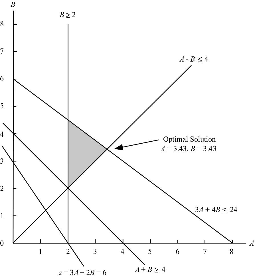
c. S1 = (3.43 + 3.43) - 4 = 2.86
S2 = 24 - [3(3.43) + 4(3.43)] = 0
S3 = 3.43 - 2 = 1.43
S4 = 0 - (3.43 - 3.43) = 0
Constraint2
Constraint1
Constraint3
FeasibleRegion
c. Optimal solution occurs at the intersection of constraints 1 and 2. For constraint 2, B = 10 + A
Substituting for B in constraint 1 we obtain
5A + 5(10 + A) = 400
5A + 50 + 5A = 400 10A = 350 A = 35
B = 10 + A = 10 + 35 = 45
Optimal solution is A = 35, B = 45
d. Because the optimal solution occurs at the intersection of constraints 1 and 2, these are binding constraints.
e. Constraint 3 is the nonbinding constraint. At the optimal solution 1A + 3B = 1(35) + 3(45) = 170. Because 170 exceeds the right-hand side value of 90 by 80 units, there is a surplus of 80 associated with this constraint.
22. a.
b.
Extreme Point Coordinates Profit
1 (0, 0) 5(0) + 4(0) = 0
2 (1700, 0) 5(1700) + 4(0) = 8500
3 (1400, 600) 5(1400) + 4(600) = 9400
4 (800, 1200) 5(800) + 4(1200) = 8800
5 (0, 1680) 5(0) + 4(1680) = 6720
Extreme point 3 generates the highest profit.
c. Optimal solution is A = 1400, C = 600
d. The optimal solution occurs at the intersection of the cutting and dyeing constraint and the inspection and packaging constraint. Therefore these two constraints are the binding constraints.
e. New optimal solution is A = 800, C = 1200
Profit = 4(800) + 5(1200) = 9200
23. a. Let E = number of units of the EZ-Rider produced L = number of units of the Lady-Sport produced
Max 2400E + 1800L s.t.
6E + 3L 2100 Engine time L 280 Lady-Sport maximum 2E + 2.5L 1000 Assembly and testing E,L 0
b.
L Profit = $960,000 Optimal Solution
Frames for Lady-Sport
Assembly and Testing E = 250, L = 200
Number of Lady-Sport Produced
c. The binding constraints are the manufacturing time and the assembly and testing time.
24. a. Let R = number of units of regular model. C = number of units of catcher’s model. Max 5R + 8C
1R + 3/2 C 900 Cutting and sewing 1/2 R + 1/3 C 300 Finishing 1/8 R + 1/4 C 100 Packing and Shipping
c. 5(500) + 8(150) = $3,700
d. C & S 1(500) + 3/2(150) = 725 F 1/2(500) + 1/3(150) = 300 P & S 1/8(500) + 1/4(150) = 100
e.
25. a. Let B = percentage of funds invested in the bond fund S = percentage of funds invested in the stock fund
0.06 B + 0.10 S
B + S = 1
b. Optimal solution: B = 0.3, S = 0.7 Value of optimal solution is 0.088 or 8.8%
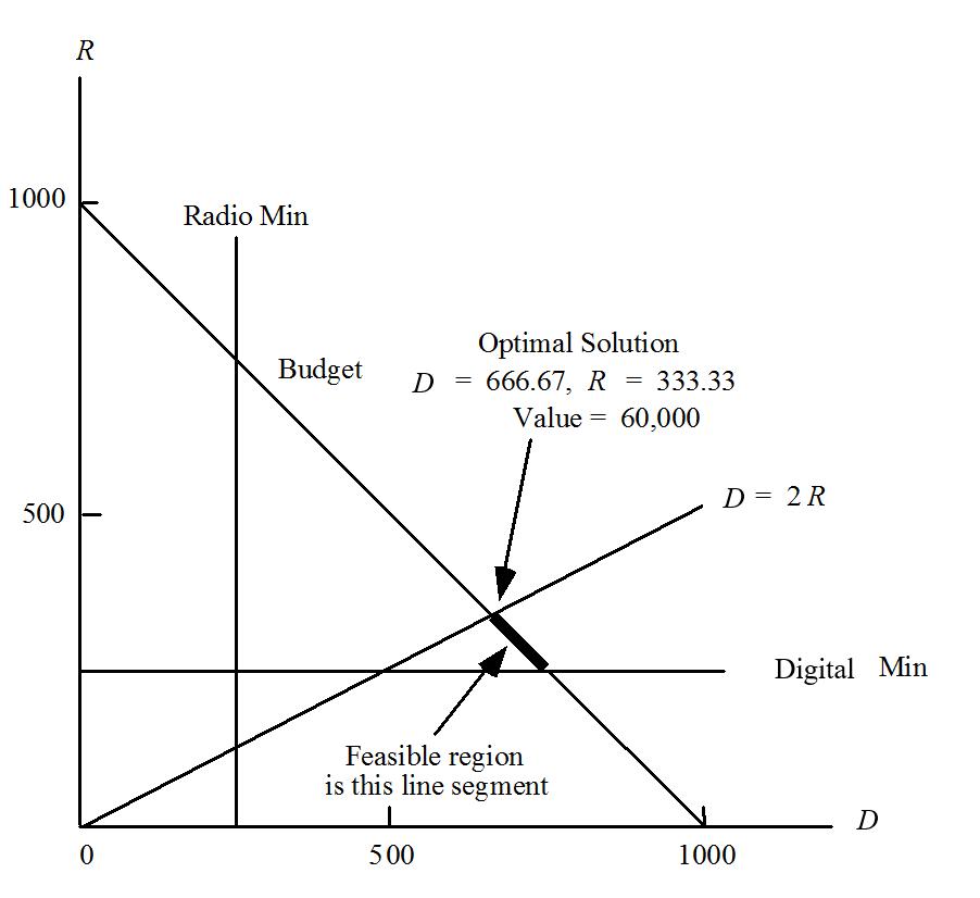
26. a. Let D = amount spent on digital advertising R = amount spent on radio advertising
Max 50D +80R s.t.
D + R = 1000 Budget
D 250 Digital min. R 250 Radio min.
D -2R 0 Digital 2 Radio
27. Let I = Internet fund investment in thousands B = Blue Chip fund investment in thousands
Max 0.12I + 0.09B s.t.
1I + 1B 50 Available investment funds
6I + 4B
Maximum risk for a moderate investor I,B 0
Fund (000s)
b. The third constraint for the aggressive investor becomes 6I + 4B 320
This constraint is redundant; the available funds and the maximum Internet fund investment constraints define the feasible region. The optimal solution is:
The aggressive investor places as much funds as possible in the high return but high risk Internet fund.
c. The third constraint for the conservative investor becomes
6I + 4B 160
This constraint becomes a binding constraint. The optimal solution is
The slack for constraint 1 is $10,000. This indicates that investing all $50,000 in the Blue Chip fund is still too risky for the conservative investor. $40,000 can be invested in the Blue Chip fund. The remaining $10,000 could be invested in low-risk bonds or certificates of deposit.
28. a. Let W = number of jars of Western Foods Salsa produced M = number of jars of Mexico City Salsa produced
Note: units for constraints are ounces
b. Optimal solution: W = 560, M = 240
Value of optimal solution is 860
29. a. Let B = proportion of Buffalo's time used to produce component 1 D = proportion of Dayton's time used to produce component 1
MaximumDailyProduction Component 1 Component 2
Number of units of component 1 produced: 2000B + 600D
Number of units of component 2 produced: 1000(1 - B) + 600(1 - D)
For assembly of the ignition systems, the number of units of component 1 produced must equal the number of units of component 2 produced.
Therefore,
2000B + 600D = 1000(1 - B) + 1400(1 - D)
2000B + 600D = 1000 - 1000B + 1400 - 1400D
3000B + 2000D = 2400
Note: Because every ignition system uses 1 unit of component 1 and 1 unit of component 2, we can maximize the number of electronic ignition systems produced by maximizing the number of units of subassembly 1 produced.
Max 2000B + 600D
In addition, B 1 and D 1.
The linear programming model is: Max 2000B + 600D s.t. 3000B + 2000D = 2400
An Introduction to Linear Programming
The graphical solution is shown below.
Optimal Solution
2000B + 600D = 300
Optimal Solution: B = .8, D = 0
Optimal Production Plan
Buffalo - Component 1 .8(2000) = 1600
Buffalo - Component 2 .2(1000) = 200
Dayton - Component 1 0(600) = 0
Dayton - Component 2 1(1400) = 1400
Total units of electronic ignition system = 1600 per day.
30. a. Let E = number of shares of Eastern Cable C = number of shares of ComSwitch Max 15E + 18C s.t.
c. There are four extreme points: (375,400); (1000,400);(625,1000); (375,1000)
d. Optimal solution is E = 625, C = 1000
return = $27,375
Objective Function Value = 13
Introduction to Linear Programming
(A = 250, B = 100)
(A = 125, B = 225)
(A = 125, B = 350)
Optimal Solution: A = 3, B = 1, value = 5
(1) 3 + 4(1) = 7
(2) 2(3) + 1 = 7
(3) 3(3) + 1.5 = 10.5
= 21 - 7 = 14
= 21 - 10.5 = 10.5 (4) -2(3) +6(1) = 0
= 0 - 0 = 0
Optimal Solution: A = 6, B = 2, value = 34
a.
Feasible Region
Introduction to Linear Programming
(21/4, 9/4) (4,1)
b. There are two extreme points: (A = 4, B = 1) and (A = 21/4, B = 9/4)
c. The optimal solution is A = 4, B = 1
35. a.
Min 6A + 4B + 0S1 + 0S2 + 0S3 s.t.
2A + 1B - S1 = 12 1A + 1B - S2 = 10 1B + S3 = 4
A, B, S1, S2, S3 0
b. The optimal solution is A = 6, B = 4.
c. S1 = 4, S2 = 0, S3 = 0.
36. a. Let T = number of training programs on teaming P = number of training programs on problem solving
Max 10,000T + 8,000P s.t. T 8
Minimum Teaming P 10 Minimum Problem Solving T + P 25 Minimum Total 3 T + 2 P 84 Days Available
T,P 0
Days Available Minimum Problem Solving
Number of Teaming Programs
c. There are four extreme points: (15,10); (21.33,10); (8,30); (8,17)
d. The minimum cost solution is T = 8, P = 17
Total cost = $216,000
37.
Let R = number of containers of Regular Z = number of containers of Zesty
Each container holds 12/16 or 0.75 pounds of cheese
Pounds of mild cheese used = 0.80 (0.75) R + 0.60 (0.75) Z = 0.60 R + 0.45 Z
Pounds of extra sharp cheese used = 0.20 (0.75) R + 0.40 (0.75) Z = 0.15 R + 0.30 Z
Cost of Cheese = Cost of mild + Cost of extra sharp = 1.20 (0.60 R + 0.45 Z) + 1.40 (0.15 R + 0.30 Z) = 0.72 R + 0.54 Z + 0.21 R + 0.42 Z = 0.93 R + 0.96 Z
Packaging Cost = 0.20 R + 0.20 Z
Total Cost = (0.93 R + 0.96 Z) + (0.20 R + 0.20 Z) = 1.13 R + 1.16 Z
Revenue = 1.95 R + 2.20 Z
Profit Contribution = Revenue - Total Cost = (1.95 R + 2.20 Z) - (1.13 R + 1.16 Z) = 0.82 R + 1.04 Z Max 0.82 R + 1.04 Z s.t. 0.60 R + 0.45 Z 8100 Mild 0.15 R + 0.30 Z 3000 Extra Sharp R, Z 0
Optimal Solution: R = 9600, Z = 5200, profit = 0.82(9600) + 1.04(5200) = $13,280
38. a. Let S = yards of the standard grade material per frame P = yards of the professional grade material per frame
Min 7.50S + 9.00P s.t.
0.10S + 0.30P 6 carbon fiber (at least 20% of 30 yards) 0.06S + 0.12P 3 kevlar (no more than 10% of 30 yards)
S + P = 30 total (30 yards)
S, P 0
b.
c.
Extreme Point S = 10 P = 20
Feasible region is the line segment kevlar Extreme Point S = 15 P = 15 carbon fiber
Extreme Point Cost
(15, 15) 7.50(15) + 9.00(15) = 247.50 (10, 20) 7.50(10) + 9.00(20) = 255.00
The optimal solution is S = 15, P = 15
d. Optimal solution does not change: S = 15 and P = 15. However, the value of the optimal solution is reduced to 7.50(15) + 8(15) = $232.50.
e. At $7.40 per yard, the optimal solution is S = 10, P = 20. The value of the optimal solution is reduced to 7.50(10) + 7.40(20) = $223.00. A lower price for the professional grade will not change the S = 10, P = 20 solution because of the requirement for the maximum percentage of kevlar (10%).
39. a. Let S = number of units purchased in the stock fund M = number of units purchased in the money market fund
Optimal Solution: S = 4000, M = 10000, value = 62000
b. Annual income = 5(4000) + 4(10000) = 60,000
c. Invest everything in the stock fund.
40. Let P1 = gallons of product 1 P2 = gallons of product 2
Optimal Solution: P1 = 30, P2 = 25 Cost = $55
41. a. Let R = number of gallons of regular gasoline produced P = number of gallons of premium gasoline produced
Max 0.30R + 0.50P s.t. 0.30
b. Optimal Solution: 40,000 gallons of regular gasoline 10,000 gallons of premium gasoline Total profit contribution = $17,000
Gallons of Regular Gasoline
Introduction to Linear Programming
Satisfies Constraint #2
Infeasibility
Satisfies Constraint #1
Objective Function
Optimal Solution (30/16, 30/16) Value = 60/16
b. New optimal solution is A = 0, B = 3, value = 6.
Unbounded
Feasible Region
= 3
Optimal Solution x2 = 0 x1 = 3, Value = 3
b. Feasible region is unbounded.
c. Optimal Solution: A = 3, B = 0, z = 3.
d. An unbounded feasible region does not imply the problem is unbounded. This will only be the case when it is unbounded in the direction of improvement for the objective function.
46. Let N = number of sq. ft. for national brands G = number of sq. ft. for generic brands
Problem Constraints:

a. Optimal solution is extreme point 2; 180 sq. ft. for the national brand and 20 sq. ft. for the generic brand.
b. Alternative optimal solutions. Any point on the line segment joining extreme point 2 and extreme point 3 is optimal.
c. Optimal solution is extreme point 3; 120 sq. ft. for the national brand and 80 sq. ft. for the generic brand.
optima
Alternative optimal solutions exist at extreme points (A = 125, B = 225) and (A = 250, B = 100).
Cost = 3(125) + 3(225) = 1050 or Cost = 3(250) + 3(100) = 1050
The solution (A = 250, B = 100) uses all available processing time. However, the solution (A = 125, B = 225) uses only 2(125) + 1(225) = 475 hours.
Thus, (A = 125, B = 225) provides 600 - 475 = 125 hours of slack processing time which may be used for other products.
Feasible solutions for constraint requiring 500 gallons of production


Possible Actions:
i. Reduce total production to A = 125, B = 350 on 475 gallons.
ii. Make solution A = 125, B = 375 which would require 2(125) + 1(375) = 625 hours of processing time. This would involve 25 hours of overtime or extra processing time.
iii. Reduce minimum A production to 100, making A = 100, B = 400 the desired solution.
49. a. Let P = number of full-time equivalent pharmacists T = number of full-time equivalent physicians
The model and the optimal solution are shown below:
MIN 40P+10T
S.T.
1) P+T >=250 2) 2P-T>=0
3) P>=90
b.
The optimal solution requires 90 full-time equivalent pharmacists and 160 full-time equivalent technicians. The total cost is $5200 per hour.
The payroll cost using the current levels of 85 pharmacists and 175 technicians is 40(85) + 10(175) = $5150 per hour.
The payroll cost using the optimal solution in part (a) is $5200 per hour.
Thus, the payroll cost will go up by $50
50. Let M = number of Mount Everest Parkas R = number of Rocky Mountain Parkas
100M + 150R s.t.
M + 20R
Note: Students often have difficulty formulating constraints such as the % requirement constraint. We encourage our students to proceed in a systematic step-by-step fashion when formulating these types of constraints. For example:
M must be at least 20% of total production
M 0.2 (total production)
M 0.2 (M + R)
M 0.2M + 0.2R
0.8M - 0.2R 0

Optimal Solution
Profit = $30,000 (65.45,261.82)
The optimal solution is M = 65.45 and R = 261.82; the value of this solution is z = 100(65.45) + 150(261.82) = $45,818. If we think of this situation as an on-going continuous production process, the fractional values simply represent partially completed products. If this is not the case, we can approximate the optimal solution by rounding down; this yields the solution M = 65 and R = 261 with a corresponding profit of $45,650.
51. Let C = number sent to current customers N = number sent to new customers
Note:
Number of current customers that test drive = .25 C
Number of new customers that test drive = .20 N Number sold = .12 ( .25 C ) + .20 (.20 N )
52. Let S = number of standard size rackets O = number of oversize size rackets

53. a. Let R = time allocated to regular customer service N = time allocated to new customer service
1.2R + N s.t.
Optimal solution: R = 50, N = 30, value = 90
HTS should allocate 50 hours to service for regular customers and 30 hours to calling on new customers.
54. a. Let M1= number of hours spent on the M-100 machine M2= number of hours spent on the M-200 machine
Contribution
The optimal decision is to schedule 12.5 hours on the M-100 and 10 hours on the M-200.
55. Mr. Krtick’s solution cannot be optimal. Every department has unused hours, so there are no binding constraints. With unused hours in every department, clearly some more product can be made.
56. No, it is not possible that the problem is now infeasible. Note that the original problem was feasible (it had an optimal solution). Every solution that was feasible is still feasible when we change the constraint to lessthan-or-equal-to, since the new constraint is satisfied at equality (as well as inequality). In summary, we have relaxed the constraint so that the previous solutions are feasible (and possibly more satisfying the constraint as strict inequality).
57. Yes, it is possible that the modified problem is infeasible. To see this, consider a redundant greater-thanor-equal to constraint as shown below. Constraints 2,3, and 4 form the feasible region and constraint 1 is redundant. Change constraint 1 to less-than-or-equal-to and the modified problem is infeasible.
Original Problem:
An Introduction to Linear Programming
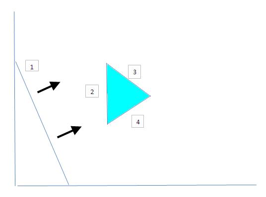
Modified Problem:
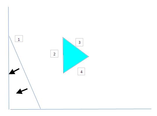
58. It makes no sense to add this constraint. The objective of the problem is to minimize the number of products needed so that everyone’s top three choices are included. There are only two possible outcomes relative to the boss’ new constraint. First, suppose the minimum number of products is <= 15, then there was no need for the new constraint. Second, suppose the minimum number is > 15. Then the new constraint makes the problem infeasible.
Chapter 2
An Introduction to Linear Programming
Case Problem 1: Workload Balancing
1. Production Rate (minutes per printer)
Model Line 1 Line 2 Profit Contribution
3 4 42 DI-950 6 2 87
Capacity: 8 hours 60 minutes/hour = 480 minutes per day
Let D1 = number of units of the DI-910 produced D2 = number of units of the DI-950 produced
The optimal solution is D1 = 0, D2 = 80. The value of the optimal solution is $6960.
Management would not implement this solution because no units of the DI-910 would be produced.
2. Adding the constraint D1 D2 and resolving the linear program results in the optimal solution D1 = 53.333, D2 = 53.333. The value of the optimal solution is $6880.
3. Time spent on Line 1: 3(53.333) + 6(53.333) = 480 minutes
Time spent on Line 2: 4(53.333) + 2(53.333) = 320 minutes
Thus, the solution does not balance the total time spent on Line 1 and the total time spent on Line 2. This might be a concern to management if no other work assignments were available for the employees on Line 2.
4. Let T1 = total time spent on Line 1 T2 = total time spent on Line 2
Whatever the value of T2 is, T1 T2 + 30 T1 T2 - 30
Thus, with T1 = 3D1 + 6D2 and T2 = 4D1 + 2D2
3D1 + 6D2 4D1 + 2D2 + 30
3D1 + 6D2 4D1 + 2D2 30
Hence,
1D1 + 4D2 30
1D1 + 4D2 30
Rewriting the second constraint by multiplying both sides by -1, we obtain
1D1 + 4D2 30
1D1 4D2 30
Adding these two constraints to the linear program formulated in part (2) and resolving we obtain the optimal solution D1 = 96.667, D2 = 31.667. The value of the optimal solution is $6815. Line 1 is scheduled for 480 minutes and Line 2 for 450 minutes. The effect of workload balancing is to reduce the total contribution to profit by $6880 - $6815 = $65 per shift.
5. The optimal solution is D1 = 106.667, D2 = 26.667. The total profit contribution is 42(106.667) + 87(26.667) = $6800
Comparing the solutions to part (4) and part (5), maximizing the number of printers produced (106.667 + 26.667 = 133.33) has increased the production by 133.33 - (96.667 + 31.667) = 5 printers but has reduced profit contribution by $6815 - $6800 = $15. But, this solution results in perfect workload balancing because the total time spent on each line is 480 minutes.
Case Problem 2: Production Strategy
1. Let BP100 = the number of BodyPlus 100 machines produced BP200 = the number of BodyPlus 200 machines produced
s.t.
8
Machining and Welding 5
Painting and Finishing
Assembly, Test, and Packaging
BodyPlus 200 Requirement
BP100, BP200 0
Optimal solution: BP100 = 50, BP200 = 50/3, profit = $26,233.33. Note: If the optimal solution is rounded to BP100 = 50, BP200 = 16.67, the value of the optimal solution will differ from the value shown. The value we show for the optimal solution is the same as the value that will be obtained if the problem is solved using a linear programming software package.
2. In the short run the requirement reduces profits. For instance, if the requirement were reduced to at least 24% of total production, the new optimal solution is BP100 = 1425/28, BP200 = 225/14, with a total profit of $26,290.18; thus, total profits would increase by $56.85. Note: If the optimal solution is rounded to BP100 = 50.89, BP200 = 16.07, the value of the optimal solution will differ from the value shown. The value we show for the optimal solution is the same as the value that will be obtained if the problem is solved using a linear programming software package such as Excel Solver.
3. If management really believes that the BodyPlus 200 can help position BFI as one of the leader's in high-end exercise equipment, the constraint requiring that the number of units of the BodyPlus 200 produced be at least 25% of total production should not be changed. Since the optimal solution uses all of the available machining and welding time, management should try to obtain additional hours of this resource.
Case Problem 3: Hart Venture Capital
1. Let S = fraction of the Security Systems project funded by HVC M = fraction of the Market Analysis project funded by HVC
The solution obtained is shown below:
2.
Thus, the optimal solution is S = 0.609 and M = 0.870. In other words, approximately 61% of the Security Systems project should be funded by HVC and 87% of the Market Analysis project should be funded by HVC.
The net present value of the investment is approximately $2,486,957.
Note: The totals for Year 1 and Year 3 are greater than the amounts available. The reason for this is that rounded values for the decision variables were used to compute the amount required in each year.
3. If up to $900,000 is available in year 1 we obtain a new optimal solution with S = 0.689 and M = 0.820. In other words, approximately 69% of the Security Systems project should be funded by HVC and 82% of the Market Analysis project should be funded by HVC.
The net present value of the investment is approximately $2,550,820. The solution follows:
4. If an additional $100,000 is made available, the allocation plan would change as follows:
5. Having additional funds available in year 1 will increase the total net present value. The value of the objective function increases from $2,486,957 to $2,550,820, a difference of $63,863. But, since the allocation plan shows that $823,400 is required in year 1, only $23,400 of the additional $100,00 is required. We can also determine this by looking at the slack variable for constraint 1 in the new solution. This value, 77049.180, shows that at the optimal solution approximately $77,049 of the $900,000 available is not used. Thus, the amount of funds required in year 1 is $900,000 - $77,049 = $822,951. In other words, only $22,951 of the additional $100,000 is required. The differences between the two values, $23,400 and $22,951, is simply due to the fact that the value of $23,400 was computed using rounded values for the decision variables.

Anderson Sweeney Williams Camm Cochran Fry Ohlmann
An Introduction to Management Science, 15e
Quantitative Approaches to Decision Making
Chapter 2: An Introduction to Linear Programming
2.1 -A Simple Maximization Problem
2.2 -Graphical Solution Procedure
2.3 -Extreme Points and the Optimal Solution
2.4 -Computer Solution of the Par, Inc., Problem
2.5 -A Simple Minimization Problem
2.6 -Special Cases
2.7 -General Linear Programming Notation
Linear Programming (1 of 2)
•Linear programminghas nothing to do with computer programming.
•The use of the word “programming” here means “choosing a course of action.”
•Linear programming involves choosing a course of action when the mathematical model of the problem contains only linear functions.
Linear Programming (2 of 2)
• The maximization or minimization of some quantity is the objective in all linear programming problems.
• All LP problems have constraints that limit the degree to which the objective can be pursued.
• A feasible solution satisfies all the problem's constraints.
• An optimal solution is a feasible solution that results in the largest possible objective function value when maximizing (or smallest when minimizing).
• A graphical solution method can be used to solve a linear program with two variables.
Guidelines for Model Formulation
Problem formulation or modeling is the process of translating a verbal statement of a problem into a mathematical statement.
• Understand the problem thoroughly.
• Describe the objective.
• Describe each constraint.
• Define the decision variables.
• Write the objective in terms of the decision variables.
• Write the constraints in terms of the decision variables.
A Simple Maximization Problem (1
of 4)
Par, Inc., is a small manufacturer of golf equipment and supplies whose management has decided to move into the market for medium-and high-priced golf bags. Par, Inc.’s distributor has agreed to buy all the golf bags Par, Inc., produces over the next three months.
Each golf bag produced will require the following operations:
1. Cutting and dyeing the material
2. Sewing
3. Finishing (inserting umbrella holder, club separators, etc.)
4. Inspection and packaging
This
A Simple Maximization Problem (2 of 4)
A Simple Maximization Problem (3
of 4)
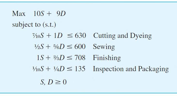
• Par, Inc.’s production is constrained by a limited number of hours available in each department. The director of manufacturing estimates that 630 hours for cutting and dyeing, 600 hours for sewing, 708 hours for finishing, and 135 hours for inspection and packaging will be available for the production of golf bags during the next three months.
• The accounting department analyzed the production data and arrived at prices for both bags that will result in a profit contribution1 of $10 for every standard bag and $9 for every deluxe bag produced.
A Simple Maximization Problem (4 of
The complete model for the Par, Inc., problem is as follows:
Graphical Solution Procedure (1
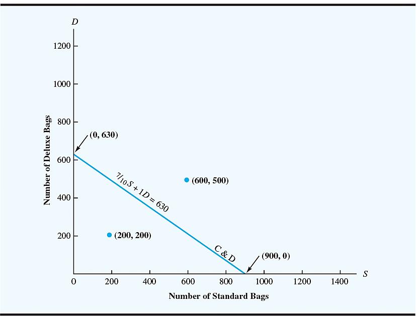
Earlier, we saw that the inequality representing the cutting and dyeing constraint is:
7
10 SD
1630
To show all solution points that satisfy this relationship, we start by graphing the solution points satisfying the constraint as an equality.
Graphical Solution Procedure (2 of 5)
We continue by identifying the solution points satisfying each of the other three constraints.

Graphical Solution Procedure (3 of 5)
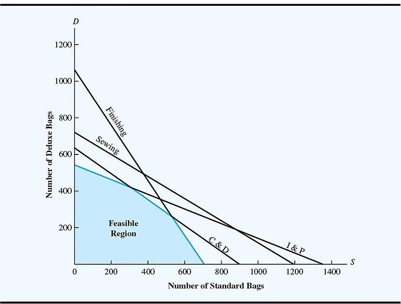
The graph shown identifies the feasible region:
Graphical Solution Procedure (4 of 5)
The optimal solution point is at the intersection of the cutting and dyeing and the finishing constraint lines.
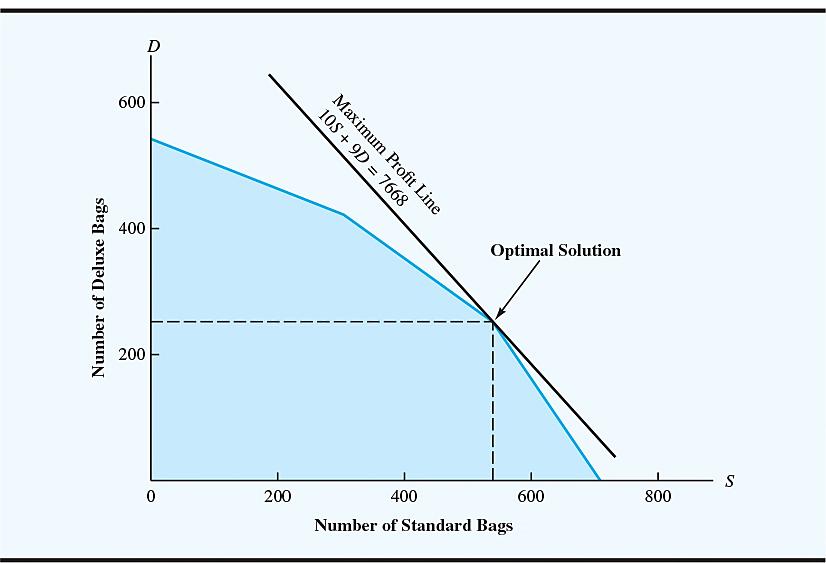
The optimal values of the decision variables S and D must satisfy dyeing and the finishing constraints simultaneously.
This system of equations can be solved using substitution. The exact location of the optimal solution point is S = 540 and D = 252. The optimal production quantities for Par, Inc., are 540 standard bags and 252 deluxe bags, with a resulting profit contribution of 10(540) + 9(252) = $7,668.
Summary of the Graphical Solution Procedure for Maximization Problems
1.Prepare a graph of the feasible solutions for each of the constraints.
2.Determine the feasible region that satisfies all the constraints simultaneously.
3.Draw an objective function line.
4.Move parallel objective function lines toward larger objective function values without entirely leaving the feasible region.
5.Any feasible solution on the objective function line with the largestvalue is an optimal solution.
Slack and Surplus Variables (1 of 2)
• A linear program in which all the variables are nonnegative and all the constraints are equalities is said to be in standard form.
• Standard form is attained by adding slack variables to "less than or equal to" constraints, and by subtracting surplus variables from "greater than or equal to" constraints.
• Slack and surplus variables represent the difference between the left and right sides of the constraints.
• Slack and surplus variables have objective function coefficients equal to 0.
Slack and Surplus Variables (2 of 2)
The complete solution tells management that the production of 540 standard bags and 252 deluxe bags will require all available cutting and dyeing time (630 hours) and all available finishing time (708 hours), while 600 -480 = 120 hours of sewing time and 135 -117 = 18 hours of inspection and packaging time will remain unused. The 120 hours of unused sewing time and 18 hours of unused inspection and packaging time are referred to as slack for the two departments.
Slack Variables (1 of 2)
Often slack variables, are added to the formulation of a linear programming problem to represent the slack, or idle capacity. Unused capacity makes no contribution to profit; thus, slack variables have coefficients of zero in the objective function. After the addition of four slack variables, denoted as , , , and , the mathematical model of the Par, Inc., problem becomes
Slack Variables (2 of 2)
Referring to the standard form of the Par, Inc., problem, we see that at the optimal solution (S = 540 and D = 252), the values for the slack variables are Constraint
On the other hand, the sewing and the inspection and packaging constraints are not binding the feasible region at the optimal solution, which means we can expect some unused time or slack for these two operations.
Extreme Points and the Optimal Solution (1 of 2)
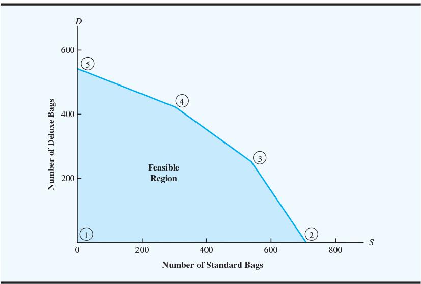
• The corners or vertices of the feasible region are referred to as the extreme points.
• An optimal solution to an LP problem can be found at an extreme point of the feasible region.
• When looking for the optimal solution, you do not have to evaluate all feasible solution points.
• You have to consider only the extreme points of the feasible region.
Extreme Points and the Optimal Solution (2
Here are the 5 extreme points of the feasible region for the Par, Inc., Problem:
Computer Solutions (1 of 3)
• LP problems involving 1000s of variables and 1000s of constraints are now routinely solved with computer packages.
• Linear programming solvers are now part of many spreadsheet packages, such as Microsoft Excel.
• Leading commercial packages include CPLEX, LINGO, MOSEK, Xpress-MP, and Premium Solver for Excel.
Computer Solutions (3 of 3)
1.Prepare a graph of the feasible solutions for each of the constraints.
2.Determine the feasible region that satisfies all the constraints simultaneously.
3.Draw an objective function line.
4.Move parallel objective function lines toward smaller objective function values without entirely leaving the feasible region.
5.Any feasible solution on the objective function line with the smallestvalue is an optimal solution.
A
Simple Minimization Problem (1 of 6)
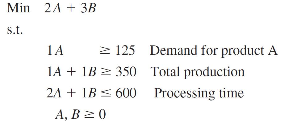
M&D Chemicals produces two products that are sold as raw materials to companies manufacturing bath soaps and laundry detergents.
•M&D’s management specified that the combined production for products A and B must total at least 350 gallons.
•A customer ordered 125 gallons of product A.
•Product A requires 2 hours of processing time per gallon.
•Product B requires 1 hour of processing time per gallon.
•600 hours of processing time are available.
•M&D’s objective is to satisfy these requirements at a minimum total production cost.
•Production costs are $2 per gallon for product A and $3 per gallon for product B.
A Simple Minimization Problem (2
of 6)
After adding the nonnegativity constraints (A, B ≥ 0), we arrive at the following linear program for the M&D Chemicals problem:
A Simple Minimization Problem (3
of 6)
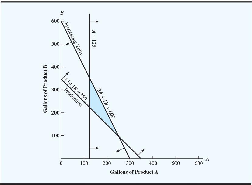
Here is the feasible region for the M&D Chemicals problem:
Note that the objective function 2A + 3B = 800 intersects the feasible region at the extreme point A = 250, B = 100.
A Simple Minimization Problem (4
of 6)
The optimal solution to the M&D Chemicals problem shows that the desired total production of A + B = 350 gallons is achieved by using all processing time: 2A + 1B = 2(250) + 1(100) = 600 hours.
Note that the constraint requiring that product A demand be met has been satisfied with A = 250 gallons. In fact, the production of product A exceeds its minimum level by 250 –125 = 125 gallons. This excess production for product A is referred to as surplus.
A Simple Minimization Problem (5
of 6)
Including two surplus variables, S1 and S2, for the ≥ constraints and one slack variable, S3, for the ≤ constraint, the linear programming model of the M&D Chemicals problem becomes
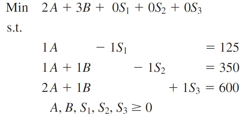
All the constraints are now equalities.
A Simple Minimization Problem (6 of 6)
At the optimal solution of A = 250 and B = 100, the values of the surplus and slack variables are as follows:

Computer Solution
Feasible Region
• The feasible region for a two-variable LP problem can be nonexistent, a single point, a line, a polygon, or an unbounded area.
• Any linear program falls in one of four categories:
• is infeasible
• has a unique optimal solution
• has alternative optimal solutions
• has an objective function that can be increased without bound
• A feasible region may be unbounded and yet there may be optimal solutions. This is common in minimization problems and is possible in maximization problems.
Special Cases (1 of
5)
Alternative Optimal Solutions
In the graphical method, if the objective function line is parallel to a boundary constraint in the direction of optimization, there are alternate optimal solutions, with all points on this line segment being optimal.
Special Cases (2 of 5)
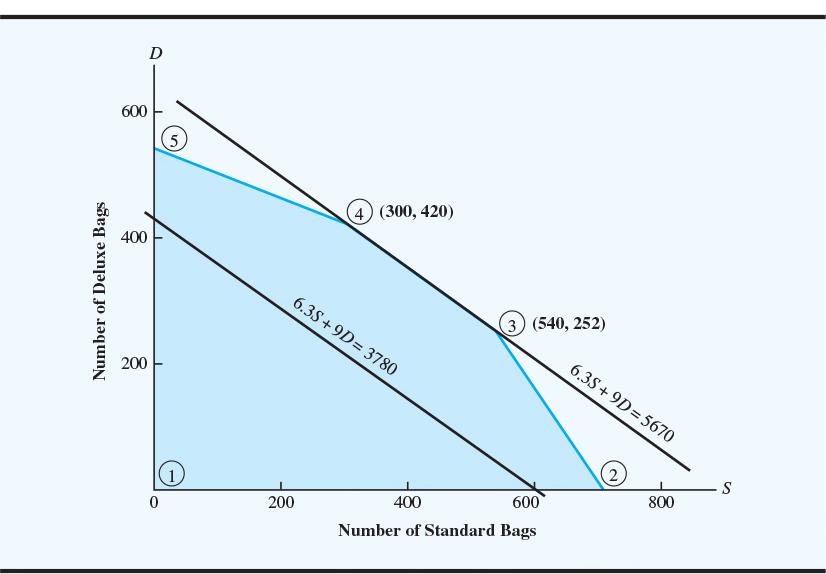
Let’s return to the Par, Inc., problem. However, now assume that the profit for the standard golf bag (S) has decreased to $6.30. The revised objective function becomes 6.3S + 9D.
The objective function values at these two extreme points are identical: 6.3S + 9D = 6.3(300)+9(420) = 5670 and 6.3S + 9D = 6.3(540)+9(252) = 5670
Special Cases (3 of 5)
Furthermore, any point on the line connecting the two optimal extreme points also provides an optimal solution. For example, the solution point (S = 420, D = 336), which is halfway between the two extreme points, also provides the optimal objective function value of 6.3S + 9D = 6.3(420) + 9(336) = 5670.
A linear programming problem with alternative optimal solutions is generally a good situation for the manager or decision maker. It means that several combinations of the decision variables are optimal and that the manager can select the most desirable optimal solution.
Special Cases (4 of 5)
Infeasibility
• No solution to the LP problem satisfies all the constraints, including the non-negativity conditions.
• Graphically, this means a feasible region does not exist.
• Causes include:
•A formulation error has been made.
•Management’s expectations are too high.
•Too many restrictions have been placed on the problem (i.e. the problem is over-constrained).
Special Cases
(5 of 5)
Unbounded
• The solution to a maximization LP problem is unbounded if the value of the solution may be made indefinitely large without violating any of the constraints.
• For real problems, this is the result of improper formulation. (Quite likely, a constraint has been inadvertently omitted.)
General Linear Programming Notation (1 of 3)
We selected decision-variable names of S and D in the Par, Inc., problem and A and B in the M&D Chemicals problem to make it easier to recall what these decision variables represented in the problem. Although this approach works well for linear programs involving a small number of decision variables, it can become difficult when dealing with problems involving a large number of decision variables.
General Linear Programming Notation (2
of 3)
A more general notation that is often used for linear programs uses the letter x with a subscript.
In the Par, Inc., problem, we could have defined the decision variables:
1 x = number of standard bags
2 x = number of deluxe bags
In the M&D Chemicals problem, the same variable names would be used, but their definitions would change:
1 x = number of gallons of product A
2 x = number of gallons of product B
General Linear Programming Notation (3 of 3)
A disadvantage of using general notation for decision variables is that we are no longer able to easily identify what the decision variables actually represent in the mathematical model.
The advantage of general notation is that formulating a mathematical model for a problem that involves a large number of decision variables is much easier.
End of Presentation: Chapter 2

