SSoolluuttiioonnss SSeeccttiioonn 22..11
SSeeccttiioonn 22..11
1. 𝑓 (𝑥) = 2𝑥 2 𝑥 2
a. 𝑎 = 2, 𝑏 = 1, 𝑐 = 2
b. Table of values:
c. 𝑓 (𝑎 + ℎ) = 2(𝑎 + ℎ) 2 (𝑎 + ℎ) 2 = 2(𝑎 2 + 2𝑎ℎ + ℎ 2) (𝑎 + ℎ) 2 = 2𝑎 2 + 4𝑎ℎ + 2ℎ 2 𝑎 ℎ 2
d. 2x^2-x-2
2. 𝑓 (𝑥) = 2𝑥 2 + 𝑥 + 2
a. 𝑎 = 2, 𝑏 = 1, 𝑐 = 2
b. Table of values:
c. 𝑓 (𝑎 + ℎ) = 2(𝑎 + ℎ) 2 + (𝑎 + ℎ) + 2 = 2(𝑎 2 + 2𝑎ℎ + ℎ 2) + (𝑎 + ℎ) + 2 = 2𝑎 2 4𝑎ℎ 2ℎ 2 + 𝑎 + ℎ + 2
d. -2x^2+x+2
3. 𝑓 (𝑥) = 10𝑥 2 5𝑥
a. 𝑎 = 10, 𝑏 = 5, 𝑐 = 0
b. Table of values:
(𝑥)
15
5 30
c. 𝑓 (𝑎 + ℎ) = 10(𝑎 + ℎ) 2 5(𝑎 + ℎ) = 10(𝑎 2 + 2𝑎ℎ + ℎ 2) 5(𝑎 + ℎ) = 10𝑎 2 + 20𝑎ℎ + 10ℎ 2 5𝑎 5ℎ
d. 10x^2-5x
4. 𝑓 (𝑥) = 𝑥 2 50
a. 𝑎 = 1, 𝑏 = 0, 𝑐 = 50
b. Table of values:
3 2 1 0 1 2 3 𝑓 (𝑥) 59 54 51 50 51 54 59
c. 𝑓 (𝑎 + ℎ) = (𝑎 + ℎ) 2 50 = (𝑎 2 + 2𝑎ℎ + ℎ 2) 50 = 𝑎 2 2𝑎ℎ ℎ 2 50 d. -(x^2)-50 (See the margin note next to Quick Example 2 in the text as to the reason for the parentheses.)
5. 𝑓 (𝑥) = 𝑥 2 𝑥 1
a. 𝑎 = 1, 𝑏 = 1, 𝑐 = 1
b. Table of values:
𝑥 3 2 1 0 1 2 3
𝑓 (𝑥) 7 3 1 1 3 7 13
SSoolluuttiioonnss SSeeccttiioonn 22..11
c. 𝑓 (𝑎 + ℎ) = (𝑎 + ℎ) 2 (𝑎 + ℎ) 1 = (𝑎 2 + 2𝑎ℎ + ℎ 2) (𝑎 + ℎ) 1 = 𝑎 2 2𝑎ℎ ℎ 2 𝑎 ℎ 1
d. -(x^2)-x-1 (See margin note next to Quick Example 2 in the textbook as to the reason for the parentheses.)
6. 𝑓 (𝑥) = 3𝑥 2 + 3𝑥 1
a. 𝑎 = 3, 𝑏 = 3, 𝑐 = 1
b. Table of values:
c. 𝑓 (𝑎 + ℎ) = 3(𝑎 + ℎ) 2 + 3(𝑎 + ℎ) 1 = 3(𝑎 2 + 2𝑎ℎ + ℎ 2) + 3(𝑎 + ℎ) 1 = 3𝑎 2 6𝑎ℎ 3ℎ 2 + 3𝑎 + 3ℎ 1
d. -3x^2+3x-1
7. 𝑓 (𝑥) = 𝑥 2 + 3𝑥 + 2 . 𝑎 = 1, 𝑏 = 3, 𝑐 = 2; 𝑏/(2𝑎) = 3/2, 𝑓 ( 3/2) = 1/4 , so: vertex: ( 3/2, 1/4), 𝑦-intercept = 𝑐 = 2 𝑥 2 + 3𝑥 + 2 = (𝑥 + 1)(𝑥 + 2), so: 𝑥-intercepts: 2, 1 𝑎 > 0 so the parabola opens upward.


8. 𝑓 (𝑥) = 𝑥 2 𝑥 . 𝑎 = 1, 𝑏 = 1, 𝑐 = 0; 𝑏/(2𝑎) = 1/2, 𝑓 ( 1/2) = 1/4 , so: vertex: ( 1/2, 1/4), 𝑦-intercept = 𝑐 = 0. 𝑥 2 𝑥 = 𝑥(𝑥 + 1), so: 𝑥-intercepts: 1, 0. 𝑎 < 0 so the parabola opens downward. 9. 𝑓 (𝑥) = 𝑥 2 + 4𝑥 4 . 𝑎 = 1, 𝑏 = 4, 𝑐

𝑥 2 + 2𝑥 + 1 = (𝑥 + 1) 2 , so: 𝑥-intercept: 1 𝑎 > 0 so the parabola opens upward.

11. 𝑓 (𝑥) = 𝑥 2 40𝑥 + 500 𝑎 = 1, 𝑏 = 40, 𝑐 = 500; 𝑏/(2𝑎) = 20, 𝑓 ( 20) = 900 , so: vertex: ( 20, 900), 𝑦-intercept = 𝑐 = 500 𝑥 2 40𝑥 + 500 = (𝑥 + 50)(𝑥 10), so: 𝑥-intercepts: 50, 10 𝑎 < 0 so the parabola opens downward.

12. 𝑓 (𝑥) = 𝑥 2 10𝑥 600 𝑎 = 1, 𝑏 = 10, 𝑐 = 600; 𝑏/(2𝑎) = 5; 𝑓 (5) = 625 , so: vertex: (5, 625), 𝑦-intercept = 𝑐 = 600 𝑥 2 10𝑥 600 = (𝑥 + 20)(𝑥 30), so: 𝑥-intercepts: 20, 30 𝑎 > 0 so the parabola opens upward.

13. 𝑓 (𝑥) = 𝑥 2 + 𝑥 1 𝑎 = 1, 𝑏 = 1, 𝑐 = 1; 𝑏/(2𝑎) = 1/2; 𝑓 ( 1/2) = 5/4 , so: vertex: ( 1/2, 5/4), 𝑦-intercept = 𝑐 = 1. From the quadratic formula: 𝑥-intercepts: 1/2 ± √5/2 . 𝑎 > 0 so the parabola opens upward.

14. 𝑓 (𝑥) = 𝑥 2 + √2𝑥 + 1 𝑎 = 1, 𝑏 = √2 , 𝑐 = 1; 𝑏/(2𝑎) = √2/2 ; 𝑓 ( √2/2) = 1/2 , so: vertex: ( √2/2, 1/2) , 𝑦-intercept = 𝑐 = 1 𝑏 2 4𝑎𝑐 = 2 < 0, so no 𝑥-intercept. 𝑎 > 0 so the parabola opens upward.

15. 𝑓 (𝑥) = 𝑥 2 + 1 . 𝑎 = 1, 𝑏 = 0, 𝑐 = 1; 𝑏/(2𝑎) = 0, 𝑓 (0) = 1 , so: vertex: (0, 1), 𝑦-intercept = 𝑐 = 1.
𝑏 2 4𝑎𝑐 = 4 < 0, so no 𝑥-intercept. 𝑎 > 0 so the parabola opens upward.

16. 𝑓 (𝑥) = 𝑥 2 + 5 . 𝑎 = 1, 𝑏 = 0, 𝑐 = 5; 𝑏/(2𝑎) = 0, 𝑓 (0) = 5 , so vertex: (0, 5), 𝑦-intercept = 𝑐 = 1. From the quadratic formula: 𝑥-intercepts: √5 , √5 . 𝑎 < 0 so the parabola opens downward.

17. 𝑞 = 4𝑝 + 100, 𝑅 = 𝑝𝑞 = 𝑝( 4𝑝 + 100) = 4𝑝 2 + 100𝑝; maximum revenue when 𝑝 = 𝑏/(2𝑎) = $12 50

18. 𝑞 = 3𝑝 + 300, 𝑅 = 𝑝𝑞 = 𝑝( 3𝑝 + 300) = 3𝑝 2 + 300𝑝, maximum revenue when 𝑝 = 𝑏/(2𝑎) = $50

19. 𝑞 = 2𝑝 + 400, 𝑅 = 𝑝𝑞 = 𝑝( 2𝑝 + 400) = 2𝑝 2 + 400𝑝, maximum revenue when 𝑝 = 𝑏/(2𝑎) = $100

20. 𝑞 = 5𝑝 + 1200, 𝑅 = 𝑝𝑞 = 𝑝( 5𝑝 + 1200) = 5𝑝 2 + 1200𝑝, maximum revenue when 𝑝 = 𝑏/(2𝑎) = $120

21. 𝑦 = 0.7955𝑥 2 + 4.4591𝑥 1.6000
22. 𝑦 = 0 7955𝑥 2 4 4591𝑥 1 6000
23. 𝑦 = 1 1667𝑥 2 6 1667𝑥 3 0000
24. 𝑦 = 0 3333𝑥 2 + 1 6667𝑥 + 3 0000
AApppplliiccaattiioonnss
25. a. Positive because the data suggest a curve that is concave up.
b. The data suggest a parabola that is concave up (𝑎 positive) and with 𝑦-intercept around 1, 300. Only choice (C) has both properties.
c. 𝑏/(2𝑎) = 56/8 = 7, which is 1997. Extrapolating in the positive direction leads one to predict more and more
SSoolluuttiioonnss SSeeccttiioonn 22..11 steeply rising military expenditure, which may or may not occur; extrapolating in the negative direction predicts more and more steeply increasing military expenditure as we go back in time, contradicting history. (In fact, military expenditures flattened in the years immediately after 2010.)
26. a. Negative because the data suggest a curve that is concave down.
b. The data suggest a parabola that is concave down (𝑎 negative) and with 𝑦-intercept around 6. Only choice (B) has both properties.
c. 𝑏/(2𝑎) = 0 3/0 08 ≈ 3 75, which is closest to 2004. Extrapolating in either direction leads one to predict eventually negative values for the percentage, which doesn't make sense.
27. The given function 𝐼 (𝑡) = 39𝑡 2 + 800𝑡 3, 000 is quadratic with graph a concave-down parabola (as 𝑎 = 39 is negative). Thus, its vertex is the highest point on the graph and occurs when 𝑡 = 𝑏/(2𝑎) = 800/78 ≈ 10.26, about one quarter of the way into 2010. At that time, imports were about 𝐼 (10 26) = 39(10 26) 2 + 800(10 26) 3, 000 ≈ 1, 100 thousand barrels/day (to two significant digits).
28. The given function 𝑃 (𝑡) = 0.017𝑡 2 0.4𝑡 + 5.23 is quadratic with graph a concave-up parabola (as 𝑎 = 0.017 is positive). Thus, its vertex is the lowest point on the graph and occurs when 𝑡 = 𝑏/(2𝑎) = 0 4/0 034 ≈ 11 76, about three quarters of the way through 2011. At that time, imports were about 𝑃 (11.76) = 0.017(11.76) 2 0.4(11.76) + 5.23 ≈ 2.9 million barrels/day (to two significant digits).
29. The given function 𝑃 (𝑡) = 0 39𝑡 2 + 5 2𝑡 4 1 is quadratic with graph a concave-down parabola (as 𝑎 = 0 39 is negative). Thus, its vertex is the highest point on the graph and occurs when 𝑡 = 𝑏/(2𝑎) = 5.2/0.78 ≈ 6.667, two-thirds way through 2011 At that time, net income was about
𝑃 (𝑡) = 0 39(6 667) 2 + 5 2(6 667) 4 1 ≈ 13 2 billion dollars.
You should not trust this model to continue to be valid long past 2013, as it predicts that General Electric's net income will become negative and continue to decrease without bound. This would soon bankrupt the company.
30. The given function 𝑃 (𝑡) = 1 6𝑡 2 15𝑡 + 46 is quadratic with graph a concave-up parabola (as 𝑎 = 1 6 is positive). Thus, its vertex is the lowest point on the graph and occurs when 𝑡 = 𝑏/(2𝑎) = 15/3 2 ≈ 4 69, around two-thirds way through 2009. At that time, net income was about
𝑃 (𝑡) = 1 6(4 69) 2 15(4 69) + 46 ≈ 10 8 billion dollars.
You should not trust this model to continue to be valid long past 2011, as it predicts that General Electric's net income will increase quicker and quicker. The company's net income would soon become unrealistically large.
31. 𝑞 = 0.5𝑝 + 140. Revenue is 𝑅 = 𝑝𝑞 = 0.5𝑝 2 + 140𝑝. Maximum revenue occurs when 𝑝 = 𝑏/(2𝑎) = $140; the corresponding revenue is 𝑅 = $9, 800
32. 𝑞 = 2𝑝 + 320. Revenue is 𝑅 = 𝑝𝑞 = 2𝑝 2 + 320𝑝. Maximum revenue occurs when 𝑝 = 𝑏/(2𝑎) = $80; the corresponding revenue is 𝑅 = $12, 800.
33. The given data points are (𝑝, 𝑞) = (40, 200, 000) and (60, 160, 000). The line passing through these points is 𝑞 = 2000𝑝 + 280, 000. Revenue is 𝑅 = 𝑝𝑞 = 2000𝑝 2 + 280, 000𝑝. Maximum revenue occurs when 𝑝 = 𝑏/(2𝑎) = 70 houses; the corresponding revenue is 𝑅 = $9, 800, 000.
34. The given data points are (𝑝, 𝑞) = (50, 190, 000) and (70, 170, 000). The line passing through these points is
𝑞 = 1000𝑝 + 240, 000. Revenue is 𝑅 = 𝑝𝑞 = 1000𝑝 2 + 240, 000𝑝. Maximum revenue occurs when 𝑝 = 𝑏/(2𝑎) = 120 houses; the corresponding revenue is 𝑅 = $14, 400, 000.
35. a. A linear demand function has the form 𝑞 = 𝑚𝑝 + 𝑏 (𝑥 is the price 𝑝 and 𝑦 is the demand 𝑞). We are given two points on its graph: (3, 28, 000) and (5, 19, 000). Slope:
𝑚 = 𝑞2 𝑞1 𝑝2 𝑝1 = 19, 000 28, 000 5 3 = 9, 000 2 = 4, 500
Intercept:
𝑏 = 𝑞1 𝑚𝑝1 = 28, 000 ( 4, 500)(3) = 28, 000 + 13, 500 = 41, 500
Thus, the demand equation is 𝑞 = 𝑚𝑝 + 𝑏 = 4, 500𝑝 + 41, 500 b. Revenue:
𝑅 = 𝑝𝑞 = 𝑝( 4, 500𝑝 + 41, 500) = 4, 500𝑝 2 + 41, 500𝑝
For maximum revenue,
𝑝 = 𝑏 2𝑎 = 41, 500 900 ≈ $4 61
The corresponding daily revenue is 𝑅 = 4500(4 61) 2 + 41, 500(4 61) = $95, 680 55
c. The maximum annual revenue the company could have earned was 95, 680 55 × 365≈ $34, 923, 400, which is about $10 million short of what it needed to break even. Therefore, it would not have been possible to break even.
36. a. A linear demand function has the form 𝑞 = 𝑚𝑝 + 𝑏 (𝑥 is the price 𝑝 and 𝑦 is the demand 𝑞). We are given two points on its graph: (5, 14) and (3, 18). Slope:
𝑚 = 𝑞2 𝑞1 𝑝2 𝑝1 = 18 14 3 5 = 4 2 = 2
Intercept:
𝑏 = 𝑞1 𝑚𝑝1 = 14 ( 2)(5) = 24
Thus, the demand equation is 𝑞 = 𝑚𝑝 + 𝑏 = 2𝑝 + 24.
b. Revenue:
𝑅 = 𝑝𝑞 = 𝑝( 2𝑝 + 24) = 2𝑝 2 + 24𝑝
For maximum revenue,
𝑝 = 𝑏 2𝑎 = 24 4 = Ẓ6.
The corresponding daily revenue is 𝑅 = 2(6) 2 + 24(6) = Ẓ72 million.
c. The maximum annual revenue the company could have earned was 72, 000, 000 × 670 = Ẓ48,240,000,000, which is about Ẓ240 million more than it needed to finance the lab. Therefore, it would have been possible to finance the lab.
37. a. The data points are (𝑥, 𝑞) = (2, 280) and (1 5, 560). Thus, 𝑞 = 560𝑥 + 1, 400 and 𝑅 = 𝑥𝑞 = 560𝑥 2 + 1, 400𝑥
b. 𝑃 = 𝑅 𝐶 = 560𝑥 2 + 1400𝑥 30. The largest monthly profit occurs when 𝑥 = 𝑏/(2𝑎) = $1.25 and then 𝑃 = $845 per month.
SSoolluuttiioonnss SSeeccttiioonn 22..11
38. a. The data points are (𝑥, 𝑞) = (8, 400) and (4, 600). Thus, 𝑞 = 50𝑥 + 800 and 𝑅 = 50𝑥 2 + 800𝑥 b. 𝑃 = 𝑅 𝐶 = 50𝑥 2 + 800𝑥 500. The largest weekly profit occurs when 𝑥 = 𝑏/(2𝑎) = $8 per T-shirt and then 𝑃 = $2700 per week.
39. As a function of 𝑞, 𝐶 = 0 5𝑞 + 20. Substituting 𝑞 = 400𝑥 + 1, 200, we get
𝐶 = 0 5( 400𝑥 + 1, 200) + 20 = 200𝑥 + 620
The profit is 𝑃 = 𝑅 𝐶 = 𝑥𝑞 𝐶 = 400𝑥 2 + 1400𝑥 620. The profit is largest when 𝑥 = 𝑏/(2𝑎) = $1.75 per log-on; the corresponding profit is 𝑃 = $605 per month.
40. As a function of 𝑞, 𝐶 = 5𝑞 + 400. Substituting for 𝑞, we get
𝐶 = 5( 40𝑥 + 600) + 400 = 200𝑥 + 3400
The profit is 𝑃 = 𝑅 𝐶 = 𝑥𝑞 𝐶 = 40𝑥 2 + 800𝑥 3400. The profit is largest when 𝑥 = 𝑏/(2𝑎) = $10 per T-shirt; the corresponding profit is 𝑃 = $600 per week.
41. a. The data points are (𝑝, 𝑞) = (10, 300) and (15, 250), so 𝑞 = 10𝑝 + 400
b. 𝑅 = 𝑝𝑞 = 10𝑝 2 + 400𝑝
c. 𝐶 = 3𝑞 + 3000 = 3( 10𝑝 + 400) + 3, 000 = 30𝑝 + 4, 200
d. 𝑃 = 𝑅 𝐶 = 10𝑝 2 + 430𝑝 4, 200. The maximum profit occurs when 𝑝 = 𝑏/(2𝑎) = $21.50.
42. a. The data points are (𝑝, 𝑞) = (2500, 15) and (2000, 20), so 𝑞 = 0 01𝑝 + 40 b. 𝑅 = 50𝑝𝑞 = 50𝑝( 0.01𝑝 + 40) = 0.5𝑝2 + 2000𝑝
c. (i) 𝐶 = 120, 000 + 80, 000𝑞, so (ii) 𝐶 = 120, 000 + 80, 000( 0 01𝑝 + 40) = 800𝑝 + 3, 320, 000
d. 𝑃 = 𝑅 𝐶 = 0 5𝑝 2 + 2800𝑝 3, 320, 000. The maximum profit occurs when 𝑝 = 𝑏/(2𝑎) = $2800 per hour.
43. Here is the Excel tabulation of the data, together with the scatter plot and the quadratic (polynomial order 2) trendline (with the option "Display equation on chart" checked):
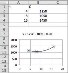
From the trendline, the quadratic model is 𝑓 (𝑡) = 6 25𝑡 2 100𝑡 + 1, 450
To estimate world military expenditure in 2008, substitute the corresponding value 𝑡 = 18, to obtain
𝑓 (18) = 6.25(18) 2 100(18) + 1, 450 = 1, 675 , representing $1,675 billion. The actual figure (from Exercise 25) is $1,600 billion, so the predicted value is $75 billion higher than the actual value.
44. Here is the Excel tabulation of the data, together with the scatter plot and the quadratic (polynomial order 2) trendline (with the option "Display equation on chart" checked):

From the trendline, the quadratic model is
𝑝(𝑡) = 0 05𝑡 2 + 0 5𝑡 + 5 75.
To estimate the percentage of the U.S. Discretionary Budget allocated to education in 2008, substitute the corresponding value 𝑡 = 8, to obtain
𝑝(8) = 0 05(8) 2 + 0 5(8) + 5 75 = 6 55
The actual percentage (from Exercise ??) was 6.3, which is in close agreement with the predicted figure.
45. a. Here is the Excel tabulation of the data, together with a scatter plot and quadratic (polynomial order 2) trendline. The option "Display equation on chart" has been checked.
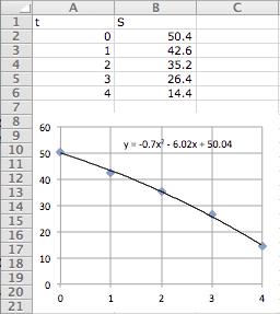
We round the coefficients to two significant digits to get 𝑆(𝑡) = 0.70𝑡 2
b. To predict the sales in 2015 we substitute 𝑡 = 5 and compute
𝑆(5) = 0 70(5) 2 6 0(5) + 50 = 2 5 ≈ 3 million units. Likewise, the 2016 prediction is
+ 50.
SSoolluuttiioonnss SSeeccttiioonn 22..11
𝑆(6) = 0.70(6) 2 6.0(6) + 50 = 11.2 ≈ 11 million units.
Even though we expected 2015 sales to be much lower than the 2014 sales, the 2016 prediction, being negative, shows the danger of extrapolating curve-fitting models.
46. a. Here is the Excel tabulation of the data, together with a scatter plot and quadratic (polynomial order 2) trendline. The option "Display equation on chart" has been checked.
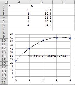
We round the coefficients to two significant digits to get 𝑆(𝑡) = 3 2𝑡 2 + 20𝑡 + 22
b. To predict the sales in 2010 we substitute 𝑡 = 5 and compute
𝑆(5) = 3 2(5) 2 + 20(5) + 22 = 42 million units.
Likewise, the 2011 prediction is
𝑆(6) = 3 2(6) 2 + 20(6) + 22 = 26 8 ≈ 27 million units.
These values are far from the figures of 50.4 and 42.6 million units given in the table in the preceding exercise. This shows the danger of shows the danger of extrapolating curve-fitting models.
CCoommmmuunniiccaattiioonn
aanndd rreeaassoonniinngg eexxeerrcciisseess
47. If 𝑎 = 0, then 𝑓 (𝑥) = 𝑏𝑥 + 𝑐 , a linear function, so its graph is a straight line.
48. Since 𝑐 is the 𝑦-intercept of the graph, 𝑐 = 0 implies that the graph has a 𝑦-intercept of zero, meaning that it passes through the origin.
49. Since the curve is concave up, 𝑎 is positive. Since the 𝑦-intercept is negative, 𝑐 is negative. Hence the correct choice is (C).
50. Since the curve is concave down, 𝑎 is negative. Since the 𝑦-intercept is positive, 𝑐 is positive. Hence the correct choice is (B).
51. Positive; The 𝑥-coordinate of the vertex is negative, so 𝑏/(2𝑎) must be negative. Since 𝑎 is positive (the parabola is concave up), this means that 𝑏 must also be positive to make 𝑏/(2𝑎) negative.
52. Positive; The 𝑥-coordinate of the vertex is positive, so 𝑏/2𝑎 must be positive. Since 𝑎 is negative (the parabola is
SSoolluuttiioonnss SSeeccttiioonn 22..11 concave down), this means that 𝑏 must be positive to make 𝑏/2𝑎 positive.
53. The 𝑥-coordinate of the vertex represents the unit price that leads to the maximum revenue, the 𝑦-coordinate of the vertex gives the maximum possible revenue, the 𝑥-intercepts give the unit prices that result in zero revenue, and the 𝑦 -intercept gives the revenue resulting from zero unit price (which is obviously zero).
54. The 𝑥-coordinate of the vertex gives the time at which the stone reaches its highest point, the 𝑦-coordinate of the vertex gives the maximum height, the 𝑥-intercepts give the times that the stone is at zero height, while the 𝑦-intercept gives the height of the stone at time zero.
55. Graph the data to see whether the points suggest a curve rather than a straight line. If the curve suggested by the graph is concave up or concave down, then a quadratic model would be a likely candidate.
56. Graphing the data shows that neither a linear model nor a quadratic model is appropriate. The curve suggested by the graph is concave down on [0, 4] and concave up on [4, 8]. This is unlike a parabola, which is either always concave up or concave down.
57. No; The graph of a quadratic function is a parabola. In the case of a concave-up parabola, the curve would unrealistically predict sales increasing extremely fast and becoming unrealistically large in the future. In the case of a concave-down parabola, the curve would predict "negative" sales from some point on.
58. Answers may vary. Some uses are: using the model to interpolate; that is, predict missing values inside the domain; using the model for short-term prediction; using a quadratic model to determine maximum possible revenue or profit.
59. If 𝑞 = 𝑚𝑝 + 𝑏 (with 𝑚 < 0), then the revenue is given by 𝑅 = 𝑝𝑞 = 𝑚𝑝 2 + 𝑏𝑝. This is the equation of a parabola with 𝑎 = 𝑚 < 0 and so is concave down. Thus, the vertex is the highest point on the parabola, showing that there is a single highest value for 𝑅, namely, the 𝑦-coordinate of the vertex.
60. The given equation is the equation of a concave-up parabola, and thus has the vertex as its lowest point. The 𝑦 -coordinate of the vertex therefore gives the lowest possible average cost, which occurs when 𝑥 is assigned the value of the 𝑥-coordinate of the vertex.
61. Since 𝑅 = 𝑝𝑞, the demand must be given by 𝑞 = 𝑅 𝑝 = 50𝑝 2 + 60𝑝 𝑝 = 50𝑝 + 60.
62. Since 𝑅 = 𝑝𝑞, the demand is given by 𝑞 = 𝑅 𝑝 = 50𝑝 2 + 60𝑝 + 50 𝑝 = 50𝑝 + 60 + 50 𝑝 . This is not linear.
SSeeccttiioonn 22..22
5. 2*2^x or 2*(2^x)
6. 2*3^x or 2*(3^x)
SSoolluuttiioonnss SSeeccttiioonn 22..22
2^(1-x)
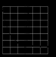

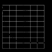

17. 18.

19.
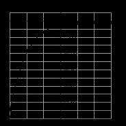
For every increase in 𝑥 by one unit, the value of 𝑓 is multiplied by 3, so 𝑓 is exponential. Since 𝑓 (0) = 4 5 , the exponential model is 𝑓 (𝑥) = 4 5(3 𝑥) For every increase in 𝑥 by one unit, the value of 𝑔 is multiplied by 1/2, so 𝑔 is exponential. Since 𝑔(0) = 2, the exponential model is 𝑔(𝑥) = 2(1/2) 𝑥 , or 2(2 𝑥) 20.
For every increase in 𝑥 by one unit, the value of 𝑓 is multiplied by 2, so 𝑓 is exponential. The values of 𝑔 decrease and then increase, so 𝑔 is not exponential. Since 𝑓 (0) = 2 , the exponential model is 𝑓 (𝑥) = 2(2 𝑥) 21.
When 𝑥 increases from 1 to 0, the value of 𝑓 is multiplied by 1/3, but when 𝑥 is increased from 0 to 1, the value of 𝑓 is multiplied by 3. So 𝑓 is not exponential. When 𝑥 increases from 1 to 0, the value of 𝑔 is multiplied by 3, but when 𝑥 is increased from 1 to 2, the value of 𝑔 is multiplied by 2. So 𝑔 is not exponential.
SSoolluuttiioonnss SSeeccttiioonn 22..22 22.
For every increase in 𝑥 by one unit, the value of 𝑓 is multiplied by 3, so 𝑓 is exponential. Since 𝑓 (0) = 2 7 , the exponential model is 𝑓 (𝑥) = 2 7(3 𝑥) For every increase in 𝑥 by one unit, the value of 𝑔 is multiplied by 0.5, so 𝑔 is exponential. Since 𝑔(0) = 0 75, the exponential model is 𝑔(𝑥) = 0 75(0 5) 𝑥 , or 0 75(2 𝑥)
23.
The values of 𝑓 (𝑥) double for every one-unit increase in 𝑥 except when 𝑥 increases from 1 to 2, when the value of 𝑓 is multiplied by 4/3. Hence 𝑓 is not exponential. On the other hand, 𝑔 is multiplied by 0.2 for every increase by one unit in 𝑥, so 𝑔 is exponential. Since 𝑔(0) = 4, the exponential model is 𝑔(𝑥) = 4(0.2) 𝑥 .
24.
The value of 𝑓 (𝑥) is multiplied by 1/4 when 𝑥 increases from 2 to 1 but halved 𝑥 when increases from 1 to 0. Hence 𝑓 is not exponential. The value of 𝑔(𝑥) is multiplied by 1/2 when 𝑥 increases from 2 to 1 but multiplied by 0.2 when 𝑥 increases from 1 to 2. Hence 𝑔 is not exponential.
25. e^(-2*x) or EXP(-2*x) 26. e^(x/5) or EXP(x/5) 27. 1.01*2.02^(-4*x)
28. 3.42*3^(-x/5)
29. 50*(1+1/3.2)^(2*x)
30. 0.043*(4.5-5/1.2)^(-x)
SSoolluuttiioonnss SSeeccttiioonn 22..22
31. The following solutions also show some common errors you should avoid. 2^(x-1) not 2^x-1
32. 2^(-4*x) not 2^-4*x
33. 2/(1-2^(-4*x)) not 2/1-2^-4*x and not 2/1-2^(-4*x)
34. 2^(3-x)/(1-2^x) or (2^(3-x))/(1-2^x) not 2^3-x/1-2^x and not 2^3-x/(1-2^x)
35. (3+x)^(3*x)/(x+1) or ((3+x)^(3*x))/(x+1)not (3+x)^(3*x)/x+1 and not (3+x^(3*x))/(x+1)
36. 20.3^(3*x)/(1+20.3^(2*x)) or (20.3^(3*x))/(1+20.3^(2*x))not 3^(3*x)/1+20.3^(2*x) and not (20.3^3*x)/(1+20.3^2*x)
37. 2*e^((1+x)/x) or 2*EXP((1+x)/x)not 2*e^1+x/x and not 2*e^(1+x)/x and not 2*EXP(1+x)/x
38. 2*e^(2/x)/x or (2*e^(2/x))/x or 2*EXP(2/x)/x or (2*EXP(2/x))/xnot 2*e^((2/x)/x) and not 2*e^2/x/x and not 2*EXP((2/x)/x)
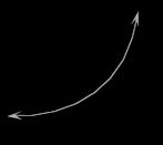
39. In these solutions, 𝑓 1 is black and 𝑓 2 is gray.

41. (Note that the 𝑥-axis shown here crosses at 200, not 0.)

y1 = 300*1.1^x y2 = 300*1.1^(2*x)
43.
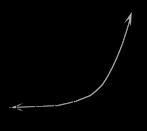
y1 = 2.5^(1.02*x) y2 = e^(1.02*x) or exp(1.02*x)
45. (Note that the 𝑥-axis shown here crosses at 900.)
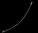
y1 = 1000*1.045^(-3*x) y2 = 1000*1.045^(3*x)
42. (Note that the 𝑥-axis shown here crosses at 95.)
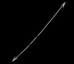
y1 = 100*1.01^(2*x) y2 = 100*1.01^(3*x)
44.

y1 = 2.5^(-1.02*x) y2 = e^(-1.02*x) or exp(-1.02*x)
46. (Note that the 𝑥-axis here crosses at 1,100.)
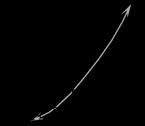
y1 = 1202*1.034^(-3*x) y2 = 1202*1.034^(3*x)
47. Each time 𝑥 increases by 1, 𝑓 (𝑥) is multiplied by 0.5. Also, 𝑓 (0) = 500 So, 𝑓 (𝑥) = 500(0 5) 𝑥
48. Each time 𝑥 increases by 1, 𝑓 (𝑥) is multiplied by 2. Also, 𝑓 (0) = 500 So, 𝑓 (𝑥) = 500(2) 𝑥
49. Each time 𝑥 increases by 1, 𝑓 (𝑥) is multiplied by 3. Also, 𝑓 (0) = 10. So, 𝑓 (𝑥) = 10(3) 𝑥 .
50. Each time 𝑥 increases by 1, 𝑓 (𝑥) is multiplied by 1/3. Also, 𝑓 (0) = 90. So, 𝑓 (𝑥) = 90(1/3) 𝑥 .
51. Each time 𝑥 increases by 1, 𝑓 (𝑥) is multiplied by 225/500 = 0 45 Also, 𝑓 (0) = 500 So, 𝑓 (𝑥) = 500(0 45) 𝑥
52. Each time 𝑥 increases by 1, 𝑓 (𝑥) is multiplied by 3/5 = 0 6 Also, 𝑓 (0) = 5 So, 𝑓 (𝑥) = 5(0 6) 𝑥
SSoolluuttiioonnss SSeeccttiioonn 22..22
53. Write 𝑓 (𝑥) = 𝐴𝑏 𝑥 We have 𝐴𝑏 1 = 110 and 𝐴𝑏 2 = 121 Dividing, 𝑏 = 121/( 110) = 1 1 Substituting, 𝐴(1 1) = 110, so 𝐴 = 100 Thus, 𝑓 (𝑥) = 100(1 1) 𝑥
54. Write 𝑓 (𝑥) = 𝐴𝑏 𝑥 We have 𝐴𝑏 1 = 41 and 𝐴𝑏 2 = 42 025 Dividing, 𝑏 = 42 025/( 41) = 1 025 Substituting, 𝐴(1 025) = 41, so 𝐴 = 41/1 025 = 40 Thus, 𝑓 (𝑥) = 40(1 025) 𝑥
55. We want an equation of the form 𝑦 = 𝐴𝑏 𝑥 Substituting the coordinates of the given points gives 36 = 𝐴𝑏 2
324 = 𝐴𝑏 4
Dividing the second equation by the first gives 324/36 = 9 = 𝑏 2, so 𝑏 = 3. Substituting into the first equation now gives 36 = 𝐴(3) 2 = 9𝐴, so 𝐴 = 36/9 = 4 Hence the model is 𝑦 = 𝐴𝑏 𝑥 = 4(3 𝑥)
56. We want an equation of the form 𝑦 = 𝐴𝑏 𝑥 . Substituting the coordinates of the given points gives
4 = 𝐴𝑏 2
16 = 𝐴𝑏 4
Dividing the second equation by the first gives 16/( 4) = 4 = 𝑏 2, so 𝑏 = 2 Substituting into the first equation now gives 4 = 𝐴(2) 2 = 4𝐴, so 4𝐴 = 14. Hence the model is 𝑦 = 𝐴𝑏 𝑥 = 1(2 𝑥).
57. We want an equation of the form 𝑦 = 𝐴𝑏 𝑥 Substituting the coordinates of the given points gives 25 = 𝐴𝑏 2
0 2 = 𝐴𝑏
Dividing the second equation by the first gives 0 2/( 25) = 0 008 = 𝑏 3, so 𝑏 = 0 2 Substituting into the second equation now gives 0.2 = 0.2𝐴, so 𝐴 = 1. Hence the model is 𝑦 = 𝐴𝑏 𝑥 = 1(0.2 𝑥).
58. We want an equation of the form 𝑦 = 𝐴𝑏 𝑥 Substituting the coordinates of the given points gives
1 2 = 𝐴𝑏
0 108 = 𝐴𝑏 3
Dividing the second equation by the first gives 0 108/1 2 = 0 09 = 𝑏 2, so 𝑏 = 0 3 Substituting into the first equation now gives 1.2 = 0.3𝐴, so 𝐴 = 4. Hence the model is 𝑦 = 𝐴𝑏 𝑥 = 4(0.3 𝑥).
59. Write 𝑓 (𝑥) = 𝐴𝑏 𝑥 We have 𝐴𝑏 1 = 3 and 𝐴𝑏 3 = 6 Dividing, 𝑏 2 = 6/3 = 2, so 𝑏 = √2 ≈ 1 4142 Substituting, 𝐴√2 = 3 , so 𝐴 = 3/√2 ≈ 2 1213 Thus, 𝑦 = 2 1213(1 4142 𝑥)
60. Write 𝑓 (𝑥) = 𝐴𝑏 𝑥 We have 𝐴𝑏 1 = 2 and 𝐴𝑏 4 = 6 Dividing, 𝑏 3 = 6/2 = 3, so 𝑏 = 3 3 √ ≈ 1 4422 Substituting, 𝐴 3 3 √ = 2 , so 𝐴 = 2/ 3 3 √ ≈ 1 3867 Thus, 𝑦 = 1 3867(1 4422 𝑥)
61. Write 𝑓 (𝑥) = 𝐴𝑏 𝑥 We have 𝐴𝑏 2 = 3 and 𝐴𝑏 6 = 2 Dividing, 𝑏 4 = 2/3, so 𝑏 = 2/3 4 √ ≈ 0 9036 Substituting,
𝐴( 2/3 4 √ ) 2 = 3 , so 𝐴 = 3/( 2/3 4 √ ) 2 ≈ 3 6742 Thus, 𝑦 = 3 6742(0 9036 𝑥)
62. Write 𝑓 (𝑥) = 𝐴𝑏 𝑥 We have 𝐴𝑏 1 = 2 and 𝐴𝑏 3 = 1 Dividing, 𝑏 4 = 1/2, so 𝑏 = 1/2 4 √ ≈ 0 8409 Substituting, 𝐴/ 1/2 4 √ = 2 , so 𝐴 = 2 1/2 4 √ ≈ 1 6818 Thus, 𝑦 = 1 6818(0 8409 𝑥)
63. Use the formula 𝑓 (𝑡) = 𝑃 𝑒 𝑟𝑡 with 𝑃 = 5, 000 and 𝑟 = 0 10, giving 𝑓 (𝑡) = 5, 000𝑒 0.10𝑡
64. Use the formula 𝑓 (𝑡) = 𝑃 𝑒 𝑟𝑡 with 𝑃 = 2, 000 and 𝑟 = 0.053, giving 𝑓 (𝑡) = 2, 000𝑒 0.053𝑡 .
65. Use the formula 𝑓 (𝑡) = 𝑃 𝑒 𝑟𝑡 with 𝑃 = 1, 000 and 𝑟 = 0.063, giving 𝑓 (𝑡) = 1, 000𝑒 0 063𝑡 .
66. Use the formula 𝑓 (𝑡) = 𝑃 𝑒 𝑟𝑡 with 𝑃 = 10, 000 and 𝑟 = 0 60, giving 𝑓 (𝑡) = 10, 000𝑒 0 60𝑡
67. 𝑦 = 1.0442(1.7564) 𝑥
68. 𝑦 = 1 0442(0 5694) 𝑥
69. 𝑦 = 15 1735(1 4822) 𝑥
70. 𝑦 = 0.4782(1.8257) 𝑥
AApppplliiccaattiioonnss
71. We want a model of the form 𝑓 (𝑡) = 𝐴𝑏 𝑡 . We are given two points on the graph: (0, 300) and (2, 75). Substituting the coordinates, we get
300 = 𝐴𝑏 0 = 𝐴 Substitute (0, 300).
75 = 𝐴𝑏 2 . Substitute (2, 75).
This gives 𝐴 = 300, 75 = 300𝑏 2, so 𝑏 2 = 75/300 = 0.25, giving 𝑏 = 0.25 1/2 = 0.5, and the model is 𝑓 (𝑡) = 300(0.5) 𝑡 .
After 5 hours, 𝑓 (5) = 300(0 5) 5 = 9 375 mg.
72. We want a model of the form 𝑓 (𝑡) = 𝐴𝑏 𝑡 . We are given two points on the graph: (0, 200) and (2, 112.5). Substituting the coordinates, we get
200 = 𝐴𝑏 0 = 𝐴 Substitute (0, 200).
112 5 = 𝐴𝑏 2 . Substitute (2, 112.5).
This gives 𝐴 = 200, 112 5 = 200𝑏 2 , so 𝑏 2 = 112 5/200 = 0 5625, giving 𝑏 = 0 5625 1/2 = 0 75, and the model is 𝑓 (𝑡) = 200(0.75) 𝑡 .
After 4 hours, 𝑓 (4) = 200(0 75) 4 ≈ 63 mg/dL.
73. a. Linear model: 𝐹 = 𝑚𝑡 + 𝑏
Points: (4, 200) and (10, 590)
Slope: 𝑚 = 𝐹 2 𝐹 1 𝑡2 𝑡1 = 590 200 10 4 = 65
SSoolluuttiioonnss SSeeccttiioonn 22..22
Intercept: 𝑏 = 𝐹 1 𝑚𝑡1 = 200 (65)(4) = 60
Model: 𝐹 = 𝑚𝑡 + 𝑏 = 65𝑡 60
Exponential model: 𝐹 = 𝐴𝑏 𝑡
Substitute (4, 200): 200 = 𝐴𝑏 4; substitute (10, 590): 590 = 𝐴𝑏 10. Now divide the second equation by the first:
590
200 = 𝑏 10 𝑏 4 = 𝑏 6
2.95 = 𝑏 6
𝑏 = (2 95) 1/6 ≈ 1 19758 ≈ 1 20
Substituting the value of 𝑏 in the first equation now gives
200 ≈ 𝐴(1 19758) 4 ≈ 2 0569𝐴, so
𝐴 ≈ 200 2.0569 ≈ 97 2
Model: 𝐹 = 𝐴𝑏 𝑡 = 97 2(1 20) 𝑡
The exponential model is applicable: The successive ratios of the values of 𝐹 are not too far from 𝑏 2 ≈ 1 44 The successive differences climb steadily, making a linear model not appropriate.
b. The year 2008 corresponds to 𝑡 = 8, and so 𝐹 = 𝐴𝑏 𝑡 = 97 2(1 20) 8 ≈ 418 tons, not too far from the projected figure.
74. a. Linear model: 𝐼 = 𝑚𝑡 + 𝑏
Points: (6, 10.7) and (10, 34.2)
Slope: 𝑚 = 𝐼 2 𝐼 1 𝑡2 𝑡1 = 34 2 10 7 10 6 = 5.875 ≈ 5.88
Intercept: 𝑏 = 𝐼 1 𝑚𝑡1 = 10 7 (5 875)(6) = 24 55 ≈ 24 6
Model: 𝐼 = 5 88𝑡 24 6
Exponential model: 𝐼 = 𝐴𝑏 𝑡
Substitute (6, 10 7): 10 7 = 𝐴𝑏 6; substitute (10, 34 2): 34 2 = 𝐴𝑏 10. Now divide the second equation by the first: 34.2 10.7 = 𝑏 10 𝑏 6 = 𝑏 4 3.196 = 𝑏 4 𝑏 = (3.196) 1/4 ≈ 1.33706 ≈ 1.34.
Substituting the value of 𝑏 in the first equation now gives 10.7 ≈ 𝐴(1.33706) 6 ≈ 5.714𝐴, so 𝐴 ≈ 10.7 5.714 ≈ 1 87
Model: 𝐼 = 1 87(1 34) 𝑡
The exponential model is applicable: The successive ratios of the values of 𝐼 are not too far from 𝑏. The successive differences climb steadily, making a linear model not appropriate.
SSoolluuttiioonnss SSeeccttiioonn 22..22
b. The year 2008 corresponds to 𝑡 = 8, and so 𝐼 = 𝐴𝑏 𝑡 = 1.87(1.34) 8 ≈ $19.4 billion, not too far from the actual figure.
75. a. Let 𝑃 = 𝐴𝑏 𝑡 million people. We are given the data points (0, 180) and (50, 309). Substituting them into the equation 𝑃 = 𝐴𝑏 𝑡 gives 𝐴 = 180
309 = 180𝑏 50 so 𝑏 50 = 309/180, which gives 𝑏 = (309/180) 1/50 ≈ 1 01087 Thus, the model is 𝑃 (𝑡) = 180(1 01087) 𝑡 million people.
b. Rounding to 4 significant digits gives 180(1 011) 𝑡 Substituting 𝑡 = 50 gives 𝑃 (50) = 180(1 011) 50 ≈ 311 ≠ 309
Rounding to 5 significant digits gives 180(1.0109) 𝑡 . Substituting 𝑡 = 50 gives 𝑃 (50) = 180(1.0109) 50 ≈ 310 ≠ 309. Rounding to 6 significant digits gives 180(1.01087) 𝑡 . Substituting 𝑡 = 50 gives 𝑃 (50) = 180(1.01087) 50 ≈ 309, which is accurate to 3 significant digits. Therefore, we should round to at least 6 significant digits. (But the values are still accurate to only 3 significant digits.)
c. When 𝑡 = 60, 𝑃 = 180(1 01087) 60 ≈ 344 million people.
76. a. Let 𝑃 = 𝐴𝑏 𝑡 billion people. We are given the data points (0, 2 56) and (61, 6 91). Substituting them into the equation 𝑃 = 𝐴𝑏 𝑡 gives 𝐴 = 2.56
6.91 = 2 56𝑏 61
so 𝑏 61 = 6.91/2.56, which gives 𝑏 = (6.91/2.56) 1/61 ≈ 1.01641. Thus, the model is 𝑃 (𝑡) = 2.56(1.01641) 𝑡 billion people.
b. Rounding to 4 significant digits gives 2.56(1 016) 𝑡 Substituting 𝑡 = 61 gives 𝑃 (61) = 2 56(1 016) 61 ≈ 6 74 ≠ 6 91 Rounding to 5 significant digits gives 2.56(1 0164) 𝑡 Substituting 𝑡 = 61 gives 𝑃 (61) = 2 56(1 0164) 61 ≈ 6 91, which is accurate to 3 significant digits. Therefore, we should round to at least 5 significant digits. (But the values are still accurate to only 3 significant digits.)
c. When 𝑡 = 950, 𝑃 = 2.56(1.01641) 950 ≈ 0.000000493 billion ≈ 493 people. Since this is absurd, it follows that the exponential model does not apply over the long term.
77. a. Let 𝑦 be the number of frogs in year 𝑡, with 𝑡 = 0 representing 2 years ago; we seek a model of the form 𝑦 = 𝐴𝑏 𝑡 We are given the initial value of 𝐴 = 50, 000 and are told that 50, 000𝑏 2 = 75, 000 This gives 𝑏 = (75, 000/50, 000) 1/2 = 1 5 1/2 Thus, 𝑦 = 50, 000(1 5 1/2) 𝑡 = 50, 000(1 5 𝑡/2)
b. When 𝑡 = 3, 𝑦 = 50, 000(1.5) 3/2 = 91, 856 tags.
78. a. Let 𝑦 be the number of flies in year 𝑡, with 𝑡 = 0 representing 3 years ago; we seek a model of the form 𝑦 = 𝐴𝑏 𝑡
We are given the initial value of 𝐴 = 4, 000 and we are told that 4, 000𝑏 3 = 7, 000 This gives 𝑏 = (7, 000/4, 000) 1/3 = 1 75 1/3 Thus, 𝑦 = 4, 000(1 75 1/3) 𝑡 = 4, 000(1 75 𝑡/3)
b. When 𝑡 = 4, 𝑦 = 4, 000(1 75 4/3) = 8, 435 flies.
79. If 𝑦 represents the size of the culture at time 𝑡, then 𝑦 = 𝐴𝑏 𝑡 We are told that the initial size is 1,000, so 𝐴 = 1, 000. We are told that the size doubles every 3 hours, so 𝑏 3 = 2, or 𝑏 = 2 1/3 . Thus,
𝑦 = 1, 000(2 1/3) 𝑡 = 1, 000(2 𝑡/3). There will be 1, 000(2 48/3) = 65, 536, 000 bacteria after 2 days.
80. If 𝑦 represents the size of the culture at time 𝑡, then 𝑦 = 𝐴𝑏 𝑡 We are told that the initial size is 1,000, so
𝐴 = 1, 000 We are told that 𝑦 = 1, 500 when 𝑡 = 2, so 1, 500 = 1, 000𝑏 2 , giving 𝑏 = 1 5 1/2 Thus, 𝑦 = 1, 000(1 5 1/2) 𝑡 = 1, 000(1 5 𝑡/2) There will be 1, 000(1 5 48/2) ≈ 16, 800, 000 bacteria after 2 days.
81. The desired model is 𝐴(𝑡) = 𝐴𝑏 𝑡. At time 𝑡 = 0 (March 17, 2003) the number of cases was 167, so 𝐴 = 167. Since the number was increasing by 18% each day, the number of cases is multiplied by 1.18 each day, so 𝑏 = 1.18. Hence, the model is 𝐴(𝑡) = 167(1 18) 𝑡. Since March 31, 2003 corresponds to 𝑡 = 14, the number of cases was about
𝐴(14) = 167(1 18) 14 ≈ 1, 695
82. The desired model is 𝐴(𝑡) = 𝐴𝑏 𝑡. At time 𝑡 = 0 (April 1, 2003) the number of cases was 1,804, so 𝐴 = 1, 804 Since the number was increasing by 4% each day, the number of cases is multiplied by 1.04 each day, so 𝑏 = 1.04. Hence, the model is 𝐴(𝑡) = 1, 804(1 04) 𝑡. Since April 30, 2003 corresponds to 𝑡 = 29, the number of cases was about 𝐴(14) = 1, 804(1 04) 29 ≈ 5, 626
83. The desired model is 𝐶(𝑡) = 𝐴𝑒 𝑟𝑡. At time 𝑡 = 0 (April 1, 2014) the number of cases was 100, so 𝐴 = 100 Since the number was increasing at a continuous rate of 72% per month, 𝑟 = 0.72. Hence, the model is 𝐶(𝑡) = 100𝑒 0.72𝑡 . Since August 1, 2014 corresponds to 𝑡 = 4, the number of cases was about 𝐶(4) = 100𝑒 0 72 × 4 ≈ 1, 781
84. The desired model is 𝐷(𝑡) = 𝐴𝑒 𝑟𝑡. At time 𝑡 = 0 (April 1, 2014) the number of deaths was 90, so 𝐴 = 90 Since the number was increasing at a continuous rate of 60% per month, 𝑟 = 0 60. Hence, the model is 𝐷(𝑡) = 90𝑒 0.60𝑡 Since October 1, 2014 corresponds to 𝑡 = 6, the number of deaths was about 𝐷(6) = 90𝑒 0 60 × 6 ≈ 3, 294.
85. Apply the formula
𝐴(𝑡) = 𝑃 (1 + 𝑟 𝑚 ) 𝑚𝑡
with 𝑃 = 5, 000, 𝑟 = 0 05/100 = 0 0005, and 𝑚 = 12 We get the model
𝐴(𝑡) = 5, 000(1 + 0 0005/12) 12𝑡
In August 2020 (𝑡 = 7), the deposit would be worth 5, 000(1 + 0.0005/12) 12(7) ≈ $5, 018.
86. Apply the formula
𝐴(𝑡) = 𝑃 (1 + 𝑟 𝑚 ) 𝑚𝑡 with 𝑃 = 4, 000, 𝑟 = 0.0061, and 𝑚 = 365. We get the model
𝐴(𝑡) = 4, 000(1 + 0.0061/365) 365𝑡
In August 2021 (𝑡 = 8), the deposit would be worth 4, 000(1 + 0.0061/365) 365(8) ≈ $4, 200.
87. From the answer to Exercise 85, the value of the investment after 𝑡 years is
𝐴(𝑡) = 5, 000(1 + 0.0005/12) 12𝑡 .
TI-83/84 Plus: Enter Y1 = 5000*(1+0.0005/12)^(12*X), Press [2nd] [TBLSET], and set Indpnt to Ask. (You do this once
SSoolluuttiioonnss SSeeccttiioonn 22..22 and for all; it will permit you to specify values for 𝑥 in the table screen.) Then, press [2nd] [TABLE], and you will be able to evaluate the function at several values of 𝑥. Here are some values of 𝑥 and the resulting values of Y1.
𝑥 18 19 20 21
Y1 5045.20 5047.73 5050.25 5052.78
Notice that Y1 first exceeds 5,050 when 𝑥 = 20 Since 𝑥 = 0 represents August 2013, 𝑥 = 20 represents August 2033, so the investment will first exceed $5,050 in August 2033.
88. From the answer to Exercise 86, the value of the investment after 𝑡 years is
𝐴(𝑡) = 4, 000(1 + 0 0061/365) 365𝑡
TI-83/84 Plus: Enter Y1 = 4000*(1+0.0061/365)^(365*X), Press [2nd] [TBLSET], and set Indpnt to Ask. (You do this once and for all; it will permit you to specify values for 𝑥 in the table screen.) Then, press [2nd] [TABLE], and you will be able to evaluate the function at several values of 𝑥. Here are some values of 𝑥 and the resulting values of Y1.
𝑥 14 15 16 17
Y1 4356.61 4383.26 4410.08 4437.07
Notice that Y1 first exceeds 4,400 when 𝑥 = 16. Since 𝑥 = 0 represents August 2013, 𝑥 = 16 represents August 2029, so the investment will first exceed $4,400 in August 2029.
89. From the continuous compounding formula, 1, 000𝑒 0.04 × 10 = $1, 491 82, of which $491.82 is interest.
90. From the continuous compounding formula, 2, 000𝑒 0 31 × 10 = $44, 395.90, of which $42,395.90 is interest.
91. We use the continuous compounding formula 𝐴 = 𝑃 𝑒 𝑟𝑡. We are told 𝑟 = 0.089. At time 𝑡 = 0 (2011), sales were 4.3 million, so 𝐴 = 4 3. Hence, the model is
𝐴(𝑡) = 4 3𝑒 0.089𝑡 million homes.
In 2012, 𝑡 = 1, so
𝐴(1) = 4 3𝑒 0 089(1) ≈ 4 7 million homes.
In 2014, 𝑡 = 3, so
𝐴(3) = 4.3𝑒 0 089(3) ≈ 5.6 million homes.
92. We use the continuous compounding formula 𝐴 = 𝑃 𝑒 𝑟𝑡. We are told 𝑟 = 0.085. At time 𝑡 = 0 (2011), prices were $166 thousand, so 𝐴 = 166. Hence, the model is
𝐴(𝑡) = 166𝑒 0.085𝑡 thousand dollars.
In 2013, 𝑡 = 2, so
𝐴(2) = 166𝑒 0 085(2) ≈ $197 thousand.
In 2015, 𝑡 = 4, so
𝐴(4) = 166𝑒 0 085(4) ≈ $233 thousand.
93. a. The years 1950, 2000, 2050, and 2100 correspond to 𝑡 = 200, 250, 300, and 350 respectively. Technology formula: 280*e^(0.00127x)
year 1950 2000 2050 2100
𝑡 200 250 300 350
b. Testing decades between 2000 (𝑡 = 250) and 2050, we find that 𝐶(280) ≈ 399.6 and 𝐶(290) ≈ 404.7. Testing individual years between 𝑡 = 280 and 𝑡 = 290, we find that the level surpasses 400 for the first time when 𝑡 = 281
Thus, to the nearest decade, the level passes 400 in 2030 (𝑡 = 280).
94. a. The years 1950, 2000, 2050, and 2100 correspond to 𝑡 = 200, 250, 300, and 350 respectively. Technology formula: 720*e^(0.00351x)
𝐶(𝑡) parts per million 361 385 410 437 year 1950 2000 2050 2100
𝑡 200 250 300 350
𝐶(𝑡) parts per billion 1,450 1,730 2,060 2,460
b. Testing decades between 2000 (𝑡 = 250) and 2050, we find that 𝐶(290) ≈ 1, 990 and 𝐶(300) ≈ 2, 060 Testing individual years between 𝑡 = 290 and 𝑡 = 300, we find that the level surpasses 2,000 for the first time when 𝑡 = 292
Thus, to the nearest decade, the level passes 2,000 in 2040 (𝑡 = 290).
95. a. Here is the Excel tabulation of the data, together with the scatter plot and the exponential trendline (with the option "Display equation on chart" checked):

Note that the displayed model has the form 𝑃 (𝑡) = 0.3394𝑒 0.1563𝑡. To express this in the form 𝐴(𝑏) 𝑡 we write 0.339𝑒 0.1563𝑡 = 0.339(𝑒 0.1563) 𝑡 ≈ 0.339(1.169) 𝑡 so the model is
𝑃 (𝑡) = 0 339(1 169) 𝑡
b. In 2005, 𝑡 = 11, so the predicted cost is
𝑃 (15 = 0 339(1 169) 11
≈ $1 9 million.
96. a. Here is the Excel tabulation of the data, together with the scatter plot and the exponential trendline (with the option "Display equation on chart" checked):
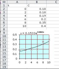
Note that the displayed model has the form 𝑃 (𝑡) = 0.1533𝑒 0.0863𝑡 . To express this in the form 𝐴(𝑏) 𝑡 we write
0 153𝑒 0.0863𝑡 = 0 153(𝑒 0.1563) 𝑡 ≈ 0 153(1 090) 𝑡 so the model is
𝑃 (𝑡) = 0 153(1 090) 𝑡
b. In 2005, 𝑡 = 15, so the predicted cost is
𝑃 (15) = 0 153(1 090) 15
≈ $0 56 million.
97. a. Here is the Excel tabulation of the data, together with the scatter plot and the exponential trendline (with the option "Display equation on chart" checked):
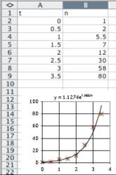
Note that the displayed model has the form 𝑛(𝑡) = 1.1274𝑒 1.2652𝑡 . To express this in the form 𝐴(𝑏) 𝑡 we write 1.1274𝑒 1.2652𝑡 = 1.1274(𝑒 1.2652) 𝑡 ≈ 1.1274(3.5438) 𝑡 which rounds to 1.127(3.544) 𝑡 and so the model is
𝑛(𝑡) = 1 127(3 544) 𝑡
b. 𝑏 = 3.544, so Facebook membership each year was 3.544 times that of the year before.
c. At the start of 2009, 𝑡 = 4, so the predicted membership is
𝑛(4) = 1.127(3.544) 4 ≈ 178 million members.
98. a. Here is the Excel tabulation of the data, together with the scatter plot and the exponential trendline (with the option "Display equation on chart" checked):
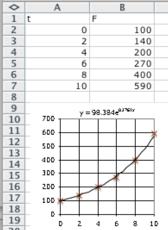
Note that the displayed model has the form 𝐹 (𝑡) = 98 384𝑒 0.1761𝑡 To express this in the form 𝐴(𝑏) 𝑡 we write
98 384𝑒 0.1761𝑡 = 98 384(𝑒 0.1761) 𝑡 ≈ 98 384(1 193) 𝑡 and so the model is
𝐹 (𝑡) = 98 384(1 193) 𝑡
b. 𝑏 = 1 193, so Freon production each year was 1.193 times that of the year before.
c. In 2009, 𝑡 = 9, so the predicted production is
𝐹 (9) = 98.384(1.193) 9 ≈ 482 tons.
CCoommmmuunniiccaattiioonn
aanndd rreeaassoonniinngg eexxeerrcciisseess
99. (B) An exponential function eventually becomes larger than any polynomial.
100. (B) An exponential decay function eventually becomes smaller than the reciprocal of any polynomial (see Exercise 99).
101. Exponential functions of the form 𝑓 (𝑥) = 𝐴𝑏 𝑥 (𝑏 > 1) increase rapidly for large values of 𝑥. In real-life situations, such as population growth, this model is reliable only for relatively short periods of growth. Eventually, population growth tapers off because of pressures such as limited resources and overcrowding.
102. If an investment earns 5% compounded continuously, it is as if interest is being added every moment. Thus, the interest for 1 month will have been calculated on a growing amount, rather than on the original fixed (smaller) amount used for interest compounded monthly.
103. The article was published about a year before the "housing bubble" burst in 2006, whereupon, contrary to the prediction of the graph, house prices started to fall and continued to drop for several years. This shows the danger of using any mathematical model to extrapolate. However, the blogger was cautious in the choice of words, claiming only to be estimating what the future U.S. median house price "might be."
104. Suppose for the sake of argument that the model had been constructed around 𝑡 = 20 (1993). Then the resulting exponential model would have predicted house prices reasonably accurately for around 12 more years. It is just coincidence that the particular model was created a year before prices started to fall. In general, exponential models are very good at extrapolating current trends; it is only when things go awry that they become unreliable.
105. Linear functions are better for cost models where there is a fixed cost and a variable cost and for simple interest, where interest is paid only on the original amount invested. Exponential models are better for compound interest and population growth. In both of these latter examples, the rate of growth depends on the current number of items, rather than on a fixed initial quantity.
SSoolluuttiioonnss SSeeccttiioonn 22..22
106. Quadratic models are better for revenue and profit functions where demand depends linearly on the price. Exponential models are better for compound interest and population growth.
107. Take the ratios 𝑦2 /𝑦1 and 𝑦3 /𝑦2 If they are the same, the points fit on an exponential curve.
108. For the points to fit on an exponential curve we must have 𝑦2 /𝑦1 = 𝑦3 /𝑦2 , hence 𝑦3 = 𝑦2 2/𝑦1
109. This reasoning is suspect. The bank need not use its computer resources to update all the accounts every minute but can instead use the continuous compounding formula to calculate the balance in any account at any time as needed.
110. This banker is correct. In fact, offering continuous compounding at a rate of 𝑟 is the same thing as offering daily compounding at an ever so slightly higher rate. The only difference may be the bank's policy on giving interest for a portion of a day.
SSoolluuttiioonnss SSeeccttiioonn 22..33
SSeeccttiioonn 22..33
1. log4 𝑦
2. 6 𝑦
3. 8. Note that 𝑏 log𝑏 𝑎 = 𝑎 for any 𝑎 and 𝑏, since log𝑏 𝑎 is the power to which you raise 𝑏 to get 𝑎
4. 𝑥. This is a special case of the reasoning in ??
5. 𝑥. To what power to you raise 𝑒 to get 𝑒 𝑥? 𝑥!
6. ln√𝑎 = ln 𝑎 1/2 = 1 2 ln 𝑎
7. 𝑓 (𝑥) = log4 𝑥 . We plot some points and draw the graph: 8. 𝑓 (𝑥) = log5 𝑥 . We plot some points and draw the graph:
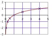
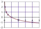
9. 𝑓 (𝑥) = log1/4 𝑥 . We plot some points and draw the graph:
(𝑥) 2 1 1/2 0 1/2 1
(𝑥) 2 1 0 1

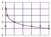
10. 𝑓 (𝑥) = log1/5 𝑥 . We plot some points and draw the graph:
(𝑥) 2 1 0 1
11. 𝑓 (𝑥) = log4 𝑥 + 1 . We plot some points and draw the graph:
𝑥 1/16 1/4 1/2 1 2 4
12. 𝑓 (𝑥) = log5 𝑥 1 . We plot some points and draw the graph:
𝑓 (𝑥) 1 0 1/2 1 3/2 2 𝑥 1/25 1/5 1 5 𝑓 (𝑥) 3 2 1 0

13. 𝑓 (𝑥) = log4 (𝑥 1) . We plot some points and draw the graph:
𝑥 17/16 5/4 3/2 2 3 5
𝑓 (𝑥) 2 1 1/2 0 1/2 1


14. 𝑓 (𝑥) = log5 (𝑥 + 1) . We plot some points and draw the graph:
𝑥 24/25 4/5 0 4
𝑓 (𝑥) 2 1 0 1

15. 𝑄 = 1, 000 when 𝑡 = 0; half-life = 1. We want a model of the form 𝑄 = 𝑄0 𝑒 𝑘𝑡 for suitable 𝑄0 and 𝑘. We are given 𝑄0 = 1, 000. For 𝑘, we use the formula 𝑡ℎ 𝑘 = ln 2 with 𝑡ℎ = half-life = 1, so 𝑘 = ln 2, and the model is 𝑄 = 𝑄0 𝑒 𝑘𝑡 = 1, 000𝑒 𝑡 ln 2 .
16. 𝑄 = 2, 000 when 𝑡 = 0; half-life = 5. We want a model of the form 𝑄 = 𝑄0 𝑒 𝑘𝑡 for suitable 𝑄0 and 𝑘. We are given 𝑄0 = 2, 000. For 𝑘, we use the formula 𝑡ℎ 𝑘 = ln 2 with 𝑡ℎ = half-life = 5, so 2𝑘 = ln 2, giving 𝑘 = (ln 2)/5 and the model is 𝑄 = 𝑄0 𝑒 𝑘𝑡 = 2, 000𝑒 𝑡(ln 2)/5
17. 𝑄 = 500 when 𝑡 = 0; half-life = 50. We want a model of the form 𝑄 = 𝑄0 𝑒 𝑘𝑡 for suitable 𝑄0 and 𝑘. We are given 𝑄0 = 500. For 𝑘, we use the formula 𝑡ℎ 𝑘 = ln 2 with 𝑡ℎ = half-life = 50, so 𝑘 = ln 2/50, and the model is 𝑄 = 𝑄0 𝑒 𝑘𝑡 = 500𝑒 𝑡 ln 2/50 .
18. 𝑄 = 50 when 𝑡 = 0; half-life = 500. We want a model of the form 𝑄 = 𝑄0 𝑒 𝑘𝑡 for suitable 𝑄0 and 𝑘. We are given 𝑄0 = 50. For 𝑘, we use the formula 𝑡ℎ 𝑘 = ln 2 with 𝑡ℎ = half-life = 500, so 𝑘 = ln 2/500, and the model is 𝑄 = 𝑄0 𝑒 𝑘𝑡 = 50𝑒 𝑡 ln 2/500
SSoolluuttiioonnss SSeeccttiioonn 22..33
19. 𝑄 = 1, 000 when 𝑡 = 0; doubling time = 2. We want a model of the form 𝑄 = 𝑄0 𝑒 𝑘𝑡 for suitable 𝑄0 and 𝑘. We are given 𝑄0 = 1, 000. For 𝑘, we use the formula 𝑡𝑑 𝑘 = ln 2 with 𝑡𝑑 = doubling time = 2, so 2𝑘 = ln 2, giving 𝑘 = (ln 2)/2 and the model is 𝑄 = 𝑄0 𝑒 𝑘𝑡 = 1, 000𝑒 𝑡(ln 2)/2
20. 𝑄 = 2, 000 when 𝑡 = 0; doubling time = 5. We want a model of the form 𝑄 = 𝑄0 𝑒 𝑘𝑡 for suitable 𝑄0 and 𝑘. We are given 𝑄0 = 2, 000. For 𝑘, we use the formula 𝑡𝑑 𝑘 = ln 2 with 𝑡𝑑 = doubling time = 5, so 5𝑘 = ln 2, giving 𝑘 = (ln 2)/5 and the model is 𝑄 = 𝑄0 𝑒 𝑘𝑡 = 2, 000𝑒 𝑡(ln 2)/5
21. 𝑄 = 1, 000𝑒 0.5𝑡. Since the exponent is positive, the model represents exponential growth. We use the formula 𝑡𝑑 𝑘 = ln 2, giving 𝑡𝑑 (0 5) = ln 2, giving doubling time = 𝑡𝑑 = (ln 2)/0 5 = 2ln 2
22. 𝑄 = 1, 000𝑒 0 025𝑡. Since the exponent is negative, the model represents exponential decay. We use the formula 𝑡ℎ 𝑘 = ln 2, giving 𝑡ℎ (0 025) = ln 2, giving half-life = 𝑡ℎ = (ln 2)/0 025 = 40ln 2
23. 𝑄 = 100𝑒 𝑡. Since the exponent is negative, the model represents exponential decay. We use the formula 𝑡ℎ 𝑘 = ln 2, giving 𝑡ℎ (1) = ln 2, giving half-life = 𝑡ℎ = ln 2
24. 𝑄 = 5,000𝑒 𝑡/3. Since the exponent is positive, the model represents exponential growth. We use the formula 𝑡𝑑 𝑘 = ln 2, giving 𝑡𝑑 (1/3) = ln 2, giving doubling time = 𝑡𝑑 = 3ln 2
25. 𝑄 = 𝑄0 𝑒 4𝑡. Since the exponent is negative, the model represents exponential decay. We use the formula 𝑡ℎ 𝑘 = ln 2, giving 𝑡ℎ (4) = ln 2, giving half-life = 𝑡ℎ = (ln 2)/4
26. 𝑄 = 𝑄0 𝑒 𝑡. Since the exponent is positive, the model represents exponential growth. We use the formula 𝑡𝑑 𝑘 = ln 2, giving 𝑡𝑑 (1) = ln 2, giving doubling time = 𝑡𝑑 = ln 2.
27. 𝑓 (𝑥) = 4𝑒 2𝑥 = 4(𝑒 2) 𝑥 ≈ 4(7 389) 𝑥
28. 𝑓 (𝑥) = 2.1𝑒 0 1𝑥 = 2.1(𝑒 0 1) 𝑥 ≈ 2.1(0.9048) 𝑥
29. 𝑓 (𝑡) = 2 1(1 001) 𝑡 = 2 1𝑒 𝑘𝑡 1.001 𝑡 = 𝑒 𝑘𝑡 𝑡 ln(1 001) = 𝑘𝑡 𝑘 = ln(1 001) ≈ 0 0009995 so 𝑓 (𝑡) = 2.1𝑒 0.0009995𝑡
30. 𝑓 (𝑡) = 23 4(0 991) 𝑡 = 23 4𝑒 𝑘𝑡
0 991 𝑡 = 𝑒 𝑘𝑡
𝑡 ln(0.991) = 𝑘𝑡
𝑘 = ln(0 991) ≈ 0 009041
so 𝑓 (𝑡) = 23 4𝑒 0 009041𝑡
31. 𝑓 (𝑡) = 10(0 987) 𝑡 = 10𝑒 𝑘𝑡
0 987 𝑡 = 𝑒 𝑘𝑡
𝑡 ln(0.987) = 𝑘𝑡
𝑘 = ln(0 987) ≈ 0 01309
so 𝑓 (𝑡) = 10𝑒 0 01309𝑡
32. 𝑓 (𝑡) = 2 3(2 2) 𝑡 = 2 3𝑒 𝑘𝑡
2 2 𝑡 = 𝑒 𝑘𝑡
𝑡 ln(2 2) = 𝑘𝑡
𝑘 = ln(2.2) ≈ 0.7885
so 𝑓 (𝑡) = 2 3𝑒 0.7885𝑡
AApppplliiccaattiioonnss
33. Substitute 𝐴 = 700, 𝑃 = 500, and 𝑟 = 0.10 in the continuous compounding formula: 700 = 500𝑒 0.10𝑡. Solve for 𝑡:
𝑒 0.10𝑡 = 700/500 = 7/5, 0 10𝑡 = ln(7/5), 𝑡 = 10ln(7/5) ≈ 3 36 years.
34. Substitute 𝐴 = 700, 𝑃 = 500, and 𝑟 = 0 15 in the continuous compounding formula: 700 = 500𝑒 0.15𝑡. Solve for 𝑡: 𝑒 0.15𝑡 = 700/500 = 7/5, 0 15𝑡 = ln(7/5), 𝑡 = ln(7/5)/0 15 ≈ 2 24 years.
35. Substitute 𝐴 = 3𝑃 and 𝑟 = 0.10 in the continuous compounding formula: 3𝑃 = 𝑃 𝑒 0.10𝑡. Solve for 𝑡:
𝑒 0.10𝑡 = (3𝑃 )/𝑃 = 3, 0.10𝑡 = ln 3, 𝑡 = 10ln 3 ≈ 11 years.
36. Substitute 𝐴 = 1, 000, 000, 𝑃 = 1, 000 and 𝑟 = 0 10 in the continuous compounding formula: 1, 000, 000 = 1, 000𝑒 0.10𝑡. Solve for 𝑡: 𝑒 0.10𝑡 = 1, 000, 000/1, 000 = 1, 000, 0 10𝑡 = ln 1, 000, 𝑡 = 10ln 1, 000 ≈ 69 years.
37. We want a model of the form 𝐴 = 𝑃 𝑒 𝑟𝑡. For the rate of interest 𝑟, we use the formula 𝑡𝑑 𝑟 = ln 2 with 𝑡𝑑 = doubling time = 3, so 3𝑟 = ln 2, giving 𝑟 = (ln 2)/3 ≈ 0 231, or 23.1%.
38. We want a model of the form 𝐴 = 𝑃 𝑒 𝑟𝑡. For the rate of interest 𝑟, we use the formula 𝑡ℎ 𝑟 = ln 2 with 𝑡ℎ = half-life = 2, so 2𝑟 = ln 2, giving 𝑟 = (ln 2)/2 ≈ 0 347, or 34.7%. The investment is depreciating continuously at a rate of 34.7% per year.
39. If 99.95% has decayed, then 0.05% remains, so 𝐶(𝑡) = 0 0005𝐴. Therefore, 0 0005𝐴 = 𝐴(0 999879) 𝑡 , (0.999879) 𝑡 = 0.0005, so 𝑡 = log0.999879 0.0005 = log(0.0005)/ log(0.999879) ≈ 63, 000 years old.
SSoolluuttiioonnss SSeeccttiioonn 22..33
40. If 30% has decayed, then 70% remains, so 𝐶(𝑡) = 0.70𝐴. Therefore, 0.70𝐴 = 𝐴(0.999879) 𝑡 , (0.999879) 𝑡 = 0.70, 𝑡 = log0.999879 0 70 = log(0 70)/ log(0 999879) ≈ 3, 000 years old.
41. Substitute 𝐴 = 15, 000, 𝑃 = 10, 000, 𝑟 = 0 025, and 𝑚 = 1 into the compound interest formula: 15, 000 = 10, 000(1 + 0 025) 𝑡 , (1 025) 𝑡 = 1 5, 𝑡 = log1.025 1 5 = log(1 5)/ log(1 025) ≈ 16 years.
42. Substitute 𝐴 = 15, 000, 𝑃 = 10, 000, 𝑟 = 0 005, and 𝑚 = 1 into the compound interest formula: 15, 000 = 10, 000(1 + 0 005) 𝑡 , (1 005) 𝑡 = 1 5, 𝑡 = log1.005 1 5 = log(1 5)/ log(1 005) ≈ 81 years.
43. Substitute 𝐴 = 20, 000, 𝑃 = 10, 400, 𝑟 = 0 010, and 𝑚 = 12 into the compound interest formula: 20, 000 = 10, 400(1 + 0.010/12) 12𝑡 , (1 + 0.010/12) 12𝑡 = 200/104, 12𝑡 = log(200/104)/ log(1 + 0.010/12) ≈ 785 months.
44. Substitute 𝐴 = 20, 000, 𝑃 = 10, 400, 𝑟 = 0 025, and 𝑚 = 12 into the compound interest formula: 20, 000 = 10, 400(1 + 0.025/12) 12𝑡 , (1 + 0.025/12) 12𝑡 = 200/104, 12𝑡 = log(200/104)/ log(1 + 0.025/12) ≈ 314 months.
45. Substitute 𝐴 = 2𝑃 , 𝑟 = 0 035, and 𝑚 = 2 into the compound interest formula: 2𝑃 = 𝑃 (1 + 0 035/2) 2𝑡 , (1 0175) 2𝑡 = 2, 2𝑡 = log 2/ log 1 0175, 𝑡 = (log 2/ log 1 0175)/2 ≈ 20 years.
46. Substitute 𝐴 = 2𝑃 , 𝑟 = 0 042, and 𝑚 = 2 into the compound interest formula: 2𝑃 = 𝑃 (1 + 0 042/2) 2𝑡 , (1.021) 2𝑡 = 2, 2𝑡 = log 2/ log 1.021, 𝑡 = (log 2/ log 1.021)/2 ≈ 17 years.
47. Substitute 𝐴 = 2𝑃 and 𝑟 = 0 025 in the continuous compounding formula: 2𝑃 = 𝑃 𝑒 0.025𝑡 , 𝑒 0.025𝑡 = 2, 0 025𝑡 = ln 2, 𝑡 = (ln 2)/0 025 ≈ 27 73 years.
48. Substitute 𝐴 = 2𝑃 and 𝑟 = 0 035 in the continuous compounding formula: 2𝑃 = 𝑃 𝑒 0.035𝑡 , 𝑒 0.035𝑡 = 2, 0.035𝑡 = ln 2, 𝑡 = (ln 2)/0.035 ≈ 19.80 years.
49. We want to find the value of 𝑡 for which 𝐶(𝑡) = the weight of undecayed radium 226 left = half the original weight = 0.5𝐴. Substituting, we get
0 5𝐴 = 𝐴(0 999567) 𝑡 so
0 5 = 0 999567 𝑡 𝑡 = log0.999567 0.5 ≈ 1, 600 years.
50. We want to find the value of 𝑡 for which 𝐶(𝑡) = the weight of undecayed iodine 131 left = half the original weight = 0.5𝐴. Substituting, we get
0 5𝐴 = 𝐴(0 9175) 𝑡 so
0 5 = 0 9175 𝑡
𝑡 = log0.9175 0 5 ≈ 8 05 days.
51. a. If 𝑦 = 𝐴𝑏 𝑡, substitute 𝑦 = 3𝐴 and 𝑡 = 6 to get 3𝐴 = 𝐴𝑏 6, so 𝑏 = 3 1/6 ≈ 1 20 b. Now substitute 𝑦 = 2𝐴 and solve for 𝑡: 2𝐴 = 𝐴(1 20) 𝑡 , so 𝑡 = log 2/ log 1 20 ≈ 3 8 months.
52. a. If 𝑦 = 𝐴𝑏 𝑡, substitute 𝑦 = 2𝐴 and 𝑡 = 4 to get 2𝐴 = 𝐴𝑏 4, so 𝑏 = 2 1/4 ≈ 1 19 b. Now substitute 𝑦 = 3𝐴 and solve for 𝑡: 3𝐴 = 𝐴(1 19) 𝑡 , so 𝑡 = log 3/ log 1 19 ≈ 6 3 months.
53. a. 𝑡ℎ 𝑘 = ln 2
5𝑘 = ln 2
𝑘 = (ln 2)/5 ≈ 0.139 𝑄(𝑡) = 𝑄0 𝑒 𝑘𝑡 ≈ 𝑄0 𝑒 0 139𝑡
b. One third has decayed when 2/3 is left:
2 3 𝑄0 = 𝑄0 𝑒 0 139𝑡
2 3 = 𝑒 0 139𝑡
ln(2/3) = 0 139𝑡
𝑡 = ln(2/3)/( 0.139) ≈ 3 years.
54. a. 𝑡ℎ 𝑘 = ln 2
28𝑘 = ln 2
𝑘 = (ln 2)/28 ≈ 0 0248
𝑄(𝑡) = 𝑄0 𝑒 𝑘𝑡 ≈ 𝑄0 𝑒 0.0248𝑡
b. Three fifths has decayed when 2/5 is left:
2 5 𝑄0 = 𝑄0 𝑒 0 0248𝑡
2 5 = 𝑒 0 0248𝑡
ln(2/5) = 0 0248𝑡
𝑡 = ln(2/5)/( 0 0248) ≈ 37 years.
55. Let 𝑄(𝑡) be the amount left after 𝑡 million years. We first find a model of the form 𝑄(𝑡) = 𝑄0 𝑒 𝑘𝑡. To find 𝑘 use
𝑡ℎ 𝑘 = ln 2:
710𝑘 = ln 2
𝑘 = (ln 2)/710 ≈ 0.0009763
𝑄(𝑡) = 𝑄0 𝑒 𝑘𝑡 ≈ 𝑄0 𝑒 0 0009763𝑡
We now answer the question: 𝑄0 = 10g, 𝑄(𝑡) = 1g. Substituting in the model gives
1 = 10𝑒 0.0009763𝑡
𝑒 0 0009763𝑡 = 0.1
0 0009763𝑡 = ln(0 1)
SSoolluuttiioonnss SSeeccttiioonn 22..33
𝑡 = ln(0 1)/0 0009763 ≈ 2, 360 million years (rounded to three significant digits).
56. Let 𝑄(𝑡) be the amount left after 𝑡 years. We first find a model of the form 𝑄(𝑡) = 𝑄0 𝑒 𝑘𝑡. To find 𝑘 use
𝑡ℎ 𝑘 = ln 2:
24, 400𝑘 = ln 2
𝑘 = (ln 2)/24, 400 ≈ 0.000028408
𝑄(𝑡) = 𝑄0 𝑒 𝑘𝑡(𝑄0 𝑒 0 000028408𝑡
We now answer the question: 𝑄0 = 10g, 𝑄(𝑡) = 1g. Substituting in the model gives
1 = 10𝑒 0 000028408𝑡
𝑒 0 000028408𝑡 = 0 1
0 000028408𝑡 = ln(0 1)
𝑡 = ln(0.1)/0.000028408 ≈ 81, 100 years (rounded to three significant digits).
57. Let 𝑄(𝑡) be the amount left after 𝑡 hours. We first find a model of the form 𝑄(𝑡) = 𝑄0 𝑒 𝑘𝑡. To find 𝑘 use
𝑡ℎ 𝑘 = ln 2:
2𝑘 = ln 2
𝑘 = (ln 2)/2 ≈ 0 3466 𝑄(𝑡) = 𝑄0 𝑒 𝑘𝑡 ≈ 𝑄0 𝑒 0 3466𝑡
We now answer the question: 𝑄0 = 300mg, 𝑄(𝑡) = 100mg. Substituting in the model gives
100 = 300𝑒 0 3466𝑡
𝑒 0 3466𝑡 = 1/3
0 3466𝑡 = ln(1/3)
𝑡 = ln(1/3)/0.3466 ≈ 3.2 hours.
58. Let 𝑦 represent the blood alcohol level at time 𝑡 hours. Then 𝑦 = 𝐴𝑏 𝑡. The initial value is given to us as 𝐴 = 200 mg/dL. We are told that one fourth of the alcohol is removed every hour; so, after 1 hour, three fourths remains, so 𝑏 = 0.75. Thus, 𝑦 = 200(0.75) 𝑡. We wish to find when 𝑦 = 80:
80 = 200(0 75) 𝑡
𝑡 = log0.75 (80/200) = log(80/200)/ log(0.75) ≈ 3.2 hours.
59. We first find a model of the form 𝐴(𝑡) = 𝑃 𝑏 𝑡. We are given the data points (0, 1) and (2, 0.7), so 𝑃 = 1 and 𝑏 2 = 0.7, so 𝑏 = (0.7) 1/2; the model is 𝐴(𝑡) = (0.7) 𝑡/2. We wish to find when 𝐴(𝑡) = 0.5:
0 5 = (0 7) 𝑡/2
𝑡/2 = log0.7 (0.5)
𝑡 = 2log(0 5)/ log(0 7) ≈ 3 89 days.
60. We first find a model of the form 𝐴(𝑡) = 𝑃 𝑏 𝑡. We are given the data points (0, 1) (half of the original 2 gm was stolen) and (3, 0.1), so 𝑃 = 1 and 𝑏 3 = 0.1, so 𝑏 = (0.1) 1/3; the model is 𝐴(𝑡) = (0.1) 𝑡/3. We wish to find when 𝐴(𝑡) = 0 5:
0.5 = (0.1) 𝑡/3
𝑡/3 = log0.1 (0 5)
𝑡 = 3log(0 5)/ log(0 1) ≈ 0 903 days.
61. a. To obtain the logarithmic regression equation for the data in Excel, do a scatter plot and add a Logarithmic trendline with the option "Display equation on chart" checked. On he TI-83/84 Plus, use [STAT], select CALC, and choose the option LnReg. The resulting regression equation with coefficients rounded to 4 digits is
𝑃 (𝑡) = 6 591ln(𝑡) 17 69
b. The year 1940 is represented by 𝑡 = 40, so
𝑃 (40) = 6 591ln(40) 17 69 ≈ 6 6, which is accurate to only one digit.
c. The logarithm increases without bound (choice (A)).
62. a. To obtain the logarithmic regression equation for the data in Excel, do a scatter plot and add a Logarithmic trendline with the option "Display equation on chart" checked. On he TI-83/84 Plus, use [STAT], select CALC, and choose the option LnReg. The resulting regression equation with coefficients rounded to 4 digits is
𝑃 (𝑡) = 1.920ln(𝑡) 7.311.
b. The year 2020 is represented by 𝑡 = 120, so
𝑃 (120) = 1 920ln(120) 7 311 ≈ 1 9, which is accurate to only one digit (because 1.9 ≈ 2 to one significant digit).
c. The logarithm term eventually becomes much larger than the constant term, so the larger coefficient on the logarithm will eventually give a higher predicted percentage (choice (C)).
63. Following is the Excel tabulation of the data, together with the scatter plot and the logarithmic trendline (with the option "Display equation on chart" checked):

From the regression output, the model is
𝑆(𝑡) = 28 56ln 𝑡 + 164 46 (coefficients rounded to two decimal places). Extrapolating in the positive direction results in a prediction of ever-increasing R&D expenditures by industry. This is reasonable to a point, as expenditures cannot reasonably be expected to increase without bound. Also notice that industry expenditures appear to be increasing faster than the model predicts toward the end of the period. Extrapolating in the negative direction eventually leads to negative
SSoolluuttiioonnss SSeeccttiioonn 22..33 values, which do not model reality.
64. Following is the Excel tabulation of the data, together with the scatter plot and the logarithmic trendline (with the option "Display equation on chart" checked):

From the regression output, the model is
𝑆(𝑡) = 3 12ln 𝑡 + 22 43 (coefficients rounded to two decimal places). Extrapolating in the positive direction results in a prediction of ever-increasing R&D expenditures. This is reasonable to a point, as expenditures cannot reasonably be expected to increase without bound. Extrapolating in the negative direction eventually leads to negative values, which do not model reality.
65. a. Substitute:
7 9 = (2/3)(log 𝐸 11 8)
Solve for log 𝐸 :
log 𝐸 = (3/2) × 7 9 + 11 8 = 23 65,
𝐸 = 10 23.65 ≈ 4 467 × 10 23 ergs.
b. Compute the energy released as in (a):
9 0 = (2/3)(log 𝐸 11 8)
log 𝐸 = (3/2) × 9.0 + 11.8 = 25.3
𝐸 = 10 25.3 ≈ 1 995 × 10 25 ergs.
Comparing, the energy released in 1906 was
4 467 × 10 23
1.995 × 10 25 ≈ 2 24% of the energy released in 2011.
c. Start with the given equation:
𝑅 = 2 3 log 𝐸 11 8
3
2 𝑅 = log 𝐸 11.8
log 𝐸 = 1 5𝑅 + 11 8
In exponent form, this is
𝐸 = 10 1 5𝑅 + 11 8
d. Applying part (c) to each of the two earthquakes gives 𝐸1 = 10 1 5𝑅2 + 11 8
𝐸2 = 10 1 5𝑅1 + 11 8
Dividing gives 𝐸2 𝐸1 = 10 1 5𝑅2 + 11 8 10 1 5𝑅1 + 11 8 = 10 1 5(𝑅2 𝑅1 )
e. If 𝑅2 𝑅1 = 2, then 𝐸2 /𝐸1 = 10 1 5(2) = 10 3 = 1, 000
66. a. By substitution we find: Whisper: 21 dB, TV: 75 dB, Loud music: 120 dB, Jet aircraft: 140 dB
b. Loud music and jet aircraft: These are the ones greater than 90 dB.
c. 𝐷 = 10log 𝐼 𝐼 0
0 = 10 0.1𝐷
= 𝐼 0 10 0.1𝐷
d. From part (c) 𝐼 1 = 𝐼 0 10 0 1𝐷1 and 𝐼 2 = 𝐼 0 10 0 1𝐷2 . This gives 𝐼 2 /𝐼 1 = 10 0 1𝐷2 /10 0 1𝐷1 = 10 0 1(𝐷2 𝐷1 ) .
e. If 𝐷2 𝐷1 = 1, then 𝐼 2 /𝐼 1 = 10 0.1 ≈ 1 259
67. a. By substitution: 75 dB, 69 dB, 61 dB b. 𝐷 = 10log(320 × 10 7) 10log 𝑟 2 ≈ 95 20log 𝑟 c. Solve 0 = 95 20log 𝑟: log 𝑟 = 95/20, 𝑟 = 10 95/20 ≈ 57, 000 feet (rounding up so that we're beyond the point where the decibel level is 0 dB).
68. a. By substitution: Blood: 7.4; Milk: 6.3; Soap solution: 11; Black coffee: 6.9 b. Substitute, then solve for 𝐻 +: 5.0 = log(𝐻 +), 𝐻 + = 10 5 moles. c. Solve for 𝐻 + in terms of the pH: 𝐻 + = 10 𝑝𝐻 . So, if the pH increases by 1, 𝐻 + decreases to 10 1 = 1/10 of the original amount.
CCoommmmuunniiccaattiioonn aanndd rreeaassoonniinngg eexxeerrcciisseess
69. Graph:

The lowest graph on the right is 𝑦 = ln 𝑥. The middle graph is 𝑦 = 2ln 𝑥, and the uppermost graph is 𝑦 = 2ln 𝑥 + 0.5.
Multiplying by 𝐴 stretches the graph in the 𝑦-direction by a factor of 𝐴. Adding 𝐶 moves the graph 𝐶 units vertically
SSoolluuttiioonnss SSeeccttiioonn 22..33 up.
70. Graph:

The top graph on the right is 𝑦 = ln 𝑥, the one ending below that is ln 𝑥. The second lowest graph is 𝑦 = 2ln 𝑥, and the lowest graph is 𝑦 = 2ln 𝑥 0.5. Multiplying by a negative 𝐴 flips the graph vertically and stretches the graph in the 𝑦-direction by a factor of |𝐴|. Adding a negative 𝐶 moves the graph |𝐶| units vertically down.
71. The logarithm of a negative number, were it defined, would be the power to which a base must be raised to give that negative number. But raising a base to a power never results in a negative number, so there can be no such number as the logarithm of a negative number.
72. They can be used to solve equations analytically for an exponent, as in the calculation of the time an investment should be held to yield a given return.
73. Any logarithmic curve 𝑦 = log𝑏 𝑡 + 𝐶 will eventually surpass 100% and hence will not be suitable as a long-term predictor of market share.
74. Any logarithmic curve 𝑦 = log𝑏 𝑡 + 𝐶 will become negative as 𝑡 gets close to zero, and hence not be suitable for indefinite backward extrapolation.
75. Time is increasing logarithmically with population: Solving 𝑃 = 𝐴𝑏 𝑡 for 𝑡 gives 𝑡 = log𝑏 (𝑃 /𝐴) = log𝑏 𝑃 log𝑏 𝐴, which is of the form 𝑡 = log𝑏 𝑃 + 𝐶 .
76. Time is increasing exponentially with population: Solving 𝑃 = log𝑏 𝑡 + 𝐶 for 𝑡 gives
𝑡 = 𝑏 (𝑃 𝐶) = 𝑏 𝐶𝑏 𝑃 , which is of the form 𝑡 = 𝐴𝑏 𝑃
77. For the two function, write 𝑄1 = 𝐴1 ln 𝑡 + 𝐵1
𝑄2 = 𝐴2 ln 𝑡 + 𝐵2 Adding gives
𝑄1 + 𝑄2 = 𝐴1 ln 𝑡 + 𝐵1 + 𝐴2 ln 𝑡 + 𝐵2 = (𝐴1 + 𝐴2 )ln 𝑡 + (𝐵1 + 𝐵2 ), which is of the form Constant × ln 𝑡 + Constant, and is thus a logarithmic function.
SSoolluuttiioonnss SSeeccttiioonn 22..33
78. 55 49ln 𝑡 + 39 67 + 5 59ln 𝑡 + 6 20 = 61 08ln 𝑡 + 45 87. The regression model of the sum of the data is 61.084ln 𝑡 + 45.869, which agrees with the sum to two decimal places. This suggests that the sum of logarithmic regression models is the regression model of the sum.
SSoolluuttiioonnss SSeeccttiioonn 22..44
SSeeccttiioonn 22..44
1. 𝑁 = 7, 𝐴 = 6, 𝑏 = 2; 7/(1+6*2^-x)
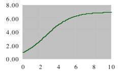
2. 𝑁 = 4, 𝐴 = 0.333, 𝑏 = 4; 4/(1+0.333*4^-x)

3. 𝑁 = 10, 𝐴 = 4, 𝑏 = 0 3; 10/(1+4*0.3^-x)

4. 𝑁 = 100, 𝐴 = 5, 𝑏 = 0 5; 100/(1+5*0.5^-x)
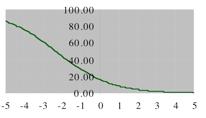
5. 𝑁 = 4, 𝐴 = 7, 𝑏 = 1 5; 4/(1+7*1.5^-x)

6. 𝑁 = 8.5, 𝐴 = 3.25, 𝑏 = 1.05; 8.5/(1+3.25*1.05^-x)

7. 𝑁 = 200, the limiting value. 10 = 𝑓 (0) = 𝑁 /(1 + 𝐴) = 200/(1 + 𝐴) , so 𝐴 = 19. For small values of 𝑥, 𝑓 (𝑥) ≈ 10𝑏 𝑥 ; to double with every increase of 1 in 𝑥 we must therefore have 𝑏 = 2. This gives 𝑓 (𝑥) = 200 1 + 19(2 𝑥)
8. 𝑁 = 10, the limiting value. 1 = 𝑓 (0) = 𝑁 /(1 + 𝐴) = 10/(1 + 𝐴) , so 𝐴 = 9. For small values of 𝑥, 𝑓 (𝑥) ≈ 𝑏 𝑥 ; to grow by 50% with every increase of 1 in 𝑥 we must therefore have 𝑏 = 1.5. This gives 𝑓 (𝑥) = 10 1 + 9(1.5) 𝑥 .
9. 𝑁 = 6, the limiting value. 3 = 𝑓 (0) = 𝑁 /(1 + 𝐴) = 6/(1 + 𝐴) , so 𝐴 = 1. 4 = 𝑓 (1) = 6/(1 + 𝑏 1) , 1 + 𝑏 1 = 6/4 = 3/2, 𝑏 1 = 1/2, 𝑏 = 2. So, 𝑓 (𝑥) = 6 1 + 2 𝑥 .
10. 𝑁 = 4, the limiting value. 1 = 𝑓 (0) = 𝑁 /(1 + 𝐴) = 4/(1 + 𝐴) , so 𝐴 = 3 2 = 𝑓 (1) = 4/(1 + 3𝑏 1) , 1 + 3𝑏 1 = 4/2 = 2, 𝑏 1 = 1/3, 𝑏 = 3. So, 𝑓 (𝑥) = 4 1 + 3(3 𝑥)
11. B: The limiting value is 9, eliminating (A). The initial value is 2 = 9/(1 + 3 5), not 9/(1 + 0 5), so the answer is (B), not (C).
12. A: The limiting value is 8, eliminating (C). The initial value is 1 = 8/(1 + 7) as in (A).
13. B: The graph decreases, so 𝑏 < 1, eliminating (C). The 𝑦-intercept is 2 = 8/(1 + 3) as in (B).
14. C: The graph decreases, so 𝑏 < 1, eliminating (A). The 𝑦-intercept is 2.5 = 10/(1 + 3) as in (C).
15. C: The initial value is 2, as in (A) or (C). If 𝑏 were 5, an increase in 1 in 𝑥 would multiply the value of 𝑓 (𝑥) by approximately 5 when 𝑥 is small. However, increasing 𝑥 from 0 to 10 does not quite double the value. Hence 𝑏 must be smaller, as in (C).
16. C: The initial value is 2, as in (A) or (C). If 𝑏 were 15, an increase in 1 in 𝑥 would multiply the value of 𝑓 (𝑥) by approximately 15 when 𝑥 is small. However, increasing 𝑥 from 0 to 20 does not quite double the value. Hence 𝑏 must be smaller, as in (C).
+ 2 4(1 04) 𝑥
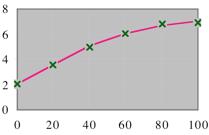
+ 2 5(1 04) 𝑥


20. 𝑦 = 75 1 + 1 5(0 980) 𝑥
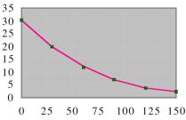
AApppplliiccaattiioonnss
21. a. We can eliminate (B) and (D) because 𝑏 = 0 8 is less than 1, giving a decreasing function of 𝑡. The value 𝑁 = 2 0 in (C) predicts a leveling-off value of around 2%, which is clearly too small. Thus, we are left with choice (A).
b. The logistic curve is steepest when 𝑡 = ln 𝐴 ln 𝑏 . This occurs when 𝑡 = ln 8 6 ln 1 8 ≈ 3 7 years since 2000; during 2003.
22. a. We can eliminate (D) because 𝑏 = 0 8 is less than 1, giving a decreasing function of 𝑡. The leveling-off value in the graph is around 𝑁 = 1, 300, so we can eliminate (A) and (C) Thus, we are left with choice (B).
b. The logistic curve is steepest when 𝑡 = ln 𝐴 ln 𝑏 . This occurs when 𝑡 = ln 4 2 ln 1 7 ≈ 2 7 years since 2000; during 2002.
23. a. We can eliminate (C) because 𝑏 = 0 8 is less than 1, giving a decreasing function of 𝑡. We can eliminate (D) because 𝑏 = 2 0, indicating a rate of growth of 100% per year—far faster than suggested by the data. The value 𝑁 = 300 in (B) predicts a leveling-off value of around 300,000 articles, which is clearly too small. Thus, we are left with choice (A).
b. 1985 is in the initial period of the model, when the rate of growth is governed by exponential growth. Since 𝑏 = 1.04, the rate of growth is 4% per year.
24. a. We can eliminate (B) because 𝑏 = 0 98 < 1, giving a decreasing function of 𝑡. We can eliminate (A) because 𝑏 = 1 50, indicating that the curve initially behaves like an exponential function with base 1.50, increasing by half each year. This is not what is suggested in the data. The value 𝑁 = 300 in (C) predicts a horizontal asymptote of 300,000, which is clearly too small. Thus, we are left with choice (D).
b. 1985 is in the initial period of the model, when the rate of growth is governed by exponential growth. Since 𝑏 = 1 02, the rate of growth is 2% per year.
25. a. For the extremely wealthy we look at large values of 𝑥, where 𝑃 (𝑥) is close to 𝑁 = 95 0%.
b. 𝑃 (𝑥) ≈ [95 0/(1 + 2 78)](1 064) 𝑥 ≈ 25 13(1 064) 𝑥
c. Set 𝑃 (𝑥) = 50 and solve for 𝑥:
50 = 95 0/[1 + 2 78(1 064) 𝑥]
1 + 2 78(1 064) 𝑥 = 95 0/50 = 1 9
𝑥 = log[(1 9 1)/2 78]/ log(1 064) ≈ 18 18, representing approximately $18,000.
SSoolluuttiioonnss SSeeccttiioonn 22..44
26. a. For the extremely wealthy we look at large values of 𝑥, where 𝑃 (𝑥) is close to 𝑁 = 86 2%.
b. 𝑃 (𝑥) ≈ [86 2/(1 + 2 49)](1 054) 𝑥 ≈ 24 70(1 054) 𝑥
c. Set 𝑃 (𝑥) = 50 and solve for 𝑥:
50 = 86 2/[1 + 2 49(1 054) 𝑥]
1 + 2 49(1 054) 𝑥 = 86 2/50 = 1 724
𝑥 = log[(1 724 1)/2 49]/ log(1 054) ≈ 23 49, representing approximately $23,000.
27. 𝑁 = 10, 000, the susceptible population. 1, 000 = 10, 000/(1 + 𝐴), so 𝐴 = 9. In the initial stages, the rate of increase was 25% per day, so 𝑏 = 1 25. Thus, 𝑁 (𝑡) = 10, 000 1 + 9(1 25) 𝑡 𝑁 (7) ≈ 3, 463 cases.
28. 𝑁 = 10, 000, the susceptible population. 1 = 10, 000/(1 + 𝐴), so 𝐴 = 9, 999. In the initial stages, the rate of increase was 40% per day, so 𝑏 = 1 4. Thus, 𝑁 (𝑡) = 10, 000 1 + 9, 999(1 4) 𝑡 ; 𝑁 (21) ≈ 1, 049 cases.
29. 𝑁 = 3, 000, the total available market. 100 = 3, 000/(1 + 𝐴), so 𝐴 = 29. Sales are initially doubling every 5 days, so 𝑏 5 = 2, or 𝑏 = 2 1/5. Thus, 𝑁 (𝑡) = 3, 000 1 + 29(2 1/5) 𝑡 . Set 𝑁 (𝑡) = 700 and solve for 𝑡:
700 = 3, 000/[1 + 29(2 1/5) 𝑡], 1 + 29(2 1/5) 𝑡 = 30/7, (2 1/5) 𝑡 = 23/(29 × 7), 𝑡 = log[23/(29 × 7)]/ log(2 1/5) ≈ 16 days.
30. 𝑁 = 100, the saturation level. 2 = 100/(1 + 𝐴), so 𝐴 = 49. Sales are initially doubling every 2 years, so 𝑏 2 = 2, or 𝑏 = √2 . Thus, 𝑁 (𝑡) = 100 1 + 49(√2) 𝑡 . Set 𝑁 (𝑡) = 50 and solve for 𝑡:
50 = 100/[1 + 49(√2) 𝑡] , 1 + 49(√2) 𝑡 = 2 , (√2) 𝑡 = 1/49 , 𝑡 = log(1/49)/ log(√2) ≈ 11 years, or sometime in 2004.
31. a. Following Example 2, if using Excel, start with initial rough estimates of 𝑁 , 𝐴, and 𝑏 𝑁 = leveling-off value
≈ 10, 000. (Guessing high because the number of articles is still increasing.) 𝑏 = 1.02 (based roughly on the increase from 1985 to 1990). 𝐴: Use 𝑦-intercept = 𝑁 /(1 + 𝐴) and estimate the 𝑦-intercept as 150:
150 = 10, 000 1 + 𝐴
1 + 𝐴 = 10, 000/150 ≈ 67
So, 𝐴 ≈ 66. Solver then gives the following solution:
𝑁 ≈ 9, 790, 𝐴 ≈ 69 0, 𝑏 ≈ 1 04
Thus, the regression model is
SSoolluuttiioonnss SSeeccttiioonn 22..44
𝐴(𝑡) = 9, 790 1 + 69.0(1.04) 𝑡 .
The model predicts that the number will level off around 𝑁 = 9, 790 thousand articles. Note: The coefficients you get will vary depending on the initial guesses you use.
b. 𝐴(28) = 9, 790 1 + 69 0(1 04) 28 ≈ 408 thousand articles.
32. a. Following Example 2, if using Excel, start with initial rough estimates of 𝑁 , 𝐴, and 𝑏 𝑁 = leveling-off value ≈ 10, 000. (Guessing high because the number of articles is still increasing.) 𝑏 = 1.02 (based roughly on the increase from 1985 to 1990). 𝐴: Use 𝑦-intercept = 𝑁 /(1 + 𝐴) and estimate the 𝑦-intercept as 200:
200 = 10, 000 1 + 𝐴
1 + 𝐴 = 10, 000/200 ≈ 50
So, 𝐴 ≈ 49. Solver then gives the following solution:
𝑁 ≈ 10, 000, 𝐴 ≈ 55, 𝑏 ≈ 1 02
Thus, the regression model is 𝐴(𝑡) = 10, 000 1 + 55(1.02) 𝑡 .
The model predicts that the number will level off around 𝑁 = 10, 000 thousand articles. Note: The coefficients you get will vary depending on the initial guesses you use.
b. 𝐴(28) = 10, 000 1 + 55(1 02) 28 ≈ 307 thousand articles.
33. a. Following Example 2, if using Excel, start with initial rough estimates of 𝑁 , 𝐴, and 𝑏. (Their exact value is not important.) 𝑁 = leveling-off value ≈ 1, 100. 𝑏 = 1.1 (slightly greater than 1, since 𝑁 is increasing with 𝑡). 𝐴: Use 𝑦 -intercept = 𝑁 /(1 + 𝐴):
767 = 1, 100 1 + 𝐴
1 + 𝐴 = 1, 100/767 ≈ 1 4
So, 𝐴 ≈ 0.4. Solver then gives the following solution:
𝑁 ≈ 1, 090, 𝐴 ≈ 0 410, 𝑏 ≈ 1 09 Thus, the regression model is
𝐵(𝑡) = 1, 090 1 + 0 410(1 09) 𝑡
The model predicts that the number will level off around 𝑁 = 1, 090 teams.
b. The logistic curve is steepest when 𝑡 = ln 𝐴 ln 𝑏 . This occurs when 𝑡 = ln 0 410 ln 1 09 ≈ 10.3. This means that, according to the model, the number of teams was rising fastest about 10.3 years prior to 1990; that is, sometime during 1979.
c. Since the coefficient of 𝑏 is 1.09, the number of men's basketball teams was growing by about 9% per year in the past, well before 1979.
34. a. Following Example 2, if using Excel, start with initial rough estimates of 𝑁 , 𝐴, and 𝑏. (Their exact value is not important.) 𝑁 = leveling-off value ≈ 1, 050. 𝑏 = 1.1 (slightly greater than 1, since 𝑁 is increasing with 𝑡). 𝐴: Use 𝑦 -intercept = 𝑁 /(1 + 𝐴):
SSoolluuttiioonnss SSeeccttiioonn 22..44
782 = 1, 050
1 + 𝐴
1 + 𝐴 = 1, 050/782 ≈ 1 3
So, 𝐴 ≈ 0.3. Solver then gives the following solution:
𝑁 ≈ 1, 080, 𝐴 ≈ 0 401, 𝑏 ≈ 1 12
Thus, the regression model is
𝐵(𝑡) = 1, 080
1 + 0.401(1.12) 𝑡 .
The model predicts that the number will level off around 𝑁 = 1, 080 teams.
b. The logistic curve is steepest when 𝑡 = ln 𝐴 ln 𝑏 . This occurs when 𝑡 = ln 0 401 ln 1 12 ≈ 8.06. This means that, according
to the model, the number of teams was rising fastest about 8.06 years prior to 1990; that is, sometime during 1981.
c. Since the coefficient of 𝑏 is 1.12, the number of women's basketball teams was growing by about 12% per year in the past, well before 1981.
35. For a limiting value of 4.5 million, we take 𝑁 = 4, 500. Here is the set of values (𝑥, 𝑁 /𝑦 1) with 𝑁 = 4, 500:
The exponential regression equation is 𝑦 ≈ 1.1466(0.96551) 𝑥 so that 𝐴 = 1.1466. 𝑏 1 = 0.96551, giving 𝑏 = 1/0 96551 ≈ 1 0357. Thus the logistic model is 𝑦 = 4, 500 1 + 1.1466(1.0357) 𝑡 , To predict when 𝑦 = 4, 000, we set 4, 000 = 4, 500 1 + 1 1466(1 0357) 𝑡 and solve for 𝑡: 1 + 1 1466(1 0357) 𝑡 = 4, 500 4, 000 = 1 125 so (1 0357) 𝑡 = (1 125 1)/1 1466 ≈ 0 1090, giving
𝑡 = ln(0 1090) ln(1.0357) ≈ 63, or 2013.
36. For a limiting value of 110,000 million, we take 𝑁 = 110. Here is the set of values (𝑥, 𝑁 /𝑦 1) with 𝑁 = 110: 𝑥 0
The exponential regression equation is 𝑦 ≈ 2.3596(0.92877) 𝑥 so that 𝐴 = 2.3596 𝑏 1 = 0.92877, giving 𝑏 ≈ 1.07670 Thus the logistic model is
𝑦 = 110 1 + 2.3596(1.0767) 𝑡 .
To predict when 𝑦 = 80, we set 80 = 110 1 + 2.3596(1.0767) 𝑡 and solve for 𝑡:
1 + 2 3596(1 0767) 𝑡 = 110 80 = 1 12
so (1 0767) 𝑡 = (1 125 1)/2 3596 ≈ 0 0530, giving
𝑡 = ln(0 0530) ln(1.0767) ≈ 40, or 1990.
CCoommmmuunniiccaattiioonn aanndd rreeaassoonniinngg eexxeerrcciisseess
37. Just as diseases are communicated via the spread of a pathogen (such as a virus), new technology is communicated via the spread of information (such as advertising and publicity). Further, just as the spread of a disease is ultimately limited by the number of susceptible individuals, so the spread of a new technology is ultimately limited by the size of the potential market.
38. Exponential functions grow large without bound and fail to take into account the limited size of the susceptible population. Logistic functions correctly predict a slowing in the spread of an epidemic as the number of cases grows toward the total susceptible population.
39. It can be used to predict where the sales of a new commodity might level off.
40. Answers may vary. The number of subprime mortgages (Exercise 21) or the value of subprime debt (Exercise 22) should not be expected to remain near the fixed level predicted by a regression model. (In fact, these numbers started to decline in mid-2008.) Similarly, the number of research articles written in Europe or in the U.S. for a journal (Exercises 23 and 24) cannot be expected to remain at near-constant level from some point on.
41. The curve is still a logistic curve, but decreases when 𝑏 > 1 and increases when 𝑏 < 1.
42. If 𝐴 = 0, then the function is constant: 𝑃 (𝑡) = 𝑁 . If 𝐴 < 0, then the function will have a vertical asymptote at 𝑡 = ln 𝐴/ ln 𝑏; to the left of the asymptote it approaches 0; to the right it decreases to 𝑁
43. Substituting 𝑡 = ln 𝐴 ln 𝑏 in the formula for 𝑦 gives
ln𝑏
= 1 𝐴 , so
= 𝑁 1 + 𝐴(1/𝐴) = 𝑁 1 + 1 = 𝑁 /2
44. For 𝑡 = ln 𝐴/ ln 𝑏 to be positive, the numerator and denominator must have the same sign. Case 1: Both positive: In this case, both 𝐴 and 𝑏 must be > 1
Case 2: Both negative: In this case, both 𝐴 and 𝑏 must be < 1
For 𝑡 = ln 𝐴/ ln 𝑏 to be negative, the numerator and denominator must have opposite sign. That is, either 𝐴 > 1 and 𝑏 < 1, or 𝐴 < 1 and 𝑏 > 1
For 𝑡 = ln 𝐴/ ln 𝑏 to be zero, ln 𝐴 must be zero; that is, 𝐴 = 1
SSoolluuttiioonnss CChhaapptteerr 22 RReevviieeww CChhaapptteerr 22 RReevviieeww
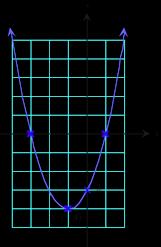
1. 𝑎 = 1, 𝑏 = 2, 𝑐 = 3, so 𝑏/(2𝑎) = 1; 𝑓 ( 1) = 4 , so the vertex is ( 1, 4) 𝑦-intercept: 𝑐 = 3
𝑥 2 + 2𝑥 3 = (𝑥 + 3)(𝑥 1), so the 𝑥-intercepts are 3 and 1 𝑎 > 0, so the parabola opens upward.
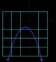
2. 𝑎 = 1, 𝑏 = 1, 𝑐 = 1, so 𝑏/(2𝑎) = 1/2; 𝑓 ( 1/2) = 3/4 , so the vertex is ( 1/2, 3/4) 𝑦-intercept: 𝑐 = 1
𝑏 2 4𝑎𝑐 = 3 < 0, so there are no 𝑥-intercepts. 𝑎 < 0, so the parabola opens downward.
3. For every increase in 𝑥 by 1 unit, the value of 𝑓 is multiplied by 1/2, so 𝑓 is exponential. Since 𝑓 (0) = 5 , the exponential model is 𝑓 (𝑥) = 5(1/2) 𝑥 , or 5(2 𝑥) 𝑔(2) = 0, whereas exponential functions are never zero, so 𝑔 is not exponential.
4. The values of 𝑓 decrease by 2 for every increase in 𝑥 by 1 unit, so 𝑓 is linear (not exponential). For every increase in 𝑥 by 1 unit, the value of 𝑔 is multiplied by 2, so 𝑔 is exponential. Since 𝑔(0) = 3, the exponential model is 𝑔(𝑥) = 3(2 𝑥)
5. We use the table of values shown on the left to obtain the graph shown on the right:

6. We use the table of values shown on the left to obtain the graph shown on the right:

7. The technology formulas for the two functions are TI-83/84 Plus: e^x; e^(0.8*x)
Excel: =EXP(x); =EXP(0.8*x) Technology gives us the following graphs:
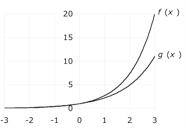
8. The technology formulas for the two functions are TI-83/84 Plus and Excel: 2*1.01^x ; 2*0.99^x Technology gives us the following graphs:

SSoolluuttiioonnss CChhaapptteerr 22 RReevviieeww
13. Use 𝐴 = 𝑃 𝑒 𝑟𝑡; 𝑃 = 3, 000, 𝑟 = 0 03; 𝑡 = 5. So, 𝐴 = 3, 000𝑒 0.15 ≈ $3, 485 50
14. Use 𝐴 = 𝑃 𝑒 𝑟𝑡; 𝑃 = 10, 000, 𝑟 = 0 025; 𝑡 = 10. So, 𝐴 = 10, 000𝑒 0.25 ≈ $12, 840 25
15. Increasing 𝑥 by one half unit triples the value of 𝑓 . Therefore, increasing 𝑥 by 1 unit multiplies the value of 𝑓 by 9, giving 𝑏 = 9 𝐴 = 𝑓 (0) = 4 5 . Therefore, 𝑓 (𝑥) = 𝐴𝑏 𝑥 = 4 5(9 𝑥)
16. Increasing 𝑥 by 1 unit decreases the value of 𝑓 by 75%. That is, it reduces the value of 𝑓 to 25% of its original value. Therefore, 𝑏 = 0 25 𝐴 = 𝑓 (0) = 5 . Therefore, 𝑓 (𝑥) = 𝐴𝑏 𝑥 = 5(0 25 𝑥)
17. 2 = 𝐴𝑏 1 and 18 = 𝐴𝑏 3. Dividing, 𝑏 2 = 9, so 𝑏 = 3. Then 2 = 3𝐴, so 𝐴 = 2/3: 𝑓 (𝑥) = 2 3 3 𝑥
18. 10 = 𝐴𝑏 1 and 5 = 𝐴𝑏 3. Dividing, 𝑏 2 = 1/2, so 𝑏 = 1/√2 . Then 10 = 𝐴/√2 , so 𝐴 = 10√2 : 𝑓 (𝑥) = 10√2( 1 √2 ) 𝑥
19. We use the following table of values:
Graphing these gives the following curves:
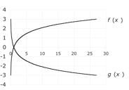
20. We use the following table of values:
Graphing these gives the following curves:
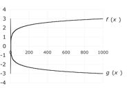
21. 𝑄0 = 5 (given)
𝑡ℎ 𝑘 = ln 2
100𝑘 = ln 2
𝑘 = (ln 2)/100 ≈ 0 00693
𝑄 = 𝑄0 𝑒 𝑘𝑡 = 5𝑒 0.00693𝑡
23. 𝑄0 = 2.5 (given)
𝑡𝑑 𝑘 = ln 2
2𝑘 = ln 2
𝑘 = (ln 2)/2 ≈ 0.347 𝑄 = 𝑄0 𝑒 𝑘𝑡 = 2 5𝑒 0.347𝑡
25. 3, 000 = 2, 000(1 + 0.04/12) 12𝑡
𝑡 = [log(3/2)/ log(1 + 0 04/12)]/12 ≈ 10 2 years
26. 3, 000 = 2, 000(1 + 0.0675/365) 365𝑡
𝑡 = [log(3/2)/ log(1 + 0 0675/365)]/365 ≈ 6 years
27. 3, 000 = 2, 000𝑒 0.0375𝑡
𝑡 = ln(3/2)/0.0375 ≈ 10.8 years
28. 1, 200 = 1, 000(1 + 1/4) 4𝑡 = 1, 000(1 25 4𝑡)
𝑡 = [log(1, 200/1, 000)/ log(1.25)]/4 ≈ 0.2 years
22. 𝑄0 = 10, 000 (given) 𝑡ℎ 𝑘 = ln 2
5𝑘 = ln 2
𝑘 = (ln 2)/5 ≈ 0 139 𝑄 = 𝑄0 𝑒 𝑘𝑡 = 10, 000𝑒 0.139𝑡
24. 𝑄0 = 10, 000 (given) 𝑡𝑑 𝑘 = ln 2
15𝑘 = ln 2
𝑘 = (ln 2)/15 ≈ 0.0462 𝑄 = 𝑄0 𝑒 𝑘𝑡 = 10, 000𝑒 0.0462𝑡
29. 𝑁 = 900 is given, 100 = 900/(1 + 𝐴) gives 𝐴 = 8, initially increasing 50% per unit increase in 𝑥 gives 𝑏 = 1 5:
𝑓 (𝑥) = 900 1 + 8(1.5) 𝑥
30. 𝑁 = 25 is given, 5 = 25/(1 + 𝐴) gives 𝐴 = 4, 𝑏 = 1.1 is given in the initial exponential form:
𝑓 (𝑥) = 25 1 + 4(1.1) 𝑥 .
31. 𝑁 = 20 is given, 20/(1 + 𝐴) = 5, so 𝐴 = 3, decreasing at a rate of 20% per unit of 𝑥 near 0 means
𝑏 = 1 0 2 = 0 8:
𝑓 (𝑥) = 20 1 + 3(0 8) 𝑥
32. 𝑁 ≈ 10 and 𝑏 = 0 8 are given, and for small 𝑥, 𝑁 /(1 + 𝐴) = 10/(1 + 𝐴) = 2, so 𝐴 = 4, giving
𝑓 (𝑥) = 10 1 + 4(0 8) 𝑥
33. a. The largest volume will occur at the vertex: 𝑏/(2𝑎) = 0 085/(2 × 0 000005) ≈ $8, 500 per month; substituting 𝑐 = 8, 500 gives ℎ = an average of approximately 2,100 hits per day.
b. Solve ℎ = 0 using the quadratic formula: 𝑐 ≈ $29, 049 per month (the other solution given by the quadratic formula is negative).
c. The fact that 0 000005, the coefficient of 𝑐 2, is negative.
34. a. Since 𝑡 is time in years since the start of 2000 and the data are from the start of 2001 to the end of 2003, the domain is 1 ≤ 𝑡 ≤ 4, or [1, 4].
b. The growth rate is a minimum at the vertex:
𝑡 = 𝑏 2𝑎 = 6 4 = 1.5, midway through 2001.
c. A zero rate of growth would correspond to an intercept of the 𝑡-axis. However, the discriminant
𝑏 2 4𝑎𝑐 = 36 4(2)(12) = 60 is negative, so there are no 𝑡-intercepts, and hence no zero rate of growth.
d. The fact that the coefficient of 𝑡 2 is positive.
e. No. What was decreasing was the number of new broadband users. Put another way, the number of broadband users was growing at a declining rate in the first half of 2001.
f. The beginning of 2013 is 𝑡 = 13;
𝑛(13) = 2(13) 2 6(13) + 12 = 272 million new users per year at the start of 2013
𝑛(14) = 2(14) 2 6(14) + 12 = 320 million new users per year at the start of 2014. These numbers are unreasonably large (recall that they represent new users per year). In fact, their sum exceeds the entire U.S. population.
35. a. 𝑅 = 𝑝𝑞 = 60𝑝 2 + 950𝑝. The maximum revenue occurs at the vertex: 𝑝 = 𝑏/(2𝑎) = 950/(2 × 60) = $7.92 per novel. At that price the monthly revenue is 𝑅 = $3, 760 42
b. 𝐶 = 900 + 4𝑞 = 900 + 4( 60𝑝 + 950) = 240𝑝 + 4, 700, so
𝑃 = 𝑅 𝐶 = 60𝑝 2 + 950𝑝 ( 240𝑝 + 4, 700) = 60𝑝 2 + 1, 190𝑝 4, 700. The maximum monthly profit occurs at the vertex: 𝑝 = 𝑏/(2𝑎) = 1, 190/(2 × 60) = $9 92 per novel. At that price, the monthly profit is 𝑃 = $1, 200 42
36. a. Demand Function: The given points are (𝑝, 𝑞) = (0, 2, 000) and (0.10, 1, 000).
Slope: 𝑚 = 𝑞2 𝑞1 𝑝2 𝑝1 = 1, 000 2, 000 0 10 0 = 10, 000
Intercept: 𝑏 = 2, 000
SSoolluuttiioonnss CChhaapptteerr 22 RReevviieeww
Thus, the demand equation is
𝑞 = 𝑚𝑝 + 𝑏 = 10, 000𝑝 + 2, 000
b. Revenue = 𝑝𝑞 = 𝑝( 10, 000𝑝 + 2, 000) = 10, 000𝑝 2 + 2, 000𝑝. The maximum revenue occurs at the vertex:
𝑝 = 𝑏/(2𝑎) = 2, 000/(20, 000) = $0 1, or 10¢ per newspaper. At that price the monthly revenue is 𝑅 = 10, 000(0.1) 2 + 2, 000(0.1) = $100.
c. 𝐶 = 200 + 0 04𝑞 = 200 + 0 04( 10, 000𝑝 + 2, 000) = 400𝑝 + 280, so 𝑃 = 𝑅 𝐶 = 10, 000𝑝 2 + 2, 000𝑝 ( 400𝑝 + 280) = 10, 000𝑝 2 + 2, 400𝑝 280
The maximum monthly profit occurs at the vertex: 𝑝 = 𝑏/(2𝑎) = 2, 400/20, 000 = $0.12 per newspaper. At that price, the monthly profit is 𝑃 = 10, 000(0 12) 2 + 2, 400(0 12) 280 = 136, a loss of $136.
37. a. 1997 corresponds to 𝑡 = 0, and so the harvest was 𝑛 = 9 1(0 81 0) = 9 1 million pounds. The value of the base 𝑏 = 0.81 of the exponential model tells us that the value each year is 0.81 times, or 81% of the value the previous year.
In other words, the value decreases by 100 81 = 19% each year.
b. 2013 corresponds to 𝑡 = 16, and
𝑛(16) = 9.1(0.81 16) ≈ 0.31, or about 310,000 pounds.
38. Let 𝑆 be the stock price and 𝑡 be the time in hours since the IPO. Model the stock price by 𝑆 = 𝐴𝑏 𝑡. Then
𝐴 = 10, 000 and 𝑏 3 = 2 (since the stock is doubling in price every 3 hours), so 𝑏 = 2 1/3. After 8 hours,
𝑆 = 10, 000(2 1/3) 8 = $63, 496.04.
39. The model for the lobster harvest from Exercise 37 is 𝑛(𝑡) = 9 1(0 81 𝑡) million pounds. We need to find the value of 𝑡 when it first dips below 200,000, which is 0.2 million pounds:
0.2 = 9.1(0.81 𝑡)
0.2/9.1 = 0.81 𝑡
log(0 2/9 1) = 𝑡 log(0 81)
𝑡 = log(0 2/9 1)/ log(0 81) ≈ 18 1.
Thus, the harvest is still above 200,000 lobsters at 𝑡 = 18 (2015), but will be below 200,000 at 𝑡 = 19 (2016).
40. Solve 50, 000 = 10, 000(2 𝑡/3): 𝑡 = 3log 5/ log 2 ≈ 7 0 hours.
41. In 2010 (𝑡 = 13), the harvest was 9 1(0 81 13) ≈ 0 5880. From that point on, the model is 0.5880(1 24) 𝑡 where 𝑡 is now time in years since 2010. In 2013, the size of the harvest is 0.5880(1 24) 3 ≈ 1 12 million pounds.
42. After 10 hours the stock is worth 10, 000(2 10/3) = $100, 793 68. From this level it follows a new exponential curve with 𝐴 = 100, 793 68 and 𝑏 4 = 2/3 (it loses 1/3 of its value every 4 hours), hence 𝑏 = (2/3) 1/4. Now solve
SSoolluuttiioonnss CChhaapptteerr 22 RReevviieeww
10, 000 = 100, 793.68(2/3) 𝑡/4 for 𝑡 = 4log(10, 000/100, 793.68)/ log(2/3) ≈ 22.8. Adding the first 10 hours, the stock will be worth $10,000 again 32.8 hours after the IPO.
43. We use the data shown in the following table:
The regression model is Excel: 𝑛(𝑡) = 9 5841𝑒 0 224𝑡 = 9 5841(𝑒 0 224) 𝑡 ≈ 9 5841(0 7993) 𝑡
TI-83/84 Plus and Website: 9.5841(0.79967) 𝑡
Rounding to 2 digits gives 𝑛(𝑡) = 9 6(0 80 𝑡) million pounds of lobster.
44. We use the data shown in the following table:
The regression model is Excel: 𝑃 (𝑡) = 1 0321𝑒 0.2276𝑡 = 1 0321(𝑒 0.2276) 𝑡 ≈ 1 03(1 26) 𝑡
TI-83/84 Plus and Web Site: 𝑦 = 1 03206(1 25564 𝑡)
Rounding to 2 digits gives 𝑃 (𝑡) = 1 03(1 26) 𝑡. To predict numerically when the price passes $10 we can use a table of values in the TI-83/84 Plus, Excel, or the Website with y = 1.03*(1.26^x)
1.03*(1.26^x)
1.03
Thus, the stock price first passes $10 at the end of the 10th hour.
45. C: (A) is true because 𝐿1 = 𝐿0 𝑒 1/𝑡 < 𝐿0 . (B) is true because 𝐿3𝑡 = 𝐿0 𝑒 3 > 0. (D) is true because increasing 𝑡 decreases 𝑥/𝑡, which increases 𝑒 𝑥/𝑡 (makes it closer to 1), hence increases 𝐿𝑥 for every 𝑥. (E) is true because 𝑒 𝑥/𝑡 is never 0. On the other hand, (C) is false because 𝐿𝑡 = 𝐿0 𝑒 1 ≈ 0.37𝐿0 < 𝐿0 /2.
46. a. The given function has the form Constant + logistic function. The logistic function part levels off at 𝑁 = 4, 470.
Therefore, adding the constant gives a leveling of at 4, 470 + 6, 050 = 10, 520
b. We solve
10, 000 = 6, 050 + 4, 470 1 + 14(1.73 𝑡)
3, 950 = 4, 470 1 + 14(1 73 𝑡)
1 + 14(1 73 𝑡) = 4, 470/3, 950
14(1 73 𝑡) = 4, 470/3, 950 1
1 73 𝑡 = (4, 470/3, 950 1)/14
𝑡 log(1.73) = log((4, 470/3, 950 1)/14)
𝑡 = log((4, 470/3, 950 1)/14)/ log(1 73) ≈ 8 5, about 8.5 weeks.
c. Sales are rising most rapidly when 𝑡 = ln 𝐴/ ln 𝑏 = ln 14/ ln 1 73 ≈ 5 to the nearest week.
SSoolluuttiioonnss CChhaapptteerr 22 CCaassee SSttuuddyy
CChhaapptteerr 22 CCaassee SSttuuddyy
1. If we take 𝑡 = 0 to represent 1900 as in the text and do an exponential regression directly, we obtain the model 𝑦 ≈ 552, 000𝑒 0.0145𝑡. If we do instead a linear regression of ln 𝑦 versus 𝑡, we get the following regression equation:
ln 𝑦 = 0.0145𝑡 + 13.221. Rewriting this in exponential form gives
𝑦 = 𝑒 0 0145𝑡 + 13 221
= 𝑒 13.221𝑒 0.0145𝑡
≈ 552, 000𝑒 0.0145𝑡 Coefficients rounded to 3 digits
The growth constant is 𝑘 ≈ 0 0145, which is larger than that based on the data from 1900 on: 𝑘 ≈ 0 0139. This suggests that wheat production in the U.S. grew at larger annual percentage after 1950 than before.
2. Using the method described in Section 3 to do logistic regression, we obtain the model
𝑃 (𝑡) ≈ 2, 330, 000 1 + 164(1 09 𝑡) ; SSE ≈ 4 53 × 10 12
The model predicts a leveling off of wheat production around 𝑁 = 2, 330, 000 thousand bushes, which is more-or-less at current production levels!
Graphs:
Logistic:
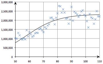
SSE ≈ 4 53 × 10 12
Exponential:
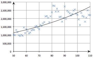
SSE ≈ 8 38 × 10 12
(To compute SSE for the exponential model, we summed the squares of the residuals directly using the model with coefficients to 6 decimal places.) The logistic curve gives a better fit both graphically and in terms of SSE. This suggests that wheat production has already leveled off, vindicating Malthus's pessimistic predictions.
3. Answers will vary, depending on the crop and time period chosen.
4. (𝑡 = 0 represents 1820 in all models, 𝑡 measured in decades.)
Linear model: 𝑃 = 15, 589𝑡 29, 335, 𝑟 2 = 0 94903
Superficially a good fit, but the negative constant term is disturbing as is the nonrandom distribution of the residuals. The data clearly suggest an upward curve, not a straight line.
Quadratic model: 𝑃 = 696 27𝑡 2 + 2, 359 4𝑡 + 10, 352, 𝑟 2 = 0 99901
An excellent fit visually and a high value of 𝑟 2
Exponential: 𝑃 = 14, 417𝑒 0.1771𝑡 , 𝑟 2 = 0 96348
Not as good a fit as the quadratic model. From the graph it is clear that the exponential model grows too slowly at first and too quickly after about 1930 or so. Conclusion: The quadratic model is definitely the best of the three.
