Chapter2 ORGANIZATIONAND DESCRIPTIONOFDATA
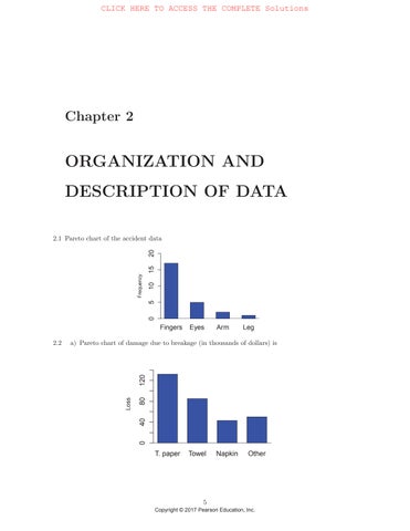
2.1Paretochartoftheaccidentdata
Frequency05101520
2.2a)Paretochartofdamageduetobreakage(inthousandsofdollars)is
b)Percentofthelossthatoccursinmakingtoiletpaperis
c)Percentofthelossthatoccursinmakingtoiletpaperorhandtowelsis
2.3Thedotdiagramoftheenergyis
2.4Thedotdiagramofthepaperstrengthdatais
110115120125130135140
2.5Thedotdiagramofthesuspendedsolidsdatarevealsthatonereading,65ppm,isverylarge.Other readingstakenataboutthesametime,butnotgivenhere,confirmthatthewaterqualitywasbadat thattime.Thatis,65isareliablenumberforthatday.
2.6Thedotdiagramofthetimesforthepoweroutagesshowsonelargevalue,10.0hours.
Time(hours)
2.7(a)
Timebetweenarrivals(sec)
(b)Theoneextremelylargegapbetween2.0and7.3secondsisanoutlier.Thiscouldbedueto neutrinosthatweremissedorthepossibilitythattwoexplosionsoccurred.
2.8(a)Theclassmarksare150.0,170.0,190.0,210.0,230.0and250.0.
(b)Theclassintervalis20.
2.9(a)Yes.Thisisthenumberofobservationsintheclass[140.0,160.0).
(b)No.Itisnotpossibletodeterminehowmanyspecimenshavebreakingstrength160.
(c)Yes.Thisisthetotalnumberofobservationsinthetwoclasses[220.0,240.0) and[240.0,260.0).
(d)No.Itisnotpossibletodeterminehowmanyofthespecimenshavestrength240.
(e)No.Itisnotpossibletodeterminehowmanyofthespecimenshavestrength260.
2.10Thefrequencydistributionisgiveninthetablewheretheright-handendpointisincluded.
Thehistogramis
ClassFrequency
(60, 70]5
(70, 80]11
(80, 90]9
(90, 100]18
(100, 110]6
(110, 120]1
Frequency 60708090100110120
Diameter(nM)
2.11Wefirstconvertthedataintheprecedingexercisetoa“lessthanorequal”distribution.Theogiveis plottedbelow.
Number less than or equal
Diameter(nM)
2.12Thesedatacanbegroupedintothefollowingfrequencydistributionwheretherighthandendpointis excluded:
ClassClass limitsFrequencylimitsFrequency
[1.0, 2.0)10[7.0, 8.0)6
[2 0, 3 0)10[8 0, 9 0)4
[3 0, 4 0)9[9 0, 10 0)4
[4.0, 5.0)11[10.0, 11.0)1
[5 0, 6 0)12[11 0, 12 0)2 [6 0, 7 0)10[12 0, 13 0)1
Thehistogramis
Frequency
2.13Wefirstconvertthedataintheprecedingexercisetoa“lessthan”distribution.
xNo.lessthanxNo.lessthan 1.008.068 2.0109.072 3.02010.076 4.02911.077 5.04012.079 6.05213.080 7.062
Theogiveis 24681012
2.14Afterorderingthedataweobtainthefrequencydistribution.
Temperature(◦ C)Frequency
[1.10, 1.20)1
[1 20, 1 30)11
[1 30, 1 40)16
[1.40, 1.50)15
[1 50, 1 60)4
[1 60, 1 70)3 Total50
Therelativefrequencyhistogramis
2.15Thecumulativefrequenciesforlessthantheupperlimitoftheintervalare
2.16Thefrequencytableis:
2.17Theempiricalcumulativedistributionfunctionis
2.18Theempiricalcumulativedistributionis:
Empirical Distribution
Numberofaccidents
2.19No.Wetendtocompareareasvisually.Theareaofthelargesackisfarmorethandoubletheareaof thesmallsack.Thelargesackshouldbemodifiedsothatitsareaisslightlylessthandoublethatof thesmallsack.
2.20Thepiechartis
2.21Wefirstnotethattheclassesarenotofequallength.Ifthedistributionofthedatawereuniform overasingleintervalcoveringallofthedata,onewouldexpectthatlongerclasseswouldhavehigher counts.Tocorrectforthis,theareaofeachrectangleshouldbeproportionaltotheproportionof observationsintheclass.Ofcourse,whentheclasslengthsareequal,plottingtheheightequaltothe classfrequencyresultsinrectangleswithareaproportionaltothecorrespondingclassproportions.
Theincorrecthistogramis
Thecorrecthistogramusesheight=(relativefrequency)/width.Theheightofthefirstrectangleis (relativefrequency)/width=(3/50)/40=0.0015.
Thiscorrecthistogramis
2.22Thestemandleafdisplayis:
2.23Thestemandleafdisplayis:
2.24(a)Thedataare:11,12,13,14,15,17,18.
(b)Thedataare:230,230,231,234,236.
(c)Thedataare:203,218,235,257.
(d)Thedataare:3.21,3.23,3.24,3.24,3.27.
2.25Thestem-and-leafdisplayis:LeafUnit=0.010
2.26(a)Thestem-and-leafdisplayis:
(b)Thedataare:
534,534,534,534,535,535,536,536,536,537,538,539,541.
2.27(a)Wouldlikeahighsalary-outlierthatislarge.
(b)Wouldlikeahighscore-outlierthatislarge.
(c)Nearaverage.
2.28(a)Wouldlikefinishearly-outlierthatissmall.
(b)Nearaverage.
2.29Greateronthemean.Itwouldnotinfluencethemedianforsamplesize3ormore.
2.30GreaterontheRange.Itwouldinfluencethevalueoftherangebutnottheinterquartilerangeifthe samplesizeisatleast5.
2.31(a) x =( 6+1 4 3)/4= 3
(b)
(c)Themeanoftheobservationminusspecificationis 3so,onaverage,theobservationsarebelow thespecification.Onaverage,theholesaretoosmall.
2.32(a)
(c)Theaveragedropsbyover40meters,about8%,whentheoneverytallbuildingisexcluded.
2.33(a) x =(35+37+38+34+30+24+13)/7=211/7=30.14mm/min.
(b)Themeandoesnotprovideagoodsummary.Themostimportantfeatureisthedropinperformanceasillustratedintimeorderplotofdistanceversussamplenumber.Itislikelythetipof thelegbecamecoveredwithdebrisagain.Theearlytrialsindicatewhatcanbeexpectedifthis problemcanbeavoided.
2.34(a)Acomputercalculationgives
Samplenumber
Youmayverifythemeanbyfirstshowingthat xi =4265.
(b)Youmayconfirmthecalculationof s byshowingthat x2 i =2041 54so s
2.35No.Thesumofthesalariesmustbeequalto3(175,000)=525,000whichislessthan550,000.This assumesthatallsalariesarenon-negative.Itiscertainlypossibleifnegativesalariesareallowed.
2.36Themeanisindeed85.But,wecommentthat s =15indicatingconsiderablevariationinaverage monthlytemperature.Themedianis86,alsoacomfortabletemperature.
2.37(a)Themeanagreementis:
Consequently, s = √0.0330=0.1817.
2.38(a)Thefollowingtablegivestheobservations,thedeviations,thesquareddeviations,andthesumof thesquareddeviations.
SquaredSquared
SumofSquaredDeviations=.29709
SampleVariance s2 = 29709/9= 03301and s = 1817.
(b)Thesquaredobservationsare: .2500.1600.0016.2025.4225.1600.04000900.3600.2025
Thesumofthesesquaresis1.8891.Thus,
Thus, s = 1817
2.39(a)Themeanoffensivesmellis x = 16 i=1 xi 16 = 53 6 16 =3 35
(b)Theorderedoffensivesmellscoresare
1.01.01.71.92.42.62.73.2
3.33.83.94.35.05.25.36.3
Themedian=(3 2+3 3)/ 2=3 25.
(c)Since16 × (1/4)=4isaninteger, Q1 =(1.9+2.4) /2=2.15and Q3 =(4.3+5.0) /2=4.65.
Theboxplotis 1234567 Offensivesmellscore
2.40(a)Thetableofdata,deviation,anddeviationsquaredis:
Data 61 4 3
Dev. 34 10
Sq.91610
Thesumofthesquareddeviationsis26.Thus, s 2 =26/3=8 667and s =2 94
(b)Thesumoftheobservationsis62.Thesumoftheobservationssquaredis144.Thus,
2.41Themeanis30.91.Thesorteddataare: 29.6,30.3,30.4,30.5,30.7,31.0,31.2,31.2,32.0,32.2
Sincethenumberofobservationsis10(anevennumber),themedianistheaverageofthe5thand6th observationsor(30.7+31.0)/2=30.85.Thefirstquartileisthethirdobservation,30.4,andthethird quartileistheeighthobservation,31.2.
2.42Thetableofdata,deviation,anddeviationsquaredis:
Data97155
Deviation0 26 4 Squares043616
(a)Thedeviations(xi x)addto0+( 2)+6+( 4)=0. (b) (xi x)2 =56.Thus, s2 =56/3=18 66and s =4 32.
2.43Theboxplotisbasedonthefive-numbersummaryofthe n =50temperatures.
2.44(a) x =( 290+ 104+ 207+ 145+ 105+ 124)/6= 974/6= 1623
(b)Wefirstcalculate .2902 + .1042 + .2072 + .1452 + .1052 + .1242 = .18498andthen s 2 =
Consequently, s = √ 005373=0 0733.
2.45(a)Forthenon-leakers x =( 207+ 124+ 062+ 301+ 186+ 124)/6= 16733
(b)Also, .2072 + .1242 + .0622 + .3012 + .1862 + .1242 = .20264so s 2 = 6(.20264) (1.004)2 6 5 = 006928so s = √ 006928= 0832
(c)Themeansarequiteclosetoeachotherandsoarethestandarddeviations.Thesizeofgapdoes notseemtobeconnectedtotheexistenceofleaks.
2.46(a) xi =605.Thus,¯ x =605/20=30 25,and x2 i =20, 663.Hence, s2 =(20 21723 6152 )/(20 19)=124 303.And s =11 15.
(b)Theclasslimits,marks,andfrequenciesareinthefollowingtable:
ClasslimitsClassmarkFrequency 10-1914.53 20-2924.58 30-3934.55 40-4944.53 50-5954.51
Thus, x =(3(14 5)+8(24 5)+5(34 5)+3(44 5)+54 5)/20=30 xi fi =600. x2 i fi =20, 295.Thus, s2 =(20 20, 295 6002 )/(20 19)=120.79.So, s =10.99.
2.47Theclassmarksandfrequenciesare: ClassmarkFrequency
Thus, xi fi =4370, x2 i fi =389, 850.Themeanis4370/50=87.40,and s2 =(389, 850 43702 /50)/(49)=161.47. Copyright©2017PearsonEducation,Inc.
2.48Weusetheclasslimits[1,2),[2,3),...wheretheright-handendpointisexcluded.Theclassmarks andfrequenciesare:
Thus, xi fi =415 0, x2 i fi =2, 722 0.Therefore,themeanis415.0/80=5.188and s2 =(80 · 2, 722.0 415.02 )/(80 79)=7.2049.Thestandarddeviationis s =2.684.Thecoefficientofvariation is v =100 s/x =51 0percent.
2.49FromExercise2.14wehavetheintervalsandfrequencies.Thelasttwocolumnsgivethecalculations ofthebasictotals.
[1 10, 1 20)1.1511.151.3225
[1 20, 1 30)1.251113.7517.1875
[1.30, 1.40)1.351621.6029.1600
[1 40, 1 50)1.451521.7531.5375
[1 50, 1 60)1.5546.209.6100
[1.60, 1.70)1.6534.958.1675 Total5069.4096.9850
Substitutingthetotalsintotheappropriateformulasyields
and
Thecoefficientofvariationisthen
2.51Thenumerator
Thus, sx = csu .
2.53(a)Themedianisthe50/2th=the25thlargestobservation.Thisoccursattheright-handboundary sothemedianis90.Applyingtherule, 90+ 0 18 × 10=90
(b)Thereare80observations.Thereare40observationsinthefirstfourclasses,and40inthelast four.Thus,theestimateforthemedianistheclassboundarybetweenthe4thand5thclass.We coulduse5.0.
2.54(a)Wecanestimatethemeanandthemedianinthiscasesinceweknowtheclassmarksand frequenciesforeachclass.
(b)Wecannotestimatethemeaninthiscase,sincewedonotknowtheclassmarksfortheclasses “lessthan90”and“morethan119”.Wecanestimatethemedian.Itliesinthethirdclass,and weproceedasbefore.
(c)Again,wecannotestimatethemeansincewedonotknowtheclassmarkfortheclass“110or less”.Wealsocannotestimatethemedian,asitalsoliesintheclass“110orless”.
2.55(a)Thereare50observations. Q1 isinthesecondclassand Q3 isinthe4thclass.Thelowerclass boundaryforthe2ndclassis245.Thereare3observationsinthefirstclassand11inthe2nd class.Theclassintervalis40.Thus, Q1 isestimatedby40(50/4 3)/11+245=279.55 Proceedinginasimilarfashiongives325+40(37.5 37)/9=327.22astheestimateof Q3 .Thus, theinterquartilerangeis47.67.
(b)Thereare80observationsand80/4=20whichisontheboundaryofthesecondandthirdclasses sotheestimatefor Q1 is3.00andfor Q3 itis1((60 52)/10+6.00=6.80.
2.56(a)Theaveragesalarypaidtothe30executivesis
(4 · 264,000+15 ·272,000+11 · 269,000)/(4+15+11)=269,833.33.
(b)Themeanfortheentireclassis (22 · 71+18 · 78+10 · 89)/(22+18+10)=77.12.
2.57(a)Theweightedaverageforthestudentis (69+75+56+72+4 78)/8=73.0.
(b)Thecombinedpercentincreasefortheaveragesalariedworkeris: (24 60+33 30+15 40)/(24+33+15)=42.08percent. Copyright©2017PearsonEducation,Inc.
2.58UsingMINITABandtheDESCRIBEcommand,weobtain x and s
(a)Forthedecaytimesdata
NMEANMEDIANSTDEVMINMAX C1500.54950.29450.62420.04102.8630
(b)Fortheinterrequesttimes
NMEANMEDIANSTDEVMINMAX C1501179562481405699578811
2.59(a)Fromtheordereddata,thefirstquartile Q1 =1, 712,themedian Q2 =1, 863andthethird quartile Q3 =2, 061.
(b)Thehistogramis
Strength Frequency
Mean Q2 Q1Q3
10001500200025003000
(c)Forthealuminumdata,wefirstsortthedata. 66.467.768.068.068.368.468.668.8 68.969.069.169.269.369.369.569.5
69.669.769.869.869.970.070.070.1
70.270.370.370.470.570.670.670.8
70.971.071.171.271.371.371.571.6
71.671.771.871.871.972.172.272.3
72.472.672.772.973.173.373.574.2
74.575.3
Thefirstquartile Q1 =69 5,themedian Q2 =70 55andthethirdquartile Q3 =71 80.The histogramis
2.60TheParetochartforcomputerchipsdefectsis
2.61(a)Thefrequencytableofthealuminumalloystrengthdata(right-handendpointexcluded)is
ClasslimitsFrequency
[66 0, 67 5)1
[67 5, 69 0)8
[69.0, 70.5)19
[70 5, 72 0)17
[72.0, 73.5)9
[73 5, 75 9)3
[75 0, 76 5)1
(b)Thehistogram,usingthefrequencytableinpart(a),is
2.62(a)Frequencytableoftheinterrequesttimedata
ClasslimitsFrequency(Relativefrequency)/width
[0, 2500)90.0036
[2500, 5000)130.0052
[5000, 10000)100.0020
[10000, 20000)80.0008
[20000, 40000)80.0004
[40000, 60000)10.0001
[60000, 80000)10.0001
(b)Thehistogram,usingthefrequencytableinpart(a),isgiveninFigure2.1.
2.63(a)Themeanandstandarddeviationfortheearth’sdensitydataare x =5 4835and s =0 19042
(b)Theordereddataare
5.105.275.295.295.305.345.345.365.395.425.445.46
Density
0.0000.0020.004
010305070
Interrequesttime(unit=1,000)
Figure2.1:HistogramforExercise2.62
5.475.535.575.585.625.635.655.685.755.795.85
Thereare n =23observations.Themedianisthemiddlevalue,or5.46.Themustbeatleast 23/4=5.75observationsatorbelow Q1 so Q1 isthe6thlargesvalue. Q1 =5 34.Similarly,there mustbeatleast3(23/4)=17.25observationsatorbelow Q3 so Q3 isthe18thlargestobservation. Q3 =5.63.
(c)Fromtheplotoftheobservationsversustimeorderweseethatthereisnoobvioustrendalthough thereissomesuggestionofanincreaseoverthelasthalfoftheobservations.
Observation
Timeorder
2.64(a)DotdiagramofTube1andTube2observations.
(b)MeanandstandarddeviationforTube1are¯ x1 =0 42and s1 =0 085049
(c)MeanandstandarddeviationforTube2are¯ x2 =0 52857and s2 =0 066440
2.65(a)Theordereddataare
0.320.340.400.400.430.480.57
Sincethereare7observations,themedianisthemiddlevalue.Themedian,maximum,minimum andrangefortheTube1observationsare:
Median=0.40,maximum=0.57,minimum=0.32and range=maximum minimum=0.57 0.32=0.25.
(b)Theordereddataare:
0.470.470.480.510.530.610.63
Andthemedian,maximum,minimumandrangefortheTube2observationsare:
Median=0.51,maximum=0.63,minimum=0.47and range=maximum minimum=0.63 0.47=0.16.
2.66(a)Dotdiagramforthevelocityoflightminus299,700km/sis
1020304050
(b)Themeanforthe(velocityoflight) 299,700isequalto27.545andthemedianisequalto27.
(c)Thevarianceandthestandarddeviationare s2 =100.47and s =10.024
2.67(a)Here,11/4=2 25so Q1 isthe3rdlargestvalue.Thequartilesforthevelocityoflightdataare Q1 =18 0, Q2 =27 0,and Q3 =30 0
(b)Theminimum,maximum,rangeandtheinterquartilerangeare Minimum=12,maximum=48,range=maximum minimum=48 12=36and interquartilerange= Q3 Q1 =30 0 18 0=12 0.
(c)Thebox-plotis
2.68(a)Thedotdiagramforthesuspendedsolidsdatais
10203040506070
Median Mean
Suspendedsolids
(b)Themedian=28.0andthemean=32.182.
(c)Thevarianceandstandarddeviationare s2 =363.76and s =19.073.
2.69(a)Theordereddataare:1214192021282930556363
Thequartilesforthesuspendedsolidsdataare Q1 =19, Q2 =28,and Q3 =55.
(b)Theminimum,maximum,rangeandtheinterquartilerangeare Minimum=12,maximum=63,range=63 12=51and interquartilerange= Q3 Q1 =55 19=36.
(c)TheboxplotisshowninFigure2.2.
2.70(a)Theordereddataaregivenintheexercise.Theminimum=16 12andthemaximum=19 00. Since20/4=5,toobtainthefirstquartileweaveragethe5thand6thobservations.Thequartiles fortheweightofmeatdataare Q1 =16.975, Q2 =17.31,and Q3 =17.695
(b)Theminimum,maximum,rangeandtheinterquartilerangeare
Figure2.2:Boxplotofsuspendedsolids.Exercise2.69.
Minimum=16.12,maximum=19.00,range=19.00 16.12=2.88and interquartilerange=(17.695 16.975)=.72.
(c)The10thpercentileis16 82andthe20thpercentileis16 935 whichareobtainedbytakingtheaverageofthe2ndand3rdobservationsandthe4thand5th observations,respectively.
2.71Theboxplotandmodifiedboxplotare
151617181920
Weightofmeat(grams)
151617181920
Weightofmeat(grams) ●
2.72Thestem-and-leafdisplayofthealuminumdata
4 67 7
68 0034689
69 012335567889
70 001233456689
71 012335667889
72 1234679
73 135 74 25
75 3
Notetheleafunitis0.10,thatisforinstance,thenumberinthefirstrowshouldbereadas66.4.
2.73(a) x =2 929/12= 2441 (b)
so s = √ 00001299= 0036
(c)Thecoefficientofvariationis .0036 2441 100=1 47percent.
(d)Forthelargedisk,thecoefficientofvariationis 05 28 100=17.9percent. Thus,thevaluesforthelargerharddiskarerelativelylessconsistent.
2.74(a)FromtheSASoutput,weidentifythemeantobe1908.76667andthestandarddeviationtobe 327.115047.TheseanswersseemtobemoreprecisethantheonesgiveninExercise2.51,which aretheroundingoftheseanswers.
(b)ThesoftwareprogramRtreats2,983asanoutlierandonlyextendsthelinetothesecondlargest observation2,403.TheboxplotisshowninFigure2.3.
2.75(a)Theorderedobservationsare 389.1390.8392.4400.1425.9429.1448.4461.6 479.1480.8482.9497.2505.8516.5517.5547.5 550.9563.7567.7572.2572.5575.6595.5602.0 606.7611.9618.9626.9634.9644.0657.6679.3 698.6718.5738.0743.3752.6760.6794.8817.2 833.9889.0895.8904.7986.41146.01156.0
Figure2.3:BoxplotforExercise2.74.
Thefirstquartileisthe12thobservation,497.2,themedianisthe24thobservation,602.0,and thethirdquartileisthe36thobservation,743.3.
(b)Since47(.90)=42.3,the90thpercentileisthe43rdobservation,895.8.
(c)Thehistogramis Flowrate(MGD) Frequency
2.76(a)Wecertainlycannotconcludethatitissafertodriveathighspeeds.Thegreatmajorityofdriving iscitydrivingwherespeedsintheranges25 or 30,or35 or 40arethemostcommon.Thatis,the majorityoftrafficvolumeisintheserangessothosearethespeedswheremostaccidentsoccur. Trafficvolumeatthegivenspeedsmustbetakenintoaccount.
(b)Asexplainedabove,themajorityoftrafficvolumemovesatthesespeeds.
(c)Thedensityhistogramis
020406080
2.77No.Tobeanoutlier,theminimumormaximummustbequiteseparatedfromthenextfewclosest observations.
2.78Yesbecause,fromthestem-and-leafdisplay,youcandetermineatleasttwooftheleadingdigits. Usuallytherearestemswithnoleavesafterthesmallestobservationsorbeforethelargest.
2.79(a)Thedotdiagramhasalongrighthandtail.
(b)Theordereddataare
Themedianisthemiddlevalue,1car,and x =10/11= .909car,whichissmallerthanthe median.
2.80(a)Thefrequencydistributionisgiveninthetablewheretheleft-handendpointisincluded.
ClassFrequency
[2, 3)13
[3, 4)14
[4, 5)4
[5, 7)6
[7, 9)4
Total41
(b)Thedensityhistogramhasalongrighthandtail.
Dropletsize
(c)Acomputercalculationgives
so s =1 70
(d)Thedataarealreadyordered.Forthefirstquartile,41/4=10 25isincreasedtothe11thposition
so Q1 =2.9Continuing Q2 =3.4and Q3 =4.9