Chapter 2: Describing Data with Numerical Measures
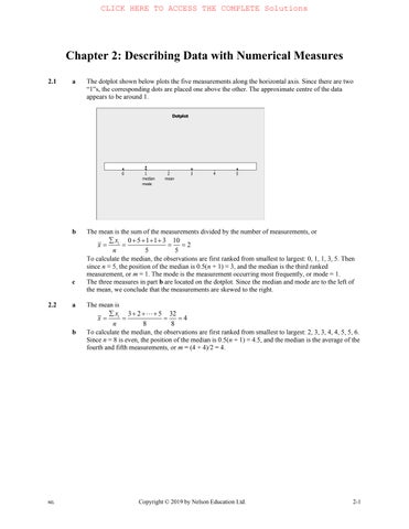
2.1 a The dotplot shown below plots the five measurements along the horizontal axis. Since there are two “1”s, the corresponding dots are placed one above the other. The approximate centre of the data appears to be around 1.
b The mean is the sum of the measurements divided by the number of measurements, or
To calculate the median, the observations are first ranked from smallest to largest: 0, 1, 1, 3, 5. Then since n = 5, the position of the median is 0.5(n + 1) = 3, and the median is the third ranked measurement, or m = 1. The mode is the measurement occurring most frequently, or mode = 1.
c The three measures in part b are located on the dotplot. Since the median and mode are to the left of the mean, we conclude that the measurements are skewed to the right.
2.2 a The mean is
b To calculate the median, the observations are first ranked from smallest to largest: 2, 3, 3, 4, 4, 5, 5, 6. Since n = 8 is even, the position of the median is 0.5(n + 1) = 4.5, and the median is the average of the fourth and fifth measurements, or m = (4 + 4)/2 = 4.
c Since the mean and the median are equal, we conclude that the measurements are symmetric. The dotplot shown below confirms this conclusion.
Dotplot
2.3 a 58 5.8 10 ix x n ===
b The ranked observations are 2, 3, 4, 5, 5, 6, 6, 8, 9, 10. Since 10, n = the median is halfway between the fifth and sixth ordered observations, or m = (5 + 6)/2 = 5.5.
c There are two measurements, 5 and 6, which both occur twice. Since this is the highest frequency of occurrence for the data set, we say that the set is bimodal with modes at 5 and 6.
2.4 a x = å xi n = 52 11 = 4 7
b The ranked observations are 2,2,3,4,5,5,5,6,6,7,7. Since n = 11, the median is halfway at the sixth ordered observation, or m = 5.
c The highest frequency of occurrence for the data set is the measurement 5. The set is unimodal at 5.
2.5 a 10823 1082.3 10 ix
c The average premium cost in different provinces is not as important to the consumer as the average cost for a variety of consumers in his or her geographical area.
2.6 a Although there may be a few households who own more than one DVD player, the majority should own either 0 or 1. The distribution should be slightly skewed to the right.
b Since most households will have only one DVD player, we guess that the mode is 1.
c The mean is
To calculate the median, the observations are first ranked from smallest to largest: There are six 0s, thirteen 1s, four 2s, and two 3s. Then since n = 25, the position of the median is 0.5(n + 1) = 13, which is the thirteenth ranked measurement, or m = 1. The mode is the measurement occurring most frequently, or mode = 1.
d The relative frequency histogram is shown below, with the three measures superimposed. Notice that the mean falls slightly to the right of the median and mode, indicating that the measurements are slightly skewed to the right.
2.7 a The stem and leaf plot below was generated by MINITAB. It is skewed to the right.
Stem and Leaf Plot: Wealth
Stem and leaf of Wealth N = 20
Leaf Unit = 1.0 5 1 78888 (8) 2 00001234 7 2 66 5 3 23 3 3 3 4 3 4 9 2 5 2 1 5 6
b The mean is 536.4 26.82 20 ix x n ===
c Since the mean is strongly affected by outliers, the median would be a better measure of centre for this data set.
2.8 It is obvious that any one family cannot have 2.5 children, since the number of children per family is a quantitative discrete variable. The researcher is referring to the average number of children per family calculated for all families in the United States during the 1930s. The average does not necessarily have to be integer-valued.
2.9 a This is similar to previous exercises. The mean is x = å xi n = 56.5 14 = 4 035
b To calculate the median, rank the observations from smallest to largest. The position of the median is 0.5(n + 1) = 7.5, and the median is the average of the 7th and 8th ranked measurement or m = (4 + 4.25)/2 = 4.125.
c Since the mean is slightly smaller than the median, the distribution is slightly skewed to the left.
2.10 The distribution of sports salaries will be skewed to the right, because of the very high salaries of some sports figures. Hence, the median salary would be a better measure of centre than the mean.
2.11
a This is similar to previous exercises.
2150 215 10 ix x n ===
b The ranked observations are shown below:
175 225 185 230 190 240
190 250 200 265
The position of the median is 0.5(n + 1) = 5.5 and the median is the average of the fifth and sixth observation or 200225 212.5 2 + =
c Since there are no unusually large or small observations to affect the value of the mean, we would probably report the mean or average time on task.
2.12 a This is similar to previous exercises. 417 23.17 18 ix x n ===
The ranked observations are shown below: 4 6 7
The median is the average of the 9th and 10th observations or m = (20 + 20)/2 = 20 and the mode is the most frequently occurring observation mode = 19, 20, 40.
b Since the mean is larger than the median, the data are skewed to the right.
c The dotplot is shown below. Yes, the distribution is skewed to the right.
2.13 a x = å xi n = 16679 82 10 = 1667.98
b The ranked data are 499.99, 599.95, 649.99, 999.99, 1299.99, 1349.99, 1429.99, 1599.99, 1749.99, 6499.99, and the median is the average of the fifth and sixth observations or
m = 1299 99 +1349 99 2 = 1324.99
c Average cost would not be as important as many other variables, such as picture quality, sound quality, size, lowest cost for the best quality, and many other considerations.
2.14 a The sample mean is 863...810 6.412 17 +++++ == x
b We arrange the data in increasing order: {0,1,2,2,3,4,5,5,6,6,7,8,8,8,10,11,23}. The median is the number in the 0.5(n + 1) = 9th position, which is 6. The mode is the number that occurs most often, which in this case is 8.
c Since the mean and median are only slightly off from each other, there is only slight skewness.
d The use of the median is probably better than the mean in this case, as the point with value 23 is likely an outlier (and the median is less sensitive to outliers). The mode is rarely employed in practice.
2.15 a The sample mean is x = å xi n = 62 53 10 = 6.253.
b No, mode is used for large data sets and does not contribute any meaning to this exercise. No, median does not provide any meaningful information. The median only shows if the distribution is centred at the mean
c The plot of time against years is below for Rich Eisen’s 40-yard dash time for the past 10 years.
The biggest improvement is from 2005 to 2006.
d It seems that the 40-yard dash time will decrease in 2015 by the trend of the plot of time against years. It is difficult to say by how much the time will decrease since there is no real pattern of decrease in the plot. 2.16 a 12 2.4 5 ix x
b Create a table of differences, ( ) i xx and their squares, ( )2 i xx
c The sample standard deviation is the positive square root of the variance or 2 2.81.673 ss===
d Calculate 222221540. ix =+++= Then ( ) ( ) 22 2 2 12 4011.252.8 144 i i x x n s n −− ==== and 2 2.81.673 ss=== The results of parts b and c are identical.
2.17 a The range is R = 4 − 1 = 3.
b 17 2.125 8 ix x n ===
c Calculate
Then
2.18 a The range is 615. R =−=
b 31 3.875 8 ix x n ===
c Calculate 2222315137. ix =+++= Then ( ) ( ) 22 2 2 31 13716.87582.4107 177 i i x x n s n −− ==== and 2 2.41071.55 ss===
d The range, R = 5, is 51.553.23 = standard deviations.
2.19 a x = å xi n = 31 6 = 5 17
b The range is R = 9 - 2 = 7
c Calculate å xi 2 = 62 + 72 + 32 + 42 + 22 + 92 = 195 Then s 2 = å xi 2å xi ( )2 n n -1 = 195961( )2 6 5 = 34 833 5 = 6.97 and s = s 2 = 6.97 = 2.64
2.20 a The range is R = 2.39 − 1.28 = 1.11.
b Calculate 22221.282.391.5115.415. ix =+++= Then
c The range, R = 1.11, is 1.11.4362.5 = standard deviations.
2.21 a The range is R = 300 32 – 180.36 = 119.96
b x = å xi n = 3010.19 12 = 250.85
c Calculate Then s 2 =
2.22 a The range of the data is R = 6 − 1 = 5 and the range approximation with n = 10 is 1.67. 3 R s =
b The standard deviation of the sample is
which is very close to the estimate for part a.
c–e From the dotplot below, you can see that the data set is not mound-shaped. Hence, you can use Tchebysheff’s Theorem, but not the Empirical Rule, to describe the data.
2.23 a First calculate the intervals: 363or33 to 39
2366or30to 42
3369or27to 45 xs
According to the Empirical Rule, approximately 68% of the measurements will fall in the interval 33 to 39; approximately 95% of the measurements will fall between 30 and 42; approximately 99.7% of the measurements will fall between 27 and 45.
b If no prior information as to the shape of the distribution is available, we use Tchebysheff’s Theorem. We would expect at least ( ) 2 1110 −= of the measurements to fall in the interval 33 to 39; at least
( ) 2 11234 −= of the measurements to fall in the interval 30 to 42; at least ( ) 2 11389 −= of the measurements to fall in the interval 27 to 45.
2.24 a The interval from 40 to 60 represents 5010.= Since the distribution is relatively moundshaped, the proportion of measurements between 40 and 60 is 68% according to the Empirical Rule and is shown below.
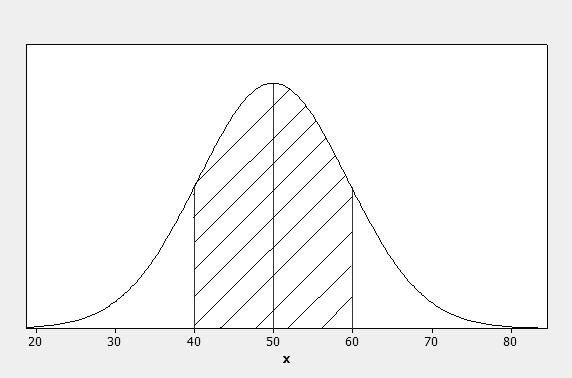
b Again, using the Empirical Rule, the interval 2502(10)= or between 30 and 70 contains approximately 95% of the measurements.
c Refer to the figure below.
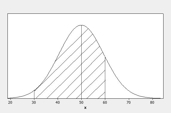
Since approximately 68% of the measurements are between 40 and 60, the symmetry of the distribution implies that 34% of the measurements are between 50 and 60. Similarly, since 95% of the measurements are between 30 and 70, approximately 47.5% are between 30 and 50. Thus, the proportion of measurements between 30 and 60 is 0.34 + 0.475 = 0.815.
d From the figure in part a, the proportion of the measurements between 50 and 60 is 0.34 and the proportion of the measurements which are greater than 50 is 0.50. Therefore, the proportion that are greater than 60 must be 0.5 − 0.34 = 0.16.
2.25 Since nothing is known about the shape of the data distribution, you must use Tchebysheff’s Theorem to describe the data.
a The interval from 60 to 90 represents 3 which will contain at least 8/9 of the measurements.
b The interval from 65 to 85 represents 2 which will contain at least 3/4 of the measurements.
c The value x = 65 lies two standard deviations below the mean. Since at least 3/4 of the measurements are within two standard deviation range, at most 1/4 can lie outside this range, which means that at most 1/4 can be less than 65.
2.26 a The range of the data is R = 1.1− 0.5 = 0.6 and the approximate value of s is 0.2. 3 R s =
b Calculate 7.6 ix = and 2 6.02, ix = the sample mean is 7.6 .76 10 0 ix x n === and the standard deviation of the sample is
22
which is very close to the estimate from part a
2.27 a The stem and leaf plot generated by MINITAB shows that the data is roughly mound-shaped. Note, however, the gap in the centre of the distribution and the two measurements in the upper tail.
Stem and Leaf Plot: Weight Stem and leaf of Weight N = 27 Leaf Unit = 0.010
b Calculate 28.41 ix =
c The following table gives the actual percentage of measurements falling in the intervals xks for 1,2,3. k
d The percentages in part c do not agree too closely with those given by the Empirical Rule, especially in the 1 standard deviation range. This is caused by the lack of mounding (indicated by the gap) in the centre of the distribution.
e The lack of any 1-kilogram packages is probably a marketing technique intentionally used by the supermarket. People who buy slightly less than 1-kilogram would be drawn by the slightly lower price, while those who need exactly 1-kilogram of meat for their recipe might tend to opt for the larger package, increasing the store’s profit.
2.28 According to the Empirical Rule, if a distribution of measurements is approximately mound-shaped, a approximately 68% or 0.68 of the measurements fall in the interval 122.3 or 9.7 to 14.3 = b approximately 95% or 0.95 of the measurements fall in the interval 2124.6or 7.4 to 16.6 =
c approximately 99.7% or 0.997 of the measurements fall in the interval 3126.9or 5.1 to 18.9
=
Therefore, approximately 0.3% or 0.003 will fall outside this interval.
2.29 a The stem and leaf plots are shown below. The second set has a slightly higher location and spread.
Stem and Leaf Plot: Method 1, Method 2
Stem and leaf of Method 1 N = 10
Leaf Unit = 0.00010
Stem-and-leaf of Method 2 N = 10
Leaf Unit = 0.00010 1 10 0 3 11 00
b Method 1: Calculate 0.125 ix = and 2 0.001583 ix = . Then 0.0125 i
Method 2: Calculate
and
The results confirm the conclusions of part a
2.30 a The centre of the distribution should be approximately halfway between 0 and 9 or ( ) 0924.5. +=
b The range of the data is R = 9 − 0 = 9. Using the range approximation, 4942.25. sR==
c Using the data entry method the students should find 4.586 x = and 2.892, s = which are fairly close to our approximations.
2.31 a Similar to previous exercises. The intervals, counts, and percentages are shown in the table.
b The percentages in part a do not agree with those given by the Empirical Rule. This is because the shape of the distribution is not mound-shaped, but flat.
2.32 a Although most of the animals will die at around 32 days, there may be a few animals that survive a very long time, even with the infection. The distribution will probably be skewed right.
b Using Tchebysheff’s Theorem, at least 3/4 of the measurements should be in the interval 3272 or 0 to 104 days.
2.33 a The value of x is 32364.−=−=−
b The interval is 3236 should contain approximately ( ) 1006834% −= of the survival times, of which 17% will be longer than 68 days and 17% less than –4 days.
c–d The latter is clearly impossible. Therefore, the approximate values given by the Empirical Rule are not accurate, indicating that the distribution cannot be mound-shaped.
2.34 a We choose to use 12 classes of length 1.0. The tally and the relative frequency histogram follow.
The three intervals, xks for 1,2,3 k = are calculated below. The table shows the actual percentage of measurements falling in a particular interval as well as the percentage predicted by Tchebysheff’s Theorem and the Empirical Rule. Note that the Empirical Rule should be fairly accurate, as indicated by the mound-shape of the histogram in part a
2.35 a Calculate R = 6 – 1.75 = 4.25, so that s » R 4 = 4.25 4 = 1.0625
b Calculate n = 14, å xi = 56.5, and å xi 2 = 3192.25. Then
and s = 1 826 = 1 351 which is fairly close to the approximate value of s from part a
2.36 a–b Calculate R = 93− 51 = 42, so that 442410.5. sR==
c Calculate 30,2145, inx== and 2 158,345. ix = Then ( ) ( ) 22
and 171.637913.101 s == which is fairly close to the approximate value of s from part b.
d The two intervals are calculated below. The proportions agree with Tchebysheff’s Theorem, but are not to close to the percentages given by the Empirical Rule. (This is because the distribution is not quite mound-shaped.)
2.37 a The number of users who tweeted close to the average number of tweets per user (6.59) is very small in comparison to the number of users who tweeted very little (1,2,3 tweets) or a lot (10 tweets). In other words, the data is spread out. This means that the variance and standard deviation will be large.
b Initially, there is very little variance in the average number of tweets depending on the number of followers and followees. The variance in the average number of tweets as a function of followees starts to increase significantly after about 500 followees. Similarly, the variance for the average number of tweets as a function of followers starts to increase significantly at approximately 300 followers. Here, for some followers the average number of tweets is very small, but for many others the average number of tweets is large, reaching between 100 and 1000. As the average number of followers and followees increases further, so will the variance of the average number of tweets.
2.38 a Answers will vary. A typical stem and leaf plot is generated by MINITAB.
Stem and Leaf Plot: Goals
Stem and leaf of Goals N = 21 Leaf Unit = 1.0
b Calculate 21,940, inx== and 2 53,036. ix = Then 940 44.76, 21 i
c Calculate 244.7646.82or 2.06to91.58. xs
From the original data set, 20 of the measurements, or 95.24% fall in this interval.
2.39 a The sample standard deviation is
b The range is the largest minus the smallest value: 1.329 – 1.104 = 0.225. The range is about three times as big as the standard deviation. Both the range and the standard deviation measure the amount of “spread” in the data.
c The approximation for s based on R (as given in Section 2.5 of the text) is s » R 4 = 0 225 4 = 0.0563 in this case. The approximation is not very accurate.
d After subtracting 0.5, the sample variance is re-computed and turns out to be
9 8 = 00656
Sample variance from part a is 0.0656 (by squaring s computed in part a). Thus, subtracting (or adding) 0.5 (or any constant) does affect the sample variance.
e For this example, three standard deviations from the mean is 1.2339 ± 3(0.0810) = (0.99, 1.48). As can be seen, 100% of the data lies in this interval, which is consistent with Tchebysheff’s Theorem (which predicts that at least 2 1 188.89% 3 −=
of the data/points are within 3 standard deviations from the position of the mean).
f For one standard deviation from the mean, the interval is 1.2339 ± 1(0.0810) = (1.15, 1.31), which contains roughly 6 out of the 9 points, or 66.67%. For 2 standard deviations from the mean, the interval is 1.2339 ± 2(0.0810) = (1.07, 1.40), which contains 9 out of the 9 points, or 100%. The Empirical Rule states that roughly 68% of the data is within 1 standard deviation, and 95% is within 2 standard deviations of the mean. Our results are fairly close (for such a small data set), indicating that our data might be mound-shaped.
g Cannot tell without more information.
2.40 a Calculate
b Using the frequency table and the grouped formulas, calculate 0(4)1(5)2(2)3(4)21 iixf =+++= 22222
2.41 Use the formulas for grouped data given in Exercise 2.40. Calculate 17,79, iinxf== and 2 393. iixf = Then,
2.42 a The data in this exercise have been arranged in a frequency table.
Using the frequency table and the grouped formulas, calculate 0(10)1(5)10(1)46 iixf =+++= 22220(10)1(5)10(1)268 iixf =+++= Then
b–c The three intervals xks for 1,2,3 k = are calculated in the table along with the actual proportion of measurements falling in the intervals. Tchebysheff’s Theorem is satisfied and the approximation given by the Empirical Rule are fairly close for 2 k = and 3. k =
2.43 The ordered data are 0, 1, 3, 4, 4, 5, 6, 6, 7, 7, 8.
a With n = 12, the median is in position 0.5(1)6.5, n += or halfway between the sixth and seventh observations. The lower quartile is in position 0.25(1)3.25 n += (one-fourth of the way between the third and fourth observations) and the upper quartile is in position 0.75(1)9.75 n += (three-fourths of the way between the ninth and tenth observations). Hence, ( ) 1 5625.5,30.25(43)3.25mQ=+==+−= and 3 60.75(76)6.75. Q =+−= Then the five-number summary is
and 31 6.753.253.50 IQRQQ=−=−=
b Calculate 12,57, inx== and 2 337. ix = Then 57 4.75 12 ix x n === and the sample standard deviation is ( )
c For the smaller observation, x = 0, 04.75 1.94 2.454 -score xx z s =− == and for the largest observation, x = 8, 84.75 1.32 2.454 -score xx z s = == Since neither z-score exceeds 2 in absolute value, none of the observations are unusually small or large.
2.44 The ordered data are 0, 1, 5, 6, 7, 8, 9, 10, 12, 12, 13, 14, 16, 19, 19. With n = 15, the median is in position 0.5(1)8, n += , so that m = 10. The lower quartile is in position 0.25(1)4 n += so that 1 6 Q = and the upper quartile is in position 0.75(1)12 n += so that 3 14. Q = Then the five-number summary is
Min Q1 Median Q3 Max 0 6 10 14 19 and 31 1468. IQRQQ=−=−=
2.45 The ordered data are 12, 18, 22, 23, 24, 25, 25, 26, 26, 27, 28.
For n = 11, the position of the median is 0.5(1)0.5(111)6 n +=+= and m = 25. The positions of the quartiles are 0.25(1)3 n += and 0.75(1)9, n += so that 1322,26,QQ== and 26224. IQR =−=
The lower and upper fences are:
The only observation falling outside the fences is x = 12, which is identified as an outlier. The box plot is shown below. The lower whisker connects the box to the smallest value that is not an outlier, x = 18. The upper whisker connects the box to the largest value that is not an outlier or x = 28.
2.46 The ordered data are 2, 3, 4, 5, 6, 6, 6, 7, 8, 9, 9, 10, 22.
For n = 13, the position of the median is 0.5(1)0.5(131)7 n +=+= and m =6. The positions of the quartiles are 0.25(1)3.5 n += and 0.75(1)10.5, n += so that 134.5,9,QQ== and 94.54.5. IQR =−=
The lower and upper fences are: 1 3 1.54.56.752.25
The value x = 22 lies outside the upper fence and is an outlier. The box plot is shown below. The lower whisker connects the box to the smallest value that is not an outlier, which happens to be the minimum value, x = 2. The upper whisker connects the box to the largest value that is not an outlier or x = 10.
2.47 The ordered data are 3, 6, 15, 21, 25, 32, 36, 42, 44, 181.
For n = 10, the position of the median is 0.5(1)0.5(101)5.5 n +=+= and m = (25+32)/2 = 28.5. The positions of the quartiles are 0.25(1)2.75 n += and 0.75(1)8.25, n += so that 1312.75,42.5,QQ== and 42.512.7529.75. IQR =−=
The lower and upper fences are:
QIQR
The value x = 181 lies outside the upper fence and is an outlier. The box plot is shown below. The lower whisker connects the box to the smallest value that is not an outlier, which happens to be the minimum value, x = 3. The upper whisker connects the box to the largest value that is not an outlier, or x = 44.
2.48 From Section 2.6, the 69th percentile implies that 69% of all students scored below your score, and only 31% scored higher.
2.49 a The ordered data are shown below:
For n = 28, the position of the median is0.5(1)14.5 n += and the positions of the quartiles are 0.25(1)7.25 n += and 0.75(1)21.75. n += The lower quartile is one-fourth the way between the seventh and eighth measurements or 1 1180.25(168118)130.5 Q =+−= and the upper quartile is three-fourths the way between the 21st and 22nd measurements or 3 3160.75(318316)317.5. Q =+−= Then the five-number summary is
b Calculate 31 317.5130.5187. IQRQQ=−=−= Then the lower and upper fences are 1 3 1.5130.5280.5150
The box plot is shown below. Since there are no outliers, the whiskers connect the box to the minimum and maximum values in the ordered set.
c–d The box plot does not identify any of the measurements as outliers, mainly because the large variation in the measurements cause the IQR to be large. However, students should notice the extreme difference in the magnitude of the first four observations taken on young dolphins. These animals have not been alive long enough to accumulate a large amount of mercury in their bodies.
2.50 a See Exercise 2.27b.
b For x = 1.38, 1.381.05 -score1.94 0.17 xx z s === while for x = 1.41, 1.411.05 -score2.12 0.17 xx z s ===
The value x = 1.41 would be considered somewhat unusual, since its z-score exceeds 2 in absolute value.
c For n = 27, the position of the median is0.5(1)0.5(271)14 n +=+= and m = 1.06. The positions of the quartiles are 0.25(1)7 n += and 0.75(1)21, n += so that 130.92,1.17,QQ== and 1.170.920.25. IQR =−=
The lower and upper fences are:
The box plot is shown below. Since there are no outliers, the whiskers connect the box to the minimum and maximum values in the ordered set.
Since the median line is almost in the centre of the box, the whiskers are nearly the same lengths, and the data set is relatively symmetric.
2.51 a For n = 15, the position of the median is 0.5(1)8 n += and the positions of the quartiles are 0.25(1)4 n += and 0.75(1)12. n += The sorted measurements are shown below.
Lemieux: 1, 6, 7, 17, 19, 28, 35, 44, 45, 50, 54, 69, 69, 70, 85 Hull: 0, 1, 25, 29, 30, 32, 37, 39, 41, 42, 54, 57, 70, 72, 86
For Mario Lemieux, 13 44,17,69mQQ=== For Brett Hull, 13 39,29,57mQQ===
Then the five-number summaries are
b For Mario Lemieux, calculate 31 691752. IQRQQ=−=−= Then the lower and upper fences are: 1 3 1.5177861 1.56978147 QIQR QIQR −=−=−
For Brett Hull, 31 572928. IQRQQ=−=−= Then the lower and upper fences are:
There are no outliers, and the box plots are shown below.
c Answers will vary. The Lemieux distribution is roughly symmetric, while the Hull distribution seems little skewed. The Lemieux distribution is slightly more variable; it has a higher IQR and a higher median number of goals scored.
2.52 The distribution is fairly symmetric with two outliers (24th and 33rd general elections).
2.53 a Just by scanning through the 26 measurements, it seems that there are a few unusually large measurements, which would indicate a distribution that is skewed to the right.
b The position of the median is 0.5(1)0.5(261)13.5 n +=+= and m = 108697.5. The mean is 3152448 121248 26 ix x n === which is larger than the median, indicating a distribution skewed to the right.
c The positions of the quartiles are 0.25(1)6.75 n += and 0.75(1)20.25 n += so that 1378792,146341.8,QQ== and 146341.757879267549.75. IQR =−= The lower and upper fences are: 1 3 1.5787921.5(67549.75)22532.625 1.5146341.81.5(67549.75)247666.375
The box plot is shown below Since there are no outliers, the whiskers connect the box to the minimum and maximum values in the ordered set. Since the median line is almost in the centre of the box, the whiskers are nearly the same lengths, and the data set is relatively symmetric.
2.54 a The sorted data is 154.54, 175.67, 184.69, 195.65, 198.65, 215.12, 231.91, 254.32, 255.76, 267.34, 267.75, 289.82.
The positions of the median and the quartiles are 0.5(1)6.5, n += 0.25(1)3.25 n += and 0.75(1)9.75, n += so that m = (215.12 + 231.91)/2 = 223.52, 1 184.698.22192.91 Q =+= , 3 255.762.895258.66 Q =+= , and 258.66192.91 IQR =−
QIQR
The lower and upper fences are: 1 3 1.5192.911.5(65.75)94.29 1.5258.661.5(65.75)357.29
There are no outliers, and the box plot is shown below.
b Because of the long right whisker, the distribution is slightly skewed to the right.
2.55 Answers will vary. Students should notice the outliers in the female group, that the median female temperature is higher than the median male temperature.
2.56 a The text proposes the following way to find the first quartile: after arranging the data in increasing order, take “the value of x in position 0.25( n + 1) … When 0.25(n + 1) is not an integer, the quartile is found by interpolation, using the values in the two adjacent positions.” For this question, the location is at 0.25(n + 1) = 0.25(14) = 3.5. The average of the third and fourth ordered points is (91.816 + 93.262)/2 = 92.54 = Q1
The text proposes the following way to find the third quartile: after putting the data in increasing order, take “the value of x in position 0.75(n + 1) … When 0.75(n + 1) is not an integer, the quartile is found by interpolation, using the values in the two adjacent positions.” For this question, the location is at 0.75(n + 1) = 0.75(14) = 10.5. The average of the tenth and eleventh ordered points is 115.457 + 117.824)/2 = 116.64 = Q3
b The interquartile range is IQR = Q3 – Q1 = 152.79 – 56.39 = 24.10.
c The text defines the formula for the lower fence as: Q1 – 1.5(IQR) = 92.54 – 1.5(24.10) = 56.39
d The text defines the formula for the upper fence as: Q3 + 1.5(IQR) = 116.34 + 1.5(24.10) = 152.79.
e The box plot is as follows.
f No outliers
g As defined in the text, the z-score is xx z s = For the smallest observation (89.227), the z-score is 89.227104.4816 1.32 11.5398 z ==− For the largest observation (121.273), 121.273104.4816 1.46 11.5398 z == . For the smallest observation, the z-score of −1.32 maybe somewhat unusually small.
h For Hamilton, the z-score is 103.921104.4816 0.05 11.5398 z ==− which is not unusual.
i I would live where it is most expensive, so that people would drive their car less (on average).
2.57 a Calculate 14,367, inx== and 2
b Calculate 14,366, inx== and 2 9644 ix = . Then
and
c The centres are roughly the same; the Sunmaid raisins appear slightly more variable.
2.58 a Calculate the range as R = 15 − 1 = 14. Using the range approximation, 41443.5. sR==
b Calculate 25,155.5, inx== and 2 1260.75. ix = Then
which is very close to the approximation found in part a.
c Calculate 26.226.994xs= or –0.774 to 13.214. From the original data, 24 measurements or ( ) 242510096% = of the measurements fall in this interval. This is close to the percentage given by the Empirical Rule.
2.59 a The largest observation found in the data from Exercise 1.26 is 32.3, while the smallest is 0.2. Therefore, the range is R = 32.3 − 0.2 = 32.1.
b Using the range, the approximate value for s is 432.148.025. sR==
c Calculate 50,418.4, inx== and 2 6384.34. ix = Then ( ) ( ) 22 2 418.4 6384.34 507.671 149 i i x x n s
2.60 a Refer to Exercise 2.59. Since 418.4, ix = the sample mean is 418.4
50 ix x n ===
The three intervals of interest are shown in the following table, along with the number of observations that fall in each interval.
b The percentages falling in the intervals do agree with Tchebysheff’s Theorem. At least 0 fall in the first interval, at least 340.75 = fall in the second interval, and at least 890.89 = fall in the third. The percentages are not too close to the percentages described by the Empirical Rule (68%, 95%, and 99.7%).
c The Empirical Rule may be unsuitable for describing these data. The data distribution does not have a strong mound-shape (see the relative frequency histogram in the solution to Exercise 1.26), but is skewed to the right.
2.61 The ordered data are shown below.
Since n = 50, the position of the median is 0.5(1)25.5 n += and the positions of the lower and upper quartiles are 0.25(1)12.75 n += and 0.75(1)38.25. n += Then ( ) 1 6.16.626.35,2.10.75(2.42.1)2.325,mQ =+==+−= and 3 12.60.25(13.512.6)12.825. Q =+−= Then 12.8252.32510.5. IQR =−=
The lower and upper fences are
QIQR
QIQR −=−=− +=+= and the box plot is shown below. There is one outlier, x = 32.3. The distribution is skewed to the right.
2.62 a For n = 14, the position of the median is 0.5(1)7.5 n += and the positions of the quartiles are 0.25(n + 1) = 3.75 and 0.75(n + 1) = 11.25 The lower quartile is three-fourths the way between the third and fourth measurements or 1 2.50.75(0.75)3.06 Q =+= and the upper quartile is onefourth the way between the eleventh and twelfth measurements or 3 5.250.25(0.25)5.31 Q =+= Then the five-number summary is
b Calculate 31 5.313.062.25 IQRQQ=−=−= Then the lower and upper fences are 1 3 1.53.061.5(2.25)0.32 1.55.311.5(2.25)8.685
QIQR QIQR −=−=− +=+=
The box plot is shown below. Since there are no outliers, the whiskers connect the box to the minimum and maximum values in the ordered set.
c Calculate
The z-score for x = 1.92 is
2.63 First calculate the intervals:
, which is somewhat unlikely.
0.170.01 xs= or 0.16 to 0.18
20.170.02xs= or 0.15 to 0.19
30.170.03xs= or 0.14 to 0.20
a If no prior information as to the shape of the distribution is available, we use Tchebysheff’s Theorem. We would expect at least ( ) 2 1110 −= of the measurements to fall in the interval 0.16 to 0.18; at least ( ) 2 11234 −= of the measurements to fall in the interval 0.15 to 0.19; and at least ( ) 2 11389 −= of the measurements to fall in the interval 0.14 to 0.20.
b According to the Empirical Rule, approximately 68% of the measurements will fall in the interval 0.16 to 0.18; approximately 95% of the measurements will fall between 0.15 to 0.19; and approximately 99.7% of the measurements will fall between 0.14 and 0.20. Since mound-shaped distributions are so frequent, if we do have a sample size of 30 or greater, we expect the sample distribution to be mound-shaped. Therefore, in this exercise, we would expect the Empirical Rule to be suitable for describing the set of data.
c If the chemist had used a sample size of four for this experiment, the distribution would not be mound-shaped. Any possible histogram we could construct would be non-mound-shaped. We can use at most four classes, each with frequency 1, and we will not obtain a histogram that is even close to mound-shaped. Therefore, the Empirical Rule would not be suitable for describing n = 4 measurements.
2.64 Since it is not obvious that the distribution of amount of chloroform per litre of water in various water sources is mound-shaped, we cannot make this assumption. Tchebysheff’s Theorem can be used, however, and the necessary intervals and fractions falling in these intervals are given in the table.
k xks Interval Tchebysheff
1 3453 –19 to 87 at least 0
2 34106 –72 to 140 at least 0.75
3 34159 –125 to 193 at least 0.89
2.65 The following information is available:
2 400,600,4900nxs ===
The standard deviation of these scores is then 70, and the results of Tchebysheff’s Theorem follow:
k xks Interval Tchebysheff
1 60070 530 to 670 at least 0
2 600140 460 to 740 at least 0.75
3 600210 390 to 810 at least 0.89
If the distribution of scores is mound-shaped, we use the Empirical Rule, and conclude that approximately 68% of the scores would lie in the interval 530 to 670 (which is xs ). Approximately 95% of the scores would lie in the interval 460 to 740.
2.66 a Calculate 10,68.5 inx== , 2 478.375. ix = Then
b The z-score for x = 8.5 is 8.56.85 1.64 1.008 xx z s ===
This is not an unusually large measurement.
c The most frequently recorded measurement is the mode or x = 7 hours of sleep.
d For n = 10, the position of the median is 0.5(1)5.5 n += and the positions of the quartiles are 0.25(1)2.75 n += and 0.75(1)8.25. n += The sorted data are 5, 6, 6, 6.75, 7, 7, 7, 7.25, 8, 8.5. Then ( ) 1 7727,60.75(66)6mQ=+==+−= and 3 7.250.25(87.25)7.4375. Q =+−= Then 7.437561.4375 IQR =−= and the lower and upper fences are 1 3 1.562.156253.84 1.57.43752.156259.59
QIQR −=−= +=+=
There are no outliers (confirming the results of part b) and the box plot is shown below
2.67 a Answers will vary. A typical histogram is shown below. The distribution is slightly skewed to the left.
b Calculate
c The sorted data is shown below:
The z-scores for x = 7.9 and x = 11.3 are
Since neither of the z-scores are greater than 3 in absolute value, the measurements are not judged to be outliers.
d The position of the median is 0.5(1)10.5 n += and the median is m = (9.7 + 9.8)/2 = 9.75.
e The positions of the quartiles are 0.25(1)5.25 n += and 0.75(1)15.75. n += Then 1 9.40.25(9.49.4)9.4 Q =+−= and 3 10.00.75(10.110.0)10.075. Q =+−=
2.68 Refer to Exercise 2.67. Calculate 10.0759.40.675. IQR =−= The lower and upper fences are 1 3 1.59.41.5(.675)8.3875 1.510.0751.5(.675)11.0875
There are three outliers. The box plot is shown below.
2.69 a The range is R = 71 – 40 = 31 and the range approximation is 43147.75. sR==
b Calculate 10,592, inx== 2 36,014. ix = Then
The sample standard deviation calculated above is of the same order as the approximated value found in part a.
c The ordered set is 40, 49, 52, 54, 59, 61, 67, 69, 70, 71. Since n = 10, the positions of m, Q1, and Q3 are 5.5, 2.75, and 8.25, respectively, and ( ) 5961260, m =+= 1 490.75(5249)51.25, Q =+−= 3 69.25, Q = and 69.2551.2518.0. IQR =−=
The lower and upper fences are 1 3 1.551.2527.0024.25 1.569.2527.0096.25
+=+= and the box plot is shown below. There are no outliers and the data set is slightly skewed left.
2.70 The results of the Empirical Rule follow:
k xks Interval Empirical Rule
1 4205 415 to 425 approximately 0.68
2 42010 410 to 430 approximately 0.95
3 42015 405 to 435 approximately 0.997
Notice that we are assuming that attendance follows a mound-shaped distribution and hence that the Empirical Rule is appropriate.
2.71 If the distribution is mound-shaped with mean , then almost all of the measurements will fall in the interval 3, which is an interval 6 in length. That is, the range of the measurements should be approximately6. In this case, the range is 800 – 200 = 600, so that 6006100. =
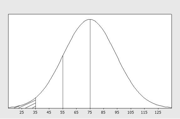
2.72 The stem lengths are approximately normal with mean 38 and standard deviation 5.5. a In order to determine the percentage of roses with length less than 38, we must determine the proportion of the curve which lies within the shaded area (the lower half) in the figure below. Hence, the fraction below 38 would be 50%.
b The proportion of the area between 31 and 51 is 31385138 (3151)(1.272.36)89%
the proportion of the area between 31 and 51 is approximately 89%.
2.73 a The range is R = 172 – 108 = 64 and the range approximation is 464416. sR==
b Calculate 15,2041, inx== 2 281,807. ix = Then 2041
c According to Tchebysheff’s Theorem, with k = 2, at least 3/4 or 75% of the measurements will lie within k = 2 standard deviations of the mean. For this data, the two values, a and b, are calculated as 2136.072(17.10)136.0734.20xs or a = 101.87 and b = 170.27
2.74 The diameters of the trees are approximately mound-shaped with mean 35 and standard deviation 7.
a The value x = 21 lies two standard deviations below the mean, while the value x = 55 is approximately three standard deviations above the mean. Using the Empirical Rule, the fraction of trees with diameters between 21 and 35 is half of 0.95 or 0.475, while the fraction of trees with diameters between 35 and 55 is half of 0.997 or 0.4985. The total fraction of trees with diameters between 21 and 55 is 0.475 + 0.4985 = 0.9735.
b The value x = 43 lies approximately one standard deviation above the mean. Using the Empirical Rule, the fraction of trees with diameters between 35 and 43 is half of 0.68 or 0.34, and the fraction of trees with diameters greater than 43 is approximately 0.5 − 0.34 = 0.16.
2.75
a The range is R = 19 − 4 = 15 and the range approximation is 41543.75. sR==
b Calculate 15,175 inx== , 2 2237. ix = Then 175 11.67 15 i
c Calculate the interval 211.672(3.735)11.677.47xs
or 4.20 to 19.14. Referring to the original data set, the fraction of measurements in this interval is 14/15 = 0.93.
2.76 a It is known that duration times are approximately normal, with mean 75 and standard deviation 20. In order to determine the probability that a commercial lasts less than 35 seconds, we must determine the fraction of the curve that lies within the shaded area in the figure below. Using the Empirical Rule, the fraction of the area between 35 and 75 is half of 0.95 or 0.475. Hence, the fraction below 35 would be 0.5 − 0.475 = 0.025.
b The fraction of the curve area that lies above the 55-second mark may again be determined by using the Empirical Rule. Refer to the figure in part a. The fraction between 55 and 75 is 0.34 and the fraction above 75 is 0.5. Hence, the probability that a commercial lasts longer than 55 seconds is 0.5 + 0.34 = 0.84.
2.77 a The relative frequency histogram for these data is shown below.
b Refer to the formulas given in Exercise 2.40. Using the frequency table and the grouped formulas, calculate
c The three intervals, xks for 2,3 k = are calculated in the table along with the actual proportion of measurements falling in the intervals. Tchebysheff’s Theorem is satisfied and the approximation given by the Empirical Rule are fairly close for 2 k = and 3. k =
2 0.662.78 –2.12 to 3.44 95/100 = 0.95 at least 0.75 0.95
3 0.664.17 –3.51 to 4.83 96/100 = 0.96 at least 0.89 0.997
2.78 a The percentage of universities that have between 145 and 205 professors corresponds to the fraction of measurements expected to lie within two standard deviations of the mean. Tchebysheff’s Theorem states that this fraction will be at least three-fourths or 75%.
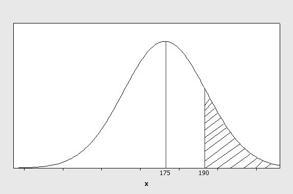
b If the population is normally distributed, the Empirical Rule is appropriate and the desired fraction is calculated. Referring to the normal distribution shown below, the fraction of area lying between 175 and 190 is 0.34, so that the fraction of universities having more than 190 professors is 0.5 − 0.34 = 0.16.
2.79 We must estimate s and compare with the student’s value of 0.263. In this case, n = 20 and the range is R = 17.4 − 16.9 = 0.5. The estimated value for s is then 40.540.125, sR== which is less than 0.263. It is important to consider the magnitude of the difference between the “rule of thumb” and the calculated value. For example, if we were working with a standard deviation of 100, a difference of 0.142 would not be great. However, the student’s calculation is twice as large as the estimated value. Moreover, two standard deviations, or 2(0.263)0.526, = already exceeds the range. Thus, the value s = 0.263 is probably incorrect. The correct value of s is
2.80 Notice that Brett Hull has a relatively symmetric distribution. The whiskers are the same length and the median line is close to the middle of the box. There is an outlier to the right meaning that there is an extremely large number of goals during one of his seasons. The distributions for Mario and Bobby are skewed left, whereas the distribution for Wayne is slightly skewed right. The variability of the distributions is similar for Brett and Bobby. The variability for Mario and Wayne is similar and is much higher than the variability for Brett and Bobby. Wayne has long right whisker, meaning that there may be an unusually
large number of goals during one of his seasons. Mario has the highest IQR and the highest median number of goals. The median number of goals for Brett Hull is the lowest (close to 38); the other three players are all about 41–44.
2.81 a Use the information in the exercise. For 1957 – 80, 21, IQR = and the upper fence is
3 1.5521.5(21)83.5QIQR+=+=
For 1957 – 75, 16, IQR = and the upper fence is
3 1.552.251.5(16)76.25QIQR+=+=
b Although the maximum number of goals in both distribution is the same (77 goals), the upper fence is different in 1957 – 80, so that the record number of goals, x = 77 is no longer an outlier.
2.82 a Calculate 50,418, inx== so that 418 8.36. 50 ix x n ===
b The position of the median is 0.5(n + 1) = 25.5 and m = (4 + 4)/2 = 4.
c Since the mean is larger than the median, the distribution is skewed to the right.
d Since n = 50, the positions of Q1 and Q3 are 0.25(51) = 12.75 and 0.75(51) = 38.25, respectively. Then 1 00.75(10)0.75, Q =+−= 3 170.25(1917)17.5, Q =+−= and 17.50.7516.75. IQR =−=
The lower and upper fences are 1 3 1.5.7525.12524.375 1.517.525.12542.625
and the box plot is shown below. There are no outliers and the data is skewed to the right.
2.83 The variable of interest is the environmental factor in terms of the threat it poses to Canada. Each bulleted statement produces a percentile.
▪ x = toxic chemicals is the 61st percentile.
▪ x = air pollution and smog is the 55th percentile.
▪ x = global warming is the 52nd percentile.
2.84 Answers will vary. Students should notice that the distribution of baseline measurements is relatively mound-shaped. Therefore, the Empirical Rule will provide a very good description of the data. A measurement that is further than two or three standard deviations from the mean would be considered unusual.
2.85 a Calculate 25,104.9 inx== , 2
ix = Then
b The ordered data set is shown below:
c The z-scores for x = 2.5 and x = 5.7 are
Since neither of the z-scores are greater than 3 in absolute value, the measurements are not judged to be unusually large or small.
2.86 a For n = 25, the position of the median is 0.5(1)13 n += and the positions of the quartiles are 0.25(1)6.5 n += and 0.75(1)19.5. n += Then m = 4.2, 1 (3.73.8)/23.75, Q =+= and 3 (4.74.8)/24.75. Q =+= Then the five-number summary is
b–c Calculate 31 4.753.751. IQRQQ=−=−= Then the lower and upper fences are 1 3 1.53.751.52.25 1.54.751.56.25
There are no unusual measurements, and the box plot is shown below.
d Answers will vary. A stem and leaf plot, generated by MINITAB, is shown below. The data is roughly mound-shaped.
Stem and Leaf Plot: Times
Stem and leaf of Times N = 25 Leaf Unit = 0.10


