Kinematics
MULTIPLE CHOICE QUESTIONS
Multiple Choice 2.1
Correct Answer (d). The initial and final position vectors are equal so the difference will be zero. That is, the displacement is zero as calculated from Eq. [2.1]. However, the distance travelled is not zero as this takes into account the path used to travel. Using Eq. [2.2], we see that the average velocity will be zero. However, since the distance is not zero, the average speed will be non-zero and positive.
Multiple Choice 2.2
Correct Answer (d). The accelerations in the xand y-directions are independent, so having the acceleration in one direction being equal to zero does not imply anything specific for the acceleration in the other direction.
Multiple Choice 2.3
Correct Answer (c). As the child moves in a circle, her acceleration is centripetal and, thus, directed toward the centre of curvature. In this case, the centre of curvature is the centre of the circle made by the child and is located where the father stands.
CONCEPTUAL QUESTIONS
Conceptual Question 2.1
Yes, when the object is slowing down.
Conceptual Question 2.2
If the average velocity in a given time interval is zero, the displacement over that time interval must also be zero.
Conceptual Question 2.3
(a) At the moment the object reaches its highest altitude, its velocity is zero and its acceleration is equal to the acceleration due to gravity.
(b) Same as part (a), since the acceleration of the object is constant.
Conceptual Question 2.4
The dog runs at twice the speed of its master for the same amount of time. That means that the dog runs twice as far as its master. Since its master travels a distance of 1.0 km, the dog must travel 2.0 km.
Conceptual Question 2.5
(a) Yes, because the object may change its direction without changing its speed. An example of this is uniform circular motion.
(b) No.
Conceptual Question 2.6
(a) Yes. If the projectile’s velocity has a horizontal component, then, at the top of the trajectory, the velocity is completely horizontal and the gravitational acceleration is vertical.
(b) Along the entire path if the projectile is thrown vertically.
Conceptual Question 2.7
(a) The same as if thrown on steady ground.
(b) The path is the projectile trajectory in the last equation of Case Study 2.2, where v0 , x is the constant horizontal velocity of the train.
Conceptual Question 2.8
Its component along the path of the object accelerates the object; that is, its motion is no longer uniform. The perpendicular component causes a curved path.
Conceptual Question 2.9
(a) Uniform circular motion.
(b) Accelerated motion along a straight line with linear increase (or decrease) in speed.
Conceptual Question 2.10
(a) No; its x- and y-components vary continuously; that is, the velocity in a Cartesian coordinate system is not constant.
(b) Yes; its speed along the path is constant, as no acceleration acts in that direction for a uniform motion.
(c) No. Even though the magnitude of the acceleration is constant, the direction of the acceleration continuously changes.
Conceptual Question 2.11
The gravitational acceleration downward is smaller than the centripetal acceleration required to hold it on a circular path. As a result, the bottom of the bucket has to push the water down when it is at the top of the loop. Newton’s third law then states that the water pushes the bottom of the bucket upward. Compare the water to a person on a fast roller coaster as opposed to a slow Ferris wheel.
ANALYTICAL PROBLEMS
Problem 2.1
(a) We define the vector sum as � r = x , y ( ) so that we can write � r = � a + � b or, in component notation:
x = a x + b x = 5.00 + ( 14.00) = 9.00 y = a y + b y = 5.00 + 5.00 = 10.00.
Thus, � r = (–9.00, 10.00), as shown in Figure 1.
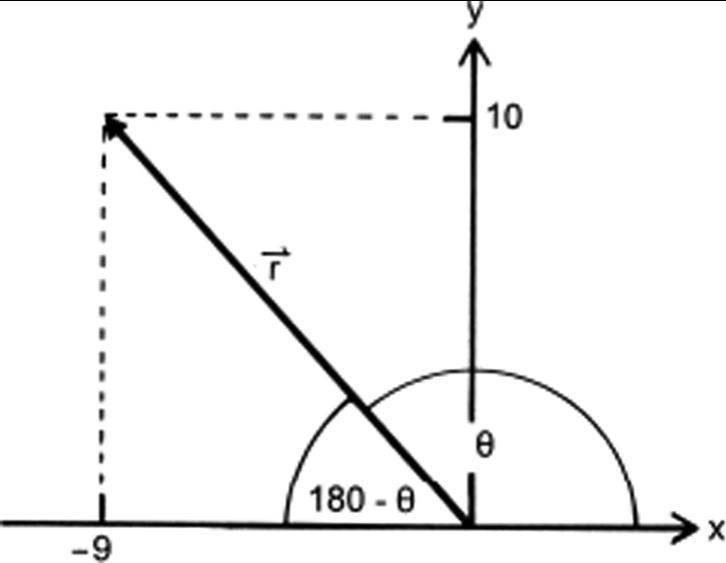
Figure 1
(b) The magnitude of vector � r is calculated with the Pythagorean theorem:
| � r |= x 2 + y 2 = ( 9) 2 + 10 2 = 13.5
To characterize the vector � r in polar coordinates, its angle with the positive x-axis must also be determined. This can be done geometrically, as can be seen from Figure 1: tan θ = y x = 1.11 ⇒ θ = 132°
Problem 2.2
The problem implies two equations, and we write each in component form:
(I) a x + b x = 6.00
(II) a y + b y = 2.00
(III) a x b x = 5.00
(IV) a y b y = 8.00 (1)
Adding the first and third as well as the second and fourth lines of Eq. [1] leads to vector � a :
2 a x = 1.00
2 a y = 10.00
We combine these components to find the magnitude of � a :
� a = 0.52 + 52 = 5.02
Subtracting the third from the first and the fourth from the second lines in Eq. [1] in turn gives � b in component form:
2 b x = 11.00
2 b y = 6.00
and the magnitude of vector � b : � b = 5.52 + ( 3) 2 = 6.2 6.
Problem 2.3
v av = Δx Δt ≈ 27 nm 6.0 s = 4.5 nm s
Problem 2.4
In the (x1, y1)-coordinate system, the red dot is located at coordinates (2, 3), so that the position vector is � r1 = 2, 3 ( ) . In the (x2,y2)-coordinate system, the red dot is located at coordinates ( 2,2), so that the position vector is � r2 = 2, 2 ( )
Note that � r2 = � r1 � a1, where � a1 = ( 4,1) is the position vector for the origin of the (x2,y2)-coordinate system as measured on the (x1,y1)-coordinate system.
Problem 2.5
Using Eq. [2.2], v av = 10.1 m/s = 36.4 km/h.
Problem 2.6
(a) Figure 2 shows the relative position of points A and B in the fracture plane. For convenience, this plane has been chosen as the xy-plane. With this choice of coordinate system, the horizontal slip is along the x-axis, where the point A on the bone has moved to position C . The vertical slip along the vertical y-axis moves the point on the bone from C to point B. To put it another way, point A slips to point B; the horizontal slip is the x-component of the vector AB � and the vertical slip is the ycomponent of AB � . Thus, the displacement from A to B can be written in vector notation:

Figure 2
The total displacement within the fracture plane is 5.0 mm.
(b) Of the two components of displacement considered in part (a) , the horizontal displacement AC � does not contribute to a displacement along the axis of the bone. Fig ure 3 shows how the component of the vertical displacement from part (a) that is , CB � (equivalent to displacement AD � ) relates to the displac ement along the bone’s axis. In Figure 3 , the displacement from point E to point D is the displacement along the bone’s axis (and the displacement from point A to point E is the displacement perpendicular to the bone’s axis).

Figure 3
The angle of q = 20°, given in the problem text, is the angle between the vectors AE � and AD � We can calculate the length of ED � using trigonometry: ED � = AD � sin 20° = ( 3.0 mm ) sin 20° ⇒ ED � = 1.0 mm
The displacement along the bone’s axis is 1.0 mm. In an analogous fashion, it can be shown that the displacement perpendicular to the bone’s axis, that is, the magnitude of the vector given by AE � is 2.8 mm.
Problem 2.7
(a) We choose the origin at the bottom of the feet of the person, with the x-axis pointing horizontal and toward the right and the y-axis pointing straight up. From Figure 2.38, the x-coordinate of the right hand is:
x = d 2sinθ = 80sin35° = 46 cm
The y-coordinate of the right hand is:
y = d1 d 2cosθ
= 150 80cos35° = 85 cm
Therefore:
� d male = 46 ˆ i + 85 ˆ j (1)
(b) Similarly, for the female person:
x = d 2 sin θ
= 65 sin 35° = 37 cm
y = d1 d 2 cos θ
= 130 65 cos 35° = 77 cm.
Therefore, � d female = 37 ˆ i + 77 ˆ j.
Problem 2.8
(a) The distance between the two intersections of the dashed line, with the skull in the top sketch, measures 54 mm. This provides us with a scale for Figure 2.39 because the problem states that the dashed line measures 16 cm for a real skull. That is, to obtain a distance in the real skull, we can multiply the distance measured in the diagram by a factor of 160/54, which is 3.0.
Before analyzing the figure, a coordinate system must be chosen. This is shown in Figure 4, with the direction up chosen to be the z-direction for both sketches, the direction to the observer’s right in the top sketch the x-direction, and the direction toward the back of the skull in the bottom sketch the y-direction.
For convenience, we choose the point A to coincide with the origin of the coordinate system: A = (0, 0, 0). We use the skull in the top sketch to obtain the xand z-coordinates of point B:
x = 1.2 × 3.0 = 3.6 cm,
z = 2.07 × 3.0 = 6.2 cm
Similarly, we can measure the y-coordinate of point B from the bottom diagram in Figure 4:
y = 2.19 × 3.0 = 6.6 cm
Therefore,
AB � = 3.6 cm , 6.6 cm , 6.2 cm ( )
AB � = 3.6 2 + 6.6 2 + 6.2 2 = 9.7 cm


Figure 4
(b) For convenience, we assume that the skull is left–right symmetric, that is, we have only to determine the position of one of the two last maxilla molars. That point coincides with point B in Figure 2.39. Let us define the point between the two central maxilla incisor teeth as point C . Using the same approach as in part (a) and measuring on the top sketch a horizontal distance of 12.5 mm, a vertical distance of 2.0 mm, and, on the bottom sketch, a depth displacement of 20 mm, we find for the
vector CB � = (3.70 cm, 0.60 cm, 5.93 cm). Due to the symmetry, the vector to the other last maxilla molar (called point B’) is CB � ! = (–3.70 cm, 0.60 cm, 5.93 cm). The angle between these two vectors follows from the scalar product:
(3 7, 0 6, 5 93)
( 3 7, 0 6, 5 93) 3 72 + 0 6 2 + 5 932 = 13.69 + 0.36 + 35.16 13 69 + 0 36 + 35 16 = 0.44
Thus, we find φ = 64°. (c) There are two ways to confirm this angle using Figure 2.40. Either you read the angle between the two straight-line segments off the figure directly, using a protractor, or you use a ruler and measure the relevant distances in Figure 5:

Figure 5
The figure shows how the distance between the two last maxilla molars, which is given as BB! � = 2dx, and the distance from that line to point C , dy, are related to the angle q we seek. Measuring the distance between the centres of the two last molars as dx = 42.5 mm and measuring the distance perpendicular as dy = 31.5 mm, we find: tan θ 2 " # $ % & ' = d x d y = 1 2 ( 42.5 mm ) 31.5 mm ) = 0.675
⇒ θ = 68°
This value agrees with φ= 64° within the precision of the analysis. The skull in Figure 2.39 and the top view of the dentition in Figure 2.40 are obtained from
different sources, thus, normal anatomic variations may contribute to the difference of the found values. Note that we did not convert the measurements in part (c) using a scale for Figure 2.39. This is due to the fact that obtaining angles is based on the division of lengths, where such a scale factor cancels anyway.
Problem 2.9
Assume that the bacterium moves along a straight line:
Problem 2.11
We have motion with constant acceleration in both directions. We can write Eq. [2.10] for both the x- and y-directions, using the given initial position, initial velocity, and constant acceleration (all quantities in SI units):
x = 2 3t + t 2 2
y = 3 + 2t + t 2 (1)
Actual bacteria move in random fashion; this type of motion is discussed in Chapter 10.
Problem 2.10
For motion with constant acceleration, the position as a function of time can be found using Eq. [2.10]. With the values of initial position, initial velocity, and constant acceleration, we can write:
= 5 5t 5t 2 , (1)
where we assume all quantities in SI units.

Figure 6
Graphically, Eq. [1] is an inverted parabola, such that, at t = 0 s, the position is x = 5 m and as t increases, x decreases, passing x = 0 m at time t = 0.62 s. At t = 10 s, the position reaches x = 545 m. Qualitatively, the graph is illustrated in Figure 6.

Figure 7
Graphically, both functions in Eq. [1] represent upright parabolas, such that, at t = 0 s, both x and y are positive. However, while the y–t graph is increasing and does not pass by y = 0 m, the graph of x–t is initially decreasing and crosses x = 0 m at t = 0.76 s and later at t = 5.24 s.

Figure 8
Furthermore, x–t is decreasing for time between t = 0 s and t = 3 s and increasing from t = 3 s to t = 10 s. At t = 10 s, the positions are x = 22 m and y = 123 m. In Figure 7, we have the x–t graph while, in Figure 8, we have the y–t graph.
Problem 2.12
(a) The largest speed occurs at point D as it presents the steepest slope.
(b) The smallest non-zero speed occurs at point B, as this is the smallest non-zero slope.
(c) The smallest non-zero velocity occurs at point D , since the slope is negative and, thus, a smaller value than the slope at B.
(d) At points A, C , and E, the velocity is zero, as the position is unchanging at those points.
(e) The object moves to the left at points with negative velocity, that is, point D
Problem 2.13
We will assume that tf = 8 s. Since there are three different accelerations, we split the problem in three parts. From t1 = 0 s to t2 = 2 s, the acceleration is a1 = 2. m/s2. Eq. [2.8] can be used to find the position x2 at t2 = 2 s after accelerating for Δ t = 2 s: x2 = x1 + v1Δt + 1 2 a1Δt 2 = 10 m (1)
We also need the velocity v2 at t2, calculated from Eq. [2.5], after Δ t = 2 s:
v2 = v1 + a1Δt = 1 m s (2)
From t2 = 2 s to t3 = 6 s, we have a2 = 1 m/s2
Eq. [2.8] gives the position x3 at t3 = 6 s, with x2 from Eq. [1] and v2 from Eq. [2], as the object accelerates for Δt = 4 s:
x3 = x2 + v2 Δt + 1 2 a2 Δt 2 = 6 m (3)
We also need the velocity v3 at t3, calculated from Eq. [2.5], after Δ t = 4 s:
v3 = v2 + a2 Δt = 3 m s (4)
In the last segment, from t3 = 6 s to tf = 8 s, we have a3 = 2 m/s2. We use again Eq. [2.8] to find the position xf at tf = 8 s. We use x3 from
Eq. [3] and v3 from Eq. [4] as the object accelerates for Δ t = 2 s:
xf = x3 + v3Δt + 1 2 a3Δt 2 = 4 m
The final x-position of the object is xf = 4 m.
Problem 2.14
The x-direction and y-direction motions are independent of each other, so we can calculate the final x-position and the final y-position separately, using the given information and the accelerations from the graphs. We will assume that tf = 8 s. For the x-direction, since there are three different accelerations, we split the problem in three parts. From t1 = 0 s to t2 = 2 s, the acceleration is a1x = 2 m/s2.
Eq. [2.8] can be used to find the position x2 at t2 = 2 s after accelerating for Δt = 2 s:
x2 = x1 + v1 x Δt + 1 2 a1
(1)
We also need the velocity v2x at t2, calculated from Eq. [2.6], after Δ t = 2 s:
v2 x = v1 x + a1 x Δt = 9 m s (2)
From t2 = 2 s to t3 = 6 s, we have a2x = 1 m/s2. Eq. [2.8] gives the position x3 at t3 = 6 s, with x2 from Eq. [1] and v2x from Eq. [2] as the object accelerates for Δt = 4 s:
46m (3)
We also need the velocity v3x at t3, calculated from Eq. [2.6], after Δ t = 4 s: v3 x = v2 x + a2 x Δt = 5 m s (4)
In the last segment, from t3 = 6 s to tf = 8 s, we have a3x = 2 m/s2. We use again Eq. [2.8] to find the position xf at tf = 8 s. We use x3 from Eq. [3] and v3x from Eq. [4] as the object accelerates for Δ t = 2 s:
xf = x3 + v3 x Δt + 1 2 a3 x Δt 2 = 60 m (5)
For the y-direction, since there are also three different accelerations, we split the problem in three parts. From t1 = 0 s to t2 = 2 s, the acceleration is a1y = 0 m/s2. Eq. [2.42] can be used to find the position y2 at t2 = 2 s after moving for Δ t = 2 s:
y2 = y1 + v1 y Δt = 1m (6)
Since the acceleration is zero, the velocity v2y at t2 is simply:
v2 y = v1 y = 3 m s . (7)
From t2 = 2 s to t3 = 5 s, we have a2y = 1 m/s2. Eq. [2.8] gives the position y3 at t3 = 5 s, with y2 from Eq. [6] and v2y from Eq. [7] as the object accelerates for Δt = 3 s:
y3 = y2 + v2 y Δt + 1 2 a2 y Δt 2 = 5.5 m (8)
We also need the velocity v3y at t3, calculated from Eq. [2.5], after Δ t = 3 s:
v3 y = v2 y + a2 y Δt = 0 m s (9)
In the last segment, from t3 = 5 s to tf = 8 s, we have a3y = 2 m/s2. We use again Eq. [2.8] to find the position yf at tf = 8 s. We use y3 from Eq. [8] and v3y from Eq. [9] as the object accelerates for Δ t = 3 s:
yf = y3 + v3 y Δt + 1 2 a3 y Δt 2 = 14.5m (10)
With the results from Eq. [5] and Eq. [10], we write the final position vector of the object as:
xf , yf ( ) = 60.0 m , 14.5 m ( ) .
Problem 2.15
The average velocity is given by Eq. [2.2]. Although we do not know the initial position
xi, we can find xf in terms of xi and calculate the average velocity:
v av = xf xi Δt (1)
for Δ t = 8 s. The motion is easily divided into five segments: Δt1 = 1 s from t = 0 s to t = 1 s and a1 = 2 m/s2; Δ t2 = 2 s from t = 1 s to t = 3 s and a2 = 0 m/s2; Δ t3 = 2 s from t = 3 s to t = 5 s and a3 = 1 m/s2; Δ t4 = 1 s from t = 5 s to t = 6 s and a4 = 1 m/s2; and the last interval Δt5 = 2 s from t = 6 s to t = 8 s, where a5 = 0 m/s2 From the graph, we also know the initial velocities at each segment are v1 = 0 m/s, v2 = v3 = 2 m/s, v4 = 0, and v5 = 1 m/s. We use Eq. [2.10] in segments 1, 3, and 4 (constant acceleration), and we use Eq. [2.2] in segments 2 and 5 (constant velocity). We find after Δt1:
x1 = xi + 1m. (2)
We use x1 and Δ t2 to find x2: x2 = x1 + 4m = xi + 5m (3)
We use x2 and Δ t3 to find x3:
x3 = x2 + 4 m 2 m = xi + 7 m (4)
We can now use x3 and Δ t4 to find x4:
x4 = x3 + 0 0.5 m = xi + 6.5 m (5)
In the last step, we use x3 and Δ t4 to find:
xf = x4 2 m = xi + 4.5 m (6)
Substituting the value found in Eq. [2] into the average velocity of Eq. [1], we find: v av = 4.5 m 8 s = 0.56 m s .
To find the average speed, we need to calculate the total distance travelled by the object. The object changes direction of motion at t = 5s. Therefore, we need to calculate the displacements from t = 0s to t = 5s and from
t = 5s to t = 8s separately, using the previous method The results are:
Δx05 = 7 m, Δx58 = 2.5 m.
Then, the total distance is d = 7 m + 2.5 m = 9.5 m.
The average speed is now calculated as: speed av = d Δt = 9.5 m 8 s = 1.2 m s
Problem 2.16
You start from rest, with v1 = 0 m/s, and accelerate uniformly at a = 1.00 m/s2 for a distance Δx1 = 15.0 m. We can use Eq. [2.12] to find your maximum speed v2 at the end of the accelerating period:
v2 = v1 2 + 2 aΔx1 = 5.48 m s (1)
Once you reach your maximum speed v2, you move with that constant speed, so we can use Eq. [2.2] to find the total distance Δ x2 you travel from the moment you grab the hat until the moment your friend catches you: Δx2 = Δx1 + v2 Δt 2 = 97 m ,
where Δt2 = 15.0 s is the time you run at your maximum speed v2, given by Eq. [1]. The total time it took your friend to catch you is:
(2)
where Δt1 is the time it took you to accelerate to your maximum speed. We can calculate Δ t1 using Eq. [2.5] and Eq. [1]: Δt1 = v2 v1 a = 5.48 s (3)
Substituting the known value of Δt2 = 15.0 s and Δ t1 from Eq. [3] into Eq. [2], we find the total time to be Δt = 20.5 s.
Problem 2.17
We use Eq. [2.12] with v1 = 0: a = v2 2 v1 2 2 Δx = (11 km s ) 2 2( 220 m ) = 28000 g
Trained humans survive 30g for 1 second, 15g for 5 seconds, 8g for 1 minute, and 6g for less than 4 minutes.
Problem 2.18
The graph is shown in Figure 9.

Figure 9
Problem 2.19
(a) We find ymax using Eq. [2.12] as: ymax = vi 2 2 g = 31.9 m
(b) To reach the highest altitude, it takes a time of t = 2.55 s. This can be calculated using the last equation in Eq. [2.23]
(c) To reach the ground after reaching the highest altitude, it will take the same time as the time to reach the highest altitude, that is, a time of t = 2.55 s.
(d) The object will hit the ground with a speed equal to the initial speed, but directed down, so that vf = –25.0 m/s.
Problem 2.20
We use vi = 0 in Eq. [2.12]:
a = vf 2 2 Δh = (1.0 m s ) 2 2(10.0 m ) = 0.050 m s 2
Problem 2.21
The time it takes for the object to fall from height h when falling from rest can be calculated using Eq. [2.10]:
t = 2 h g (1)
For a height h = 4.0 m, the time from Eq. [1] is, then, t = 0.90 s. If we double the height, the time will increase by a factor of √2 = 1.41. The speed at the instant the object hits the ground can be calculated using Eq. [2.11]:
v = 2 gh (2)
For a height of h = 4.0 m, the speed from Eq. [2] is, then, v = 8.9 m/s. If we increase the height by a factor of four, the speed will increase by a factor of √4 = 2. If the object starts with a non-zero initial speed v0 directed down, we can use Eq. [2.12] to find the final speed as:
v = v0 2 + 2 gh . (3)
For a height of h = 4.0 m, and an initial speed of v0 = 1.0 m/s, Eq. [3] yields v = 8.9 m/s. If, instead, the initial speed is v0 = 2.0 m/s, Eq. [3] yields v = 9.1 m/s. We can conclude that the relationship between initial speed and final speed is clearly not linear, a fact also evident from the expression in Eq. [3].
Problem 2.22
The time tf it takes for the rock to hit the ground can be found using Eq. [2.5]:
t f = v2 v1 a = v2 g = 3.06 s
The initial height h of the rock with respect to the ground can be found with Eq. [2.12]: h = v2 2 2 g = 45.9 m

Figure 10
Figure 10 above shows the acceleration of the rock that is given by: a y t ( ) = g

Figure 11
Figure 11 above shows the velocity of the rock that is given by:
v y t ( ) = gt .

Figure 12
Figure 12 above shows the position of the rock that is given by:
y t ( ) = h 1 2 gt 2
Problem 2.23
The first step is to draw a diagram and set up the coordinate system (see Figure 2.45). The initial velocity of the ball is broken into xand y-components.
We now have all the information needed to use Eqs. [2.23] to solve for (x, y) at time t = 3.00 s:
v x = 10.0 cos 60° = 5.00 m s
x = x0 + v x t = 0 m + (5.00 m s )( 3.0 s ) = 15 m
v0 y = 10.0 sin 60° = 8.66 m s
y = y0 + v0 y t 1 2 gt 2
= 0 m + (8.66 m s )(3.0 s) 1 2 ( 9.8 m s 2 )( 3.0 s ) 2 = 18 m
That means the final position vector of the ball is (15 m, 18 m). This means that, after 3 s, the ball is lower than where it started by 18 m. Perhaps it was thrown off of a 7th floor balcony?
Problem 2.24
(a) The horizontal distance is:
x = v0 cos θ ( ) t
= v0 cos θ ( ) 2 v0 sin θ ( ) g " # $ % & ' = 7.95 m
(b) The maximum height reached in the jump can be calculated as:
ymax = v0 sin θ ( ) t 1 2 g t 2 ,
where the time t needed to reach the maximum height is given by: t = v0 sin θ g .
Substituting the values given in the problem, we find t = 0.38 s and ymax = 0.72 m.
Problem 2.25
The time for the baseball to reach the catcher is:
t = Δx vix = 20.0 m 150 km h = 0.48 s.
During that time, the ball falls a distance of:
y = 1 2 gt 2 = 9.8 m s 2 2 0.48 s ( ) 2 = 1.1 m
Problem 2.26
The time for football to reach the goal is: t = Δx vi cos θ = 3.3 s.
The height at that instant is:
y = vi sin θ ( ) t 1 2 gt 2 = 0.6 m.
Therefore, we can conclude that the ball hits the ground before reaching the goal.
Problem 2.27
(a)
vi = 30 km h 1000 m 1 km ! " # $ % & 1 h 3600 s ! " # $ % & = 8.3 m s
vi,x = vicos45° = 5.9 m s
vi,y = visin45° = 5.9 m s
The time for the fish to reach the highest point (with v1 = 0 in Eq. [2.6]) is:
t = vi,y g = 0.60 s.
The distance travelled during a time of 2t (until re-entry) is:
Δx = vi , x ( 2t ) = 7.1 m
(b) Yes, the fish is definitively gliding.
Problem 2.28
We use Eq. [2.12] in the vertical direction, where, for the elevator starting from rest:
v2 = 6 m s ,
and y2 y1 = 30 m:
Problem 2.29
If the maximum acceleration a pilot may experience during a horizontal circle is seven times the gravitational acceleration, then we are concerned with the pilot’s centripetal acceleration. Therefore, we will find the conditions for the centripetal acceleration to equal 7g and take those conditions as the limits of what the standard man may do. So, our condition for the circular motion is that the acceleration is a⊥ = 7 g . Since the airplane travels at 100 m/s, we can find the radius of the circle using Eq. [2.26]:
a = v 2 r = 7g r = v 2 7g = 100 m s ! " # $ % & 2 7 × 9.8 m s 2 = 146 m
This is the minimum radius of the airplane’s circular path; any smaller and the centripetal acceleration will surpass the given limit. Note that this result is independent of the pilot’s mass.
Problem 2.30
We can find the period first and then use Eq. [2.27] to determine the centripetal acceleration. The period of the ride is given in the information “spins four times per minute.” This means one period takes T = 15 s. Therefore, the centripetal acceleration is:
a = v 2 r = 2πr T " # $ % & ' 2 1 r = 4π 2 r T 2 = 4π 2 9.0 ( ) 152 = 1.6 m s 2